
Abstract
Background
In this research, we explore the application of Convolutional Neural Networks (CNNs) for the development of an automated cancer detection system, particularly for MRI images. By leveraging deep learning and image processing techniques, we aim to build a system that can accurately detect and classify tumors in medical images. The system's performance depends on several stages, including image enhancement, segmentation, data augmentation, feature extraction, and classification. Through these stages, CNNs can be effectively trained to detect tumors in MRI images with high accuracy. This automated cancer detection system can assist healthcare professionals in diagnosing cancer more quickly and accurately, improving patient outcomes. The integration of deep learning and image processing in medical diagnostics has the potential to revolutionize healthcare, making it more efficient and accessible.
Methods
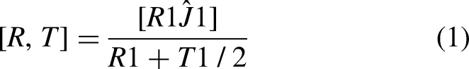
In this paper, we examine the failure of semantic segmentation by predicting the mean intersection over union (mIoU), which is a standard evaluation metric for segmentation tasks. mIoU calculates the overlap between the predicted segmentation map and the ground truth segmentation map, offering a way to evaluate the model's performance. A low mIoU indicates poor segmentation, suggesting that the model has failed to accurately classify parts of the image. To further improve the robustness of the system, we introduce a deep neural network capable of predicting the mIoU of a segmentation map. The key innovation here is the ability to predict the mIoU without needing access to ground truth data during testing. This allows the system to estimate how well the model is performing on a given image and detect potential failure cases early in the process. The proposed method not only predicts the mIoU but also uses the expected mIoU value to detect failure events. For instance, if the predicted mIoU falls below a certain threshold, the system can flag this as a potential failure, prompting further investigation or triggering a safety mechanism in the autonomous vehicle. This mechanism can prevent the vehicle from making decisions based on faulty segmentation, improving safety and performance. Furthermore, the system is designed to handle imbalanced data, which is a common challenge in training deep learning models. In autonomous driving, certain objects, such as pedestrians or cyclists, might appear much less frequently than other objects like vehicles or roads. The imbalance can cause the model to be biased toward the more frequent objects. By leveraging the expected mIoU, the method can effectively balance the influence of different object classes, ensuring that the model does not overlook critical elements in the scene. This approach offers a novel way of not only training the model to be more accurate but also incorporating failure prediction as an additional layer of safety. It is a significant step forward in ensuring that autonomous systems, especially self-driving cars, operate in a safe and reliable manner, minimizing the risk of accidents caused by misinterpretations of visual data. In summary, this research introduces a deep learning model that predicts segmentation performance and detects failure events by using the mIoU metric. By improving both the accuracy of semantic segmentation and the detection of failures, we contribute to the development of more reliable autonomous driving systems. Moreover, the technique can be extended to other domains where segmentation plays a critical role, such as medical imaging or robotics, enhancing their ability to function safely and effectively in complex environments.
Results and Discussion
Brain tumor detection from MRI images is a critical task in medical image analysis that can significantly impact patient outcomes. By leveraging a hybrid approach that combines traditional image processing techniques with modern deep learning methods, this research aims to create an automated system that can segment and identify brain tumors with high accuracy and efficiency. Deep learning techniques, particularly CNNs, have proven to be highly effective in medical image analysis due to their ability to learn complex features from raw image data. The use of deep learning for automated brain tumor segmentation provides several benefits, including faster processing times, higher accuracy, and more consistent results compared to traditional manual methods. As a result, this research not only contributes to the development of advanced methods for brain tumor detection but also demonstrates the potential of deep learning in revolutionizing medical image analysis and assisting healthcare professionals in diagnosing and treating brain tumors more effectively.
Conclusion
In conclusion, this research demonstrates the potential of deep learning techniques, particularly CNNs, in automating the process of brain tumor detection from MRI images. By combining traditional image processing methods with deep learning, we have developed an automated system that can quickly and accurately segment tumors from MRI scans. This system has the potential to assist healthcare professionals in diagnosing and treating brain tumors more efficiently, ultimately improving patient outcomes. As deep learning continues to evolve, we expect these systems to become even more accurate, robust, and widely applicable in clinical settings. The use of deep learning for brain tumor detection represents a significant step forward in medical image analysis, and its integration into clinical workflows could greatly enhance the speed and accuracy of diagnosis, ultimately saving lives. The suggested plan also includes a convolutional neural network-based classification technique to improve accuracy and save computation time. Additionally, the categorization findings manifest as images depicting either a healthy brain or one that is cancerous. CNN, a form of deep learning, employs a number of feed-forward layers. Additionally, it functions using Python. The Image Net database groups the images. The database has already undergone training and preparation. Therefore, we have completed the final training layer. Along with depth, width, and height feature information, CNN also extracts raw pixel values.We then use the Gradient decent-based loss function to achieve a high degree of precision. We can determine the training accuracy, validation accuracy, and validation loss separately. 98.5% of the training is accurate. Similarly, both validation accuracy and validation loss are high.
Introduction
One of the most challenging problems in medical image processing is picture segmentation.Brain tumour segmentation is a novel approach in this area.This study focuses on the current changes in deep learning techniques in this subject. Firstly, we provide a brief overview of brain tumours and their classification. We then discuss these latter algorithms, highlighting the current advancements in deep learning techniques. Lastly, we provide an evaluation of the current state of affairs and discuss proposals for standardizing MRI-based techniques for brain cancer classification. Brain cancer is a rare and fatal illness that offers minimal chances of recovery. One of neurologists’ and radiologists’ most crucial tasks is the early diagnosis of brain tumors. Recent claims suggest that computer-aided diagnostic systems, using magnetic resonance imaging (MRI) as a supporting technology, can detect brain tumours. In this work, we suggest transfer learning techniques for a deep learning model that can identify malignant tumors, such as glioblastoma, using MRI data. This study demonstrates the use of deep learning in conjunction with the state-of-the-art object detection framework, YOLO (You Only Look Once), to detect and categorize brain tumors. A novel deep learning technique for identifying items that need less processing power than its rivals is called YOLOv5. The research made use of the Brats 2021 dataset from the RSNA-MICCAI brain tumour radio genomic classification. We used the make sense AI online labelling tool to label images from the RSNA-MICCAI brain tumour radio genomic competition dataset. Next, we divide the previously processed data into two groups: training and testing. The YOLOv5 model has an accuracy of 88%. We can conclude that our model performs well in detecting brain tumours after testing it on the whole set of data.1–6
Greyscale pictures are ideal for image processing because they are easier to handle and allow you to discuss contrast, brightness, and edges in depth without having to consider color.
The composition of three channels makes colours much more complex. Therefore, we convert images to greyscale before proceeding with further processing. To highlight strong peaks and abrupt shifts in a picture, use the top-hat filter. To locate the tumour, apply morphological techniques, such as “strel,” a disc-shaped structuring element, to a greyscale picture of a patient's MR scan. After applying the high-pass filter, overlay the watershed picture on the image. We use the watershed transformation to separate the cells in a picture. We apply watershed transformation to a greyscale picture using MATLAB methods. This research uses data from the “brain web” to assess actual patient data. It is simple to locate and remove a tumour from an MR picture since it is brighter than the surrounding area.We employ a convolutional network for image analysis. It employs a kernel to convert the input photographs into picture maps. There are several applications for deep learning models in medical imaging, including identifying critical components, identifying patterns in specific cell components, extracting features, and achieving better outcomes with fewer samples. Transfer learning, a deep learning technique, utilizes the parameters of another network, constrained on a different dataset. You can now use the transferred parameters to initialize the new network, or you can add more layers to the network and train only those layers on the relevant dataset.7–12
Neural network models often use pretrained features on data. Initially, we can construct the network using imported properties, a process known as “fine-tuning.” Alternatively, we can add further layers on top of it, ensuring that the new levels only learn from the crucial data. Among the numerous advantages of transfer learning is its ability to speed up data collection and facilitate generalizations. It reduces the time required to train a massive dataset. In order to locate brain tumors, we used several YOLOV5 algorithm variations on the annotated Brats 2020 dataset. We used YOLO V5 to create our object detection model. We maintain this model using the Darknet framework, which provides us with a single network for both object classification and prediction using bounding boxes. The only difference between YOLOV5 and YOLOV4 is the inclusion of Python. Yolo version 5 is now quicker and simpler to use. We trained the YOLO V5 model on the COCO dataset, and then used it as a benchmark. Our special, annotated MRI images helped train this model effectively. YOLO is distinct from other neural network-based object identification systems. One convolutional neural network is involved. It has 24 convolutional layers to extract information from images and two fully connected layers for bounding box prediction. We constructed this network using the Darknet framework. Using the YOLOv5 model, we have used every method available for detecting brain tumors. The corresponding accuracy rates for the YOLOv5 s, YOLOv5n, YOLOv5 m, YOLOv5 l, and YOLOv5x models are 87, 85.2%, 89, 90.2%, and 91.2%. Because the YOLOv5 detection model is more accurate and precise and requires less training time, it is a suitable choice for detecting brain tumours. We have demonstrated a variety of methods for medical imaging, including MRI images of brain tumours. We used algorithms for detection, segmentation, and classification; however, each has its own issues.13–18
For the purpose of this investigation, we used a dataset from the RSNA-MICCAI brain tumor radiogenic classification competition on Kaggle. The Centre for Biomedical Image Computing and Analytics offers researchers fresh perspectives on brain tumour analysis each year. The data improves and evolves annually. The data from Brats 2014–17, which included scans from both before and after surgery, faced rejection. The challenge has been ongoing since 2013. Since 2017, gliomas that have been expertly tagged to aid in our model's learning have been included in the most recent edition of the dataset. The dataset comprises 240,240 MRI pictures. The dataset consisted of three different MRI scan types: T1 images, T2 images, and FLAIR images, all of which displayed images of a brain tumour.
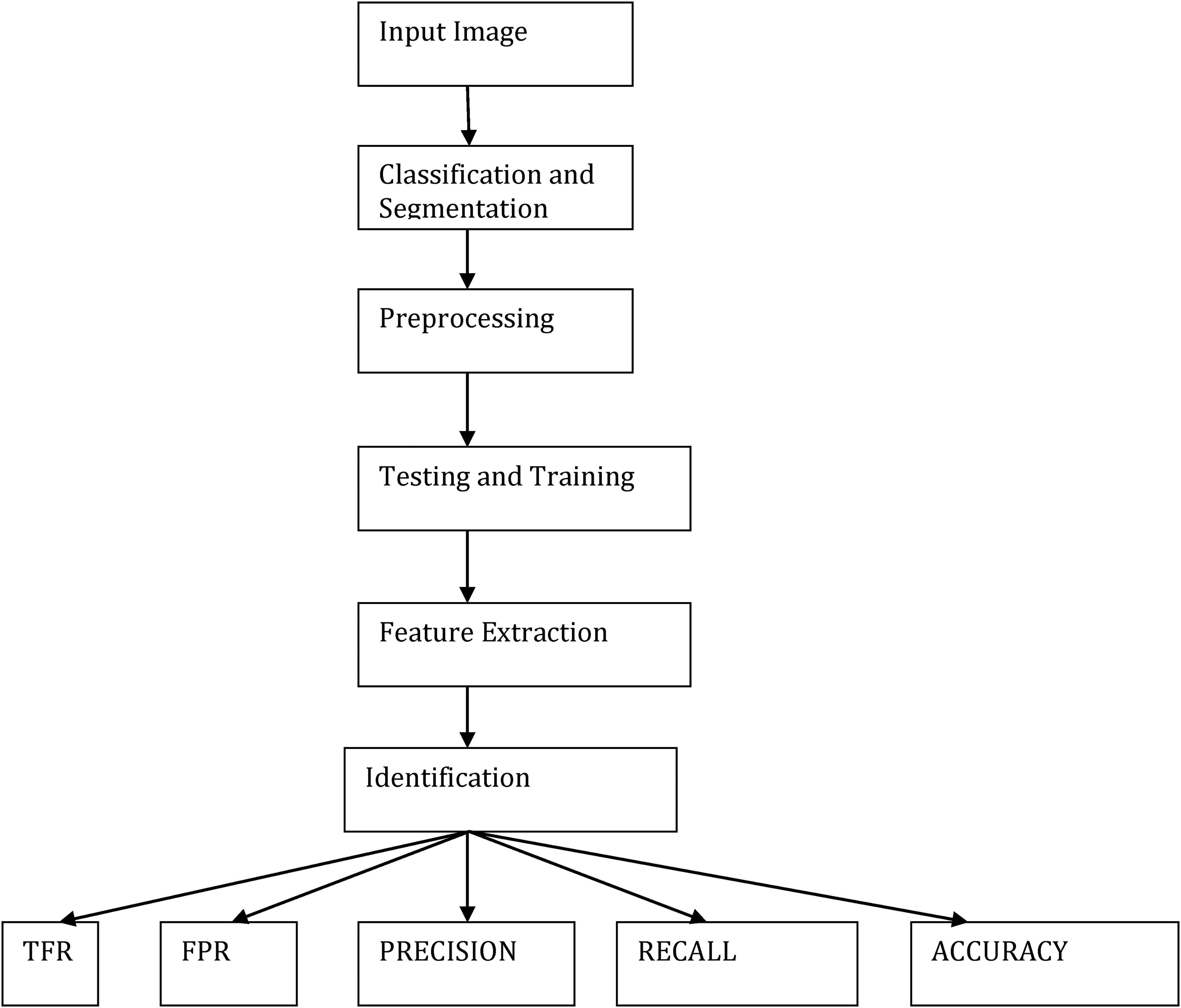
The methodology, as detailed in Figure 1, used several MATLAB techniques to obtain the aforementioned findings. We discovered this finding solely to pinpoint the precise location of tumors in real patients’ MRI pictures. There are also additional approaches to segmentation available. All of these techniques employ various MATLAB algorithms to identify tumors. The future of this profession is quite bright. If this study continues, we may use image processing methods to determine the kind, size, and stage of a cancer. When cells grow and divide in ways that don't make sense, it may lead to cancer. A brain tumour refers to a mass of these abnormally proliferating and dividing cells within the brain. Although they are uncommon, brain tumours are among the most lethal forms of cancer.We can classify brain tumours as primary or metastatic based on their initial origin. Primary brain tumors derive their cells from brain tissue. On the other hand, metastatic ones might develop in any place of the body and subsequently move to the brain. Glial cells give rise to gliomas, a kind of brain cancer. These are the most prevalent kinds of brain tumours under investigation at the moment.19–23
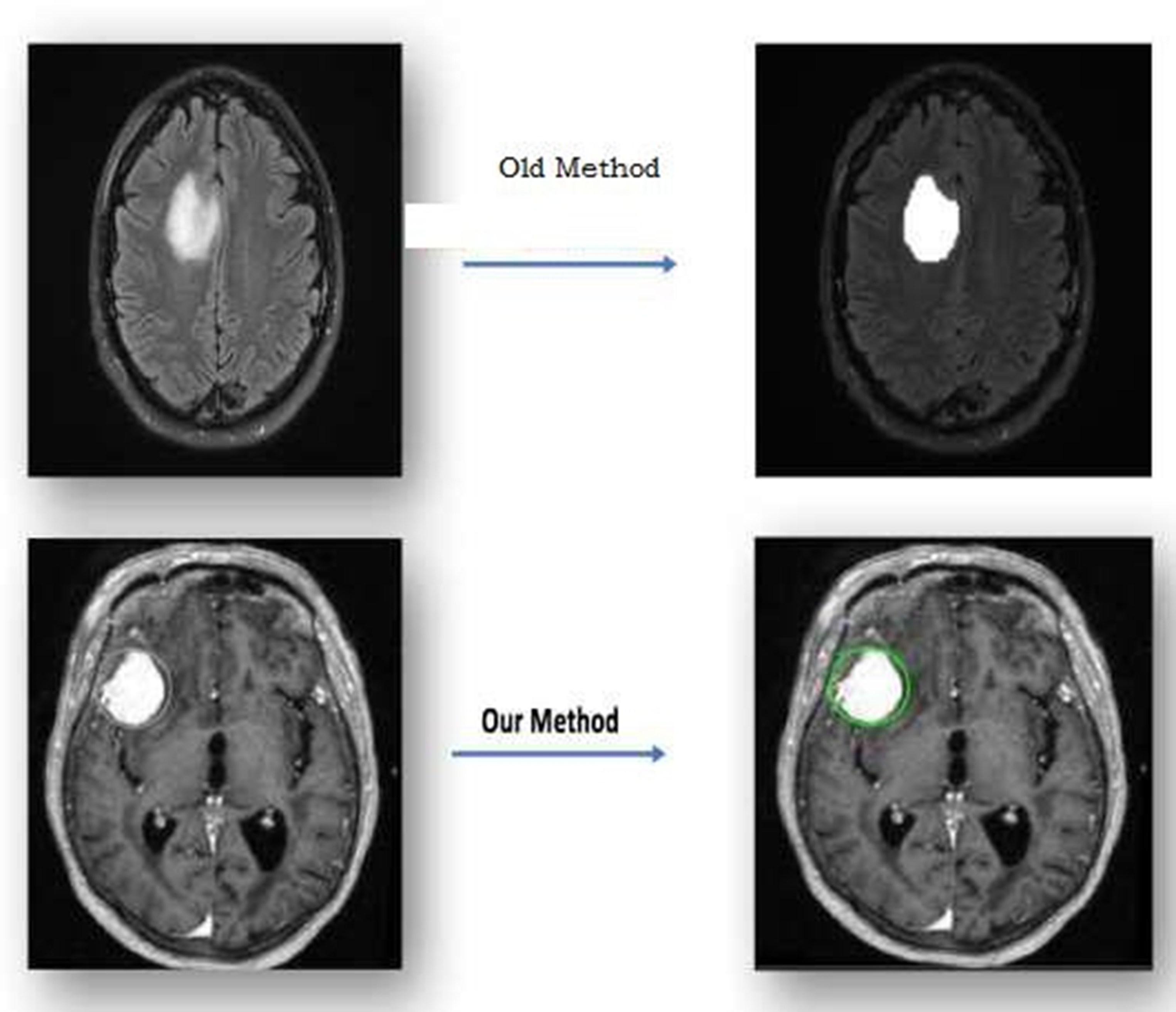
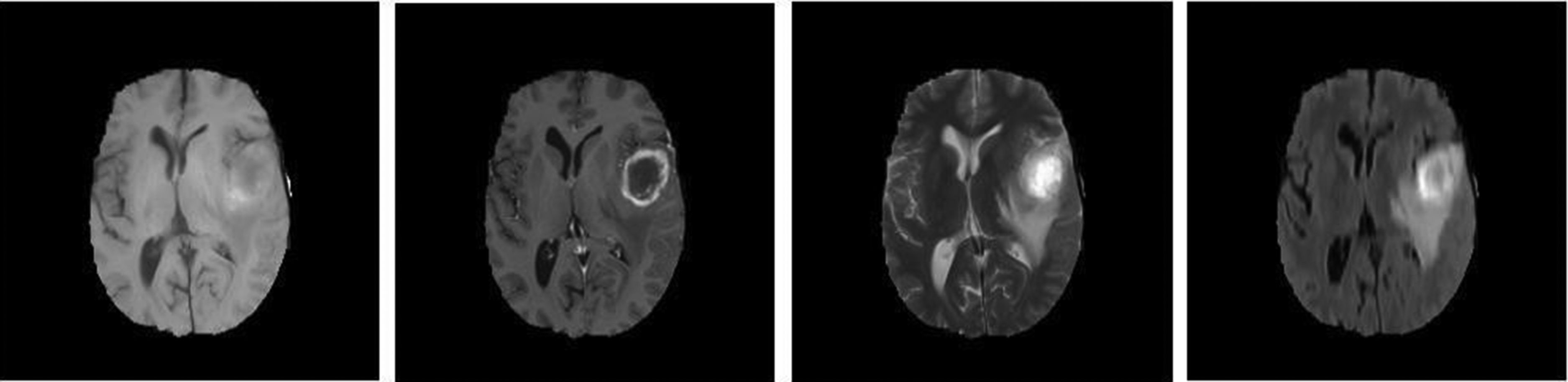
Proposed work sample.
Gliomas are a broad term for a variety of glioma forms, ranging from low-grade gliomas, such as oligodendrogliomas and astrocytomas, to high-grade (grade IV) glioblastoma multiforme (GBM), the most common primary malignant brain tumor and the most aggressive. Radiation treatment, chemotherapy, and surgery typically treat gliomas. Improving treatment options requires early detection of gliomas.Imaging methods like computed tomography (CT), single-photon emission computed tomography (SPECT), positron emission tomography (PET), magnetic resonance spectroscopy (MRS), and magnetic resonance imaging (MRI) can help doctors learn important things about brain tumours, like their shape, size, location, and metabolism. This aids physicians in making diagnoses. Even though doctors combine these modalities to acquire the most thorough information regarding brain tumours, MRI is considered the best method due to its simplicity and ability to show soft tissues well. An actual non-invasive imaging method is magnetic resonance imaging (MRI). Radiofrequency pulses excite target tissues, producing pictures of their interiors using a powerful magnetic field. By varying the excitation and repetition periods during picture capture, one can produce images with distinct MRI sequences. These various MRI modalities provide distinct tissue contrast images that provide crucial structural details and enable the diagnosis and segmentation of tumors. There are four main types of MRI used to find gliomas: T1-weighted MRI (T1), T2-weighted MRI (T2), T1-weighted MRI with gadolinium contrast enhancement (T1-Gd), and Fluid Attenuated Inversion Recovery (FLAIR) (see Figure 1).
MRI acquisition creates about 150 slices of 2D pictures, which vary from device to device and display the 3D volume of the brain. Additionally, the integration of slices from necessary standard modalities for diagnosis transforms the data into a complex and rich representation.
While T2 images identify oedema, which appears as a bright spot on the image, T1 scans often identify healthy tissue. On T1-Gd images, it's simple to see the edge of the tumour because of the strong signal of the gadolinium ions that have built up in the active cell zone of the tumour tissue. The less brilliant area of the tumour core may contain necrotic cells, as they do not react to the contrast agent. We can easily separate them from the active cell region of the sequence. FLAIR pictures turn off the signal of water molecules, making it difficult to distinguish between oedema and cerebrospinal fluid (CSF).24–28
Before commencing any treatment, we must slice the tumor into pieces to preserve healthy tissue while destroying and eliminating tumor cells. The process of identifying, characterising, and distinguishing brain cancer tissues from healthy brain tissues, such as grey matter (GM), white matter (WM), and CSF, is known as brain tumour segmentation. Currently, the clinic performs this task by manually annotating and separating a large number of multimodal MRI images.
Billion cells make up the brain, one of the body's most vital organs. When cells divide without instructions, a group of abnormal cells known as a tumour forms. We mostly use brain MRI images to identify tumours and understand their growth. Typically, doctors use this information to identify and treat tumours. The MRI image tells you more about a medical image than either the CT or ultrasound image. On the other hand, neural networks (NN) and support vector machines (SVM) have become the most common ways to implement them well in the last few years. But recently, deep learning (DL) models have started a new trend in machine learning. This is because the deep architecture can represent complex relationships well without needing a large number of nodes, like K-Nearest Neighbour (KNN) and Support Vector Machine (SVM). So, they quickly became the best in different areas of health informatics, such as medical image analysis, medical informatics, and bioinformatics.29–34
Because of this, many machine learning methods have been used successfully to spot a tumor. Random forests(RFs) and support vector machines were the most popular and well-known supervised classifiers that have been used to classifygliomas (SVMs).RFclassifier to build a model. They extracted the first-order operators (mean, standard deviation, maximum, minimum, median, Sobel, gradient), higher-order operators (Laplacian, difference of Gaussians, entropy, curves, kurtosis, skewness), texture features (Gabor filter), and spatial context features. All of these features are looked at to choose the important variable by choosing the right attributes. The researchers took 104 morphological and Gabor wavelet features, used an RF as a classifier, and then used neighbourhood-based postprocessing to improve the accuracy of the results. The method consists of three main steps: pre-processing and feature generation, which includes generating minimum, maximum, average, median, gradient, and Gabor wavelet features; training the RF to distinguish between normal and positive pixels; and post-processing, which utilizes the morphological phase to uniformly shape the detected lesions. The method utilizes the SVM classifier and the Berkeley wavelet transform to convert the spatial form into a frequency in the temporal domain.
They transformed the segmentation problem into a classification problem. They divided the pixels into normal and abnormal ones based on several features, such as intensity and texture, and they used an SVM as a classification algorithm. They came up with the idea of creating a spatial probability map for each type of tissue. This map divides the various types of tissue in a patient's brain into segments. We use spatial regularisation with a generative probabilistic model, which combines a healthy brain tumour atlas and a patient brain tumour atlas, to categorize brain tumours into clusters of images. A fuzzy logic-based hybrid kernel SVM to tell the difference between normal and abnormal MRI images. A study on how to classify tumours using Gabor wavelet analysis. They used Gaborwavelet analysis to extract the features, and then utilized Gabor filters and an SVM classifier to classify the tumour.35,36 Research suggests that deep learning could potentially overcome the challenges in detecting and treating brain tumours. One of the most advanced technical classification and detection methods, the segmentation technique, is widely known for its potential to eliminate aberrant tumour areas from the brain. When it comes to brain tumors, accurate, advanced A.I. and neural network classification algorithms may successfully accomplish early illness identification. The objectives of this research were to identify brain tumours using the VisualGeometryGroup (VGG16), implement a convolutional neural network (CNN) model architecture, and set parameters to optimize the model for this task. Additionally, the research developed a useful method for MRI-based brain tumour detection, which aids in making prompt, effective, and accurate decisions. We then categorised these maps to generate recommendations for tumour regions. We evaluated the performance by measuring the prediction accuracy. The report also includes future suggestions for the proposed research. 37 As the patient population has grown, the amount of data to manage has also increased, rendering outdated methods both costly and inefficient. Many scholars have looked at a variety of rapid and accurate methods for finding and classifying BTs. Recently, there has been a wider use of deep learning (DL) techniques to develop computer algorithms capable of swiftly and accurately identifying or segmenting BTs. We can use trained convolutional neural network (CNN) models with DL to identify BTs in medical pictures. Additionally, we created the BT segmentation dataset as a standard for creating and testing algorithms for BT segmentation and diagnosis. This dataset includes the suggested MRI images of BTs. 38
Proposed work
Researchers have become more interested in deep learning methods, especially convolutional neural networks (CNNs), after they did well in several object recognition and biological image segmentation challenges. In traditional classification methods, features are added by hand. CNNs, on the other hand, learn complex, representative features directly from the data. Because of this, most research on CNN-based brain tumour segmentation focuses on designing network architectures rather than using image processing topology features.
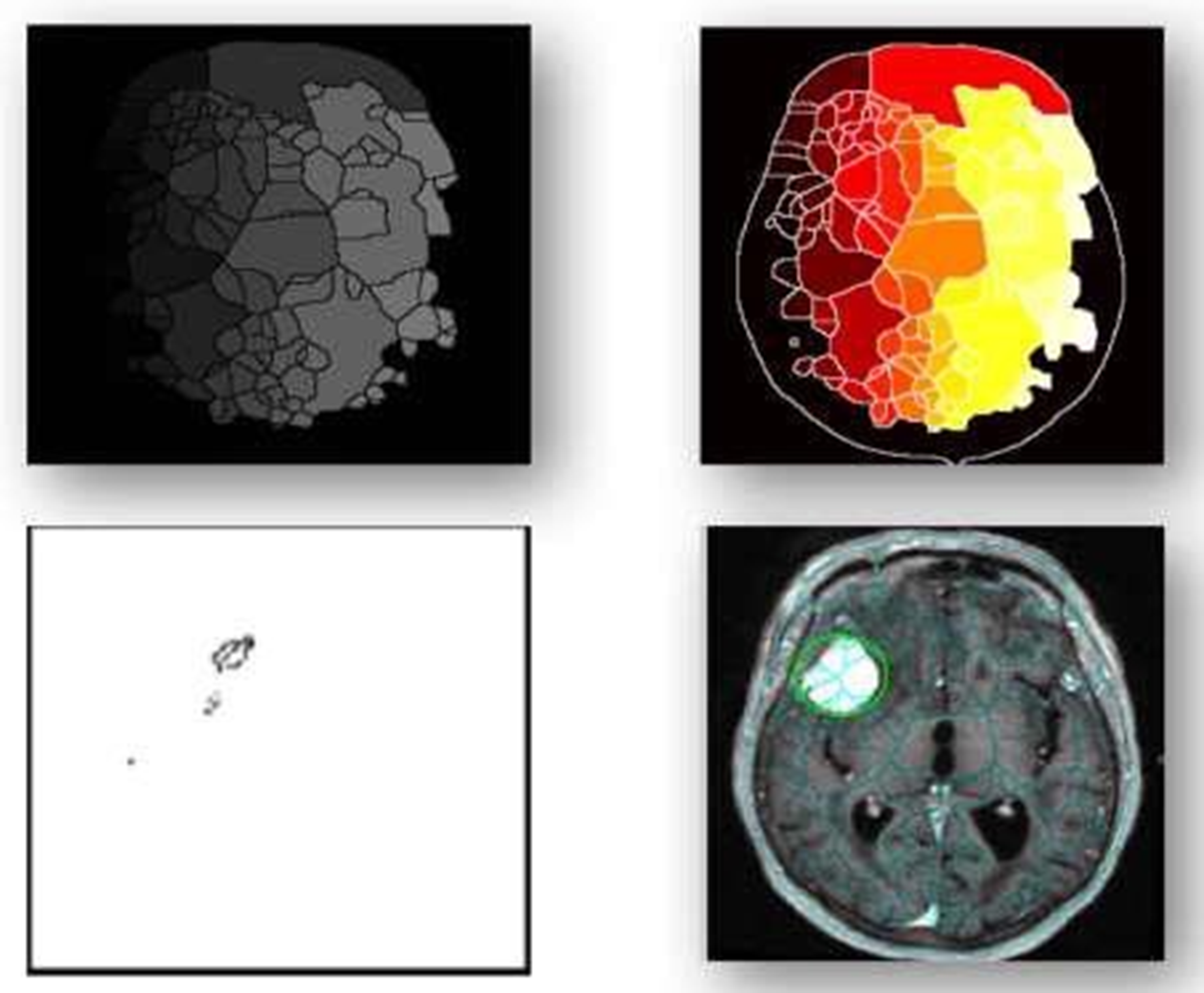
CNNsuseimagepatchesasinputsandusetrainableconvolutionalfiltersandlocalsubsamplingtogetahierarchyoffeaturesthatgetmorecomplicatedastheygoup.Despite the abundance of CNN-based brain tumour segmentation methods currently available, we will concentrate on these methods in this section due to their superior performance compared to more traditional approaches. For the multi-modal MRI glioma segmentation task, Urban et al. proposed a 3DCNN architecture. Multimodality 3D patches, which are made up of cubes of voxels, are taken from the different types of brain MRIs and fed into a CNNtop to change the tissue label of the cube's centre voxel Figure 2.
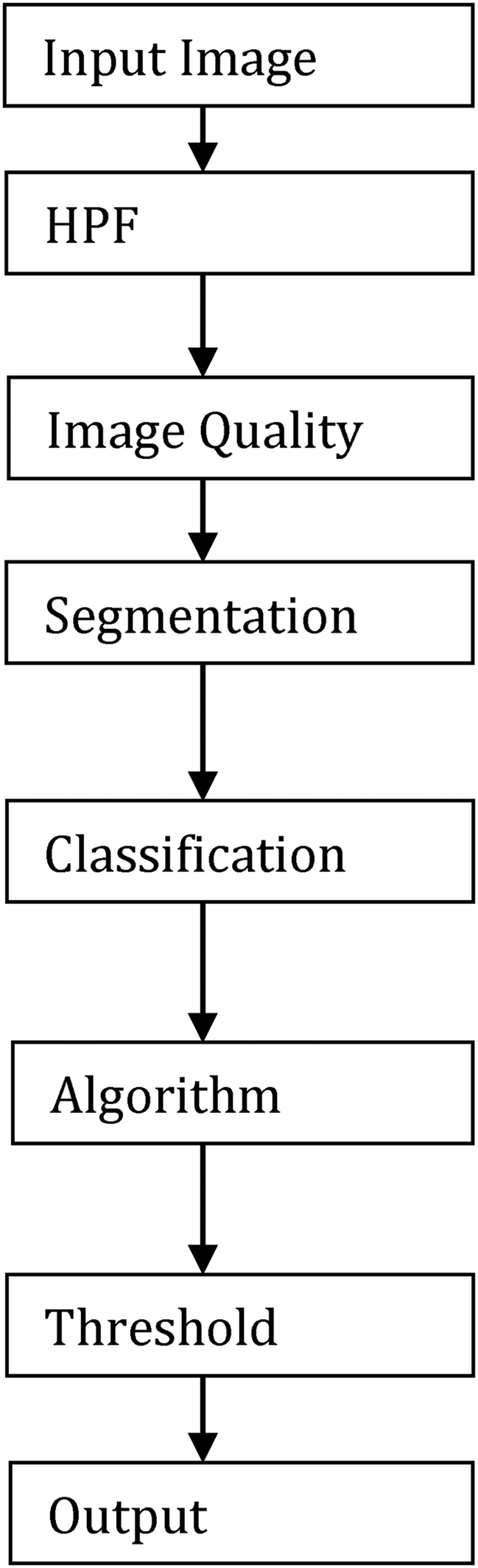
Flow chart of the image classification and segmentation.
Medical image processing has become one of the most important and dynamic areas of research, particularly in the medical field, since the 1990s. The advancement in imaging technologies and the application of computational methods has revolutionized how doctors diagnose, treat, and understand various diseases. These medical imaging techniques have extensive uses in multiple healthcare domains, ranging from early diagnosis to surgical planning and even post-operative monitoring. In addition, it is a crucial aspect of research, helping scientists and medical professionals better understand the human body and its functions.
One of the primary areas where medical images play a critical role is in the radiology department of hospitals. Radiology departments house sophisticated imaging equipment designed to capture biomedical images. These images, obtained through advanced medical imaging machines, provide detailed insights into the internal structure of the body, helping doctors and specialists assess the state of organs and tissues. Some of the most commonly used imaging techniques in radiology include X-ray, ultrasound, positron emission tomography (PET), computed tomography (CT), magnetic resonance imaging (MRI), and magnetic resonance angiography (MRA).
Biomedical imaging differs from the standard two-dimensional or colored medical images used in other fields, primarily because these images often capture information in 3D or 4D dimensions, offering more comprehensive views of internal body structures. They are particularly useful for identifying conditions such as tumors, fractures, organ abnormalities, and diseases like cancer, neurological disorders, and cardiovascular conditions. These techniques are typically non-invasive, meaning they don’t require surgical procedures to capture images of the internal body.
However, medical images are not always perfect. The captured images may have various issues such as noise, blurriness, low lighting, or lack of sharpness. These problems can make it difficult to detect the presence of tumors or abnormalities, potentially leading to diagnostic errors. To overcome these challenges, medical image processing techniques are employed to enhance the quality of the images before they are analyzed further. This process is a critical part of the medical imaging workflow and involves several techniques aimed at improving contrast, resolution, and clarity.
Once image quality is enhanced, the processed images can be used for various analytical tasks such as region-of-interest (ROI) segmentation, tumor size calculation, and the classification of image types. These operations are key to diagnosing conditions and determining treatment strategies. For example, in the case of cancer detection, machine learning algorithms can be applied to automatically identify and classify regions that are likely to be cancerous. These methods can also help in evaluating the size of tumors and predicting their growth over time, thereby assisting doctors in formulating appropriate treatment plans.
One of the most significant uses of medical image processing is in the detection and classification of tumors. Tumors are abnormal growths of tissue within the body, and they can be categorized into two main groups: benign and malignant. Benign tumors are non-cancerous, often growing slowly and rarely spreading to other parts of the body. In contrast, malignant tumors are cancerous, growing rapidly and spreading to nearby tissues, which can be life-threatening if left untreated. Accurate and early detection of these tumors is crucial for improving patient outcomes, as it allows doctors to intervene before the cancer spreads too widely.
Modern image processing methods, often powered by machine learning techniques such as Convolutional Neural Networks (CNNs), are widely used in the medical field for tumor detection and classification. These networks are specifically designed to automatically identify patterns in large datasets, such as images of tumors, and can outperform traditional diagnostic methods. CNNs have the ability to learn and adapt to new data, making them incredibly effective in detecting subtle patterns and abnormalities that may be difficult for human radiologists to spot. The application of CNNs has drastically improved the accuracy and speed of image analysis in medical imaging, reducing human error and ensuring more consistent results.
A typical CNN consists of multiple layers that progressively extract features from images. The network starts with simple features in the first layers, such as edges or textures, and gradually moves to more complex patterns in deeper layers, like shapes or specific structures. These features are then used to classify images into different categories, such as identifying whether a particular image contains a benign or malignant tumor. This process is often referred to as image classification.
In addition to classification, CNNs are also commonly used for image segmentation. Image segmentation is the process of dividing an image into distinct regions, such as identifying a tumor and separating it from surrounding tissues. This is particularly important for calculating the size of a tumor and determining its location within the body. 3D and 4D imaging techniques can further enhance the understanding of tumor growth by providing spatial context and time-based data, which is crucial for accurately tracking the progression of a tumor over time.
The role of CNNs and deep learning in medical image processing has made significant strides in recent years, offering new possibilities for diagnosing complex diseases. These algorithms have been particularly effective in identifying brain tumors and assessing the brain's anatomy. The brain is considered one of the most critical and intricate organs in the human body, and its study has been a major area of focus in medical imaging research. The brain is protected by the skull, a hard bone that serves as a barrier to injury, but inside, it houses billions of neurons, glial cells, and blood vessels that form the central nervous system (CNS).
The brain is composed of three primary components: grey matter (GM), white matter (WM), and cerebrospinal fluid (CSF). GM is the darker region in brain images and contains the neuronal cell bodies, while WM is the lighter region, consisting of myelinated axons that facilitate communication between different regions of the brain. The CSF is a clear fluid that surrounds the brain and spinal cord, providing cushioning and removing waste. The different properties of these tissues allow them to be easily distinguished in imaging studies.
When it comes to the brain and tumor analysis, CNNs are employed to segment the brain into its different components and identify any abnormal growths or masses. Tumors in the brain are particularly dangerous because they can interfere with brain function, leading to neurological issues, cognitive impairment, and even death. Therefore, the accurate detection of brain tumors is vital to initiating timely treatment, which may include surgery, radiation therapy, or chemotherapy.
The use of 3D and 4D imaging in conjunction with machine learning algorithms has also proven to be effective in understanding the growth of brain tumors. These imaging techniques provide a more detailed view of the tumor's size and location in three-dimensional space, allowing doctors to visualize how the tumor is affecting surrounding brain structures. In 4D imaging, time is also considered, which is helpful for tracking the tumor's progression over time and assessing the effectiveness of ongoing treatments Figure 3.
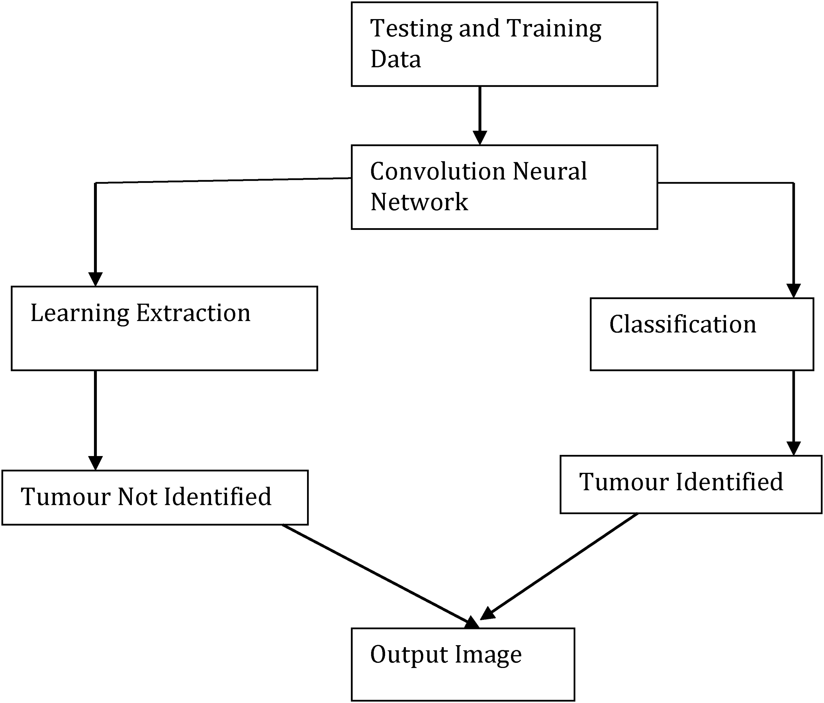
Block diagram of convolution neural network.
Since unsupervised classification doesn't need samples, it's relatively simple. We examine the picture using simple segmentation and classification techniques. Unsupervised approaches, such as K-mean, ISODATA, SOM, and several others, are employed. Additionally, there is a method known as “supervised classification,” which requires training set sample data. The three processes involved in this method are choosing the training region, creating a file containing the features of each class that are most similar to those in the training set, and finally categorising a picture. The two most popular supervised classification methods are maximum likelihood and minimum distance. SVM is yet another popular method for picture classification. Researchers have discovered that SVM performs best when a human performs the classification. However, SVM may also function as an unsupervised method in some circumstances. In this chapter, we discuss medical image analysis in depth, which is now a field of study. Researchers from a wide range of disciplines, including computer science, electrical and electronics engineering, biomedical engineering, and applied mathematics, have been examining this topic since the 1990s. Numerous methods already exist for analysing biomedical imaging. Preprocessing, which includes contrast correction, noise reduction, and picture sharpening, is the first stage in digital image processing. Figuring out how to automatically partition the ROI is the most crucial and challenging challenge in medical image processing. Researchers use segmentation to extract the area of interest from a single picture or a collection of volumetric images. Researchers have developed many methods to distinguish between the brain and tumour using MRI volumetric pictures, but most of them only work with 2D images and lack a 3D version. Classification is the process of determining the kind of object in computer vision and pattern recognition. Researchers employ the same concept as object recognition to determine the kind of brain cancer based on a picture of a tumor. They recommend well-known feature extraction techniques such as rotational invariant chain codes, LBP, LTP, HOG, GLCM, and geometrical features. One type of supervised learning in machine learning that makes use of labeled data is classification. Researchers have presented several methods for the classification of tumour types, including SVM, NB, ANN, KNN, and fuzzy classifiers. Each of these divisions has advantages and disadvantages (e.g., time complexity and accuracy). Most volume estimates use 2D MRI pictures; however, techniques like dpi (dots per inch) yield inaccurate results due to the varying pixel sizes on each display panel. We first see the segmentation in 3D before measuring the voxel size. In this manner, we can also use MRI DICOM volumetric data to precisely measure the brain and tumor. The MRI pictures must also be in 3D space in order to create a 3D image. We can create a 3D representation of the human body's organs to aid in illness diagnosis thanks to the thickness and pixel count of each MRI slice.
MR imaging is a widely used and significant biomedical imaging technology that produces three-dimensional (3D) pictures of soft, water-filled human cell grids. A single picture or a sequence of volumetric images produced by an MRI scanner may assist medical professionals (radiologists, surgeons, etc.) in diagnosing and treating patients. We will also examine and describe several picture segmentation techniques in our study. By removing undesirable portions of the cancer, image segmentation increases the accuracy of identifying the type of malignancy. It is believed that nearly all primary tumors, which are composed of brain cells, are benign. Failure to identify and treat the initial tumour within a specific timeframe may lead to its transformation into a malignant tumour. Therefore, a primary tumour may be benign or harmful. Tumours that develop outside of the brain are known as secondary tumours. They coat the tissues of the brain and develop slowly. Secondary tumours are always home to malignant tumours.The two primary categories of tumours are benign and malignant. The cells that make up benign tumours are not malignant. These soft issues are typically minor, develop gradually, and have no effect.
The training and testing stages are two components of CNN's brain tumour classification system. CNN uses labels such as “tumour” and “non-tumour brain image” to separate the quantity of pictures into distinct categories. In the training phase, we extract, preprocess, and classify features using the Loss function to establish a prediction model. First, label the training picture collection. During the preprocessing stage, we resize the pictures to change their dimensions. Finally, the convolutional neural network automatically classifies brain tumours. We source the brain picture dataset from ImageNet. An example of a pre-trained model is Image Net. You must train the whole layer, from start to finish, if you want to start from the first layer. Consequently, this process requires a significant amount of time. Its effectiveness will be affected. For classification phases, we employ a pre-trained model based on a brain dataset to prevent this type of issue. We will only use Python to train the final layer of the proposed CNN. We don't want to instruct everyone. Therefore, the suggested automated brain tumour classification system performs well and requires little computation time. We determine the loss function using the gradient descent approach. A scoring function converts the raw picture pixel into class scores. We can evaluate the quality of a given collection of parameters using a loss function. The degree of agreement between the induced scores and the ground truth labels in the training data determines this. Determining the loss function is crucial to improving the accuracy. The loss function is large when the precision is poor. Similarly, accuracy is high when the loss function is low. The gradient descent process determines the gradient value using the loss function. You must repeatedly assess the gradient value in order to determine the gradient of the loss function. We compare the accuracy of the current approach with all other state-of-the-art methods. We evaluate the performance of the suggested brain tumour classification scheme by calculating its training accuracy, validation accuracy, and validation loss. The present approach uses a classifier based on support vector machines (SVMs) to identify brain tumors. It requires output from feature extraction. We compute the accuracy based on the value of each feature, which determines the classification result. In SVM-based cancer and non-tumour detection, the calculation time is long and the accuracy is poor.
Malignant brain tumours are malignant brain tumours that cause significant brain tissue damage and spread to healthy brain tissue. Malignant tumors are large and spread rapidly. Determining the kind, grade, and stage of a brain tumour is difficult. Medical pictures help doctors see visible and invisible body parts. Physicians use these images to detect cancer and other health issues. Physicians maintain these images as part of the patient's medical history to monitor the tissues and determine if the condition is improving. Whether a medical picture is in color or grayscale depends on the physician's procedures and requirements. We use a magnetic field to create MRI pictures. The degree of contrast varies for every picture data set. We'll go into further depth regarding a few types of medical imaging below. One kind of radiography is computed tomography. A conventional X-ray machine produces a single picture. The radiologists’ requirements determine the number of images in each series created by a CT scan. CT scans can examine bones, teeth, and other metal-based hard elements of the body. Pregnant women and children should avoid x-rays due to their high frequency. The CT scanner uses the DICOM format, a 3D standard for medical imaging, to create pictures.
Magnetic power creates magnetic resonance images. A high-power magnetic and additional high-power magnetics are added in the machine. Helium gas, not actual magnets, provides the magnetic power in a 1.5-tesla MRI system. This approach is best suited for studying soft tissues like the brain, tumours, blood vessels, etc. The MRI also generates images in the DICOM format to evaluate the size of the tissues. Those who have a metal rod or other metallic item in their body should not see these photos; they are best suited for ladies and children. Picture segmentation is the process of breaking a picture up into segments according to how distinct they are, with each segment (pixel) having comparable characteristics. We use an information extraction and grouping technique from multi-band raster pictures. Pixels, subpixels, and objects are the three primary classification schemes. Pixel-wise image classification, further subdivided into three categories: software-calculated hybrid classification, unsupervised classification, and supervised classification (based on user guidelines), is the primary focus of this study. Despite the widespread use of each technique, object-based image analysis is relatively new and less common than the other two. High-resolution photos are the input for this technique.
Reliable feature extraction techniques are crucial for disease diagnosis and patient treatment strategies in biomedical image processing and computer vision systems. To understand, we assume that the image represents our data, which may be incomprehensible to a person with limited medical knowledge. We then process this picture data to extract specific types of information. Classifiers use these characteristics to develop methods for locating and identifying various illnesses and anomalies in the human body. A feature vector saves an image's characteristics, tags them, and feeds them into a classifier for training. Numerical values make up an image's features, and the vector that stores these characteristics is known as the features vector. Normal and tumour-containing image classification systems function similarly to computer vision and machine learning's object identification problems. CNNs are similar to more predictable multilayer perceptrons. Often, we refer to multilayer perceptrons as completely linked networks, in which every neuronee in one layer couples to every other neuronee in the subsequent layer. As a result of being “fully connected,” these networks have the tendency to match data too well. One popular method of regularization is to include a mechanism to gauge the magnitude of the weights in the loss function. CNN, however, approaches regularization differently. They construct more complicated patterns from smaller, simpler patterns by using the data's hierarchical structure.
The foundation of convolutional networks was biological processes. The connections between neurones resemble the structure of an animal's visual brain. Each cortical neurone stimulates only a limited portion of the visual field. We refer to this region as the receptive field. The receptive fields of several neurones overlap, allowing them to span the whole visual field. CNNs need less preprocessing than other image classification techniques. This suggests that the network adopts the filters manually configured in conventional techniques. When it comes to feature design, this independence from human labor and expertise is a significant benefit. Tasks such as image and video recognition, recommendation-making, image classification, medical image analysis, and natural language processing can utilize them.
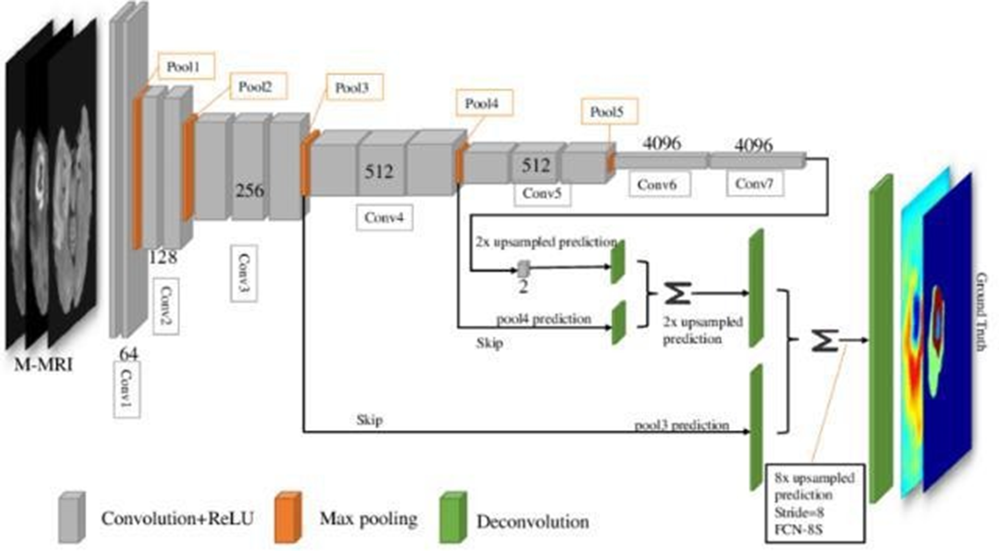
Image segmentation is the process of partitioning an image into different segments or regions, each corresponding to different structures or tissues within the body. In medical image processing, segmentation is critical for isolating regions of interest (ROIs) such as tumors, organs, or blood vessels. Accurate segmentation can help doctors identify abnormalities, plan treatments, and track disease progression over time. The simplest segmentation technique, where pixel values are compared against a threshold to determine if they belong to the tumor region or surrounding tissue. This method is particularly useful when the tumor has a clear boundary with contrasting intensity, but it may struggle in more complex cases This method starts with a seed point in the image and grows the region by adding neighboring pixels that are similar to the seed in terms of intensity or texture. Region growing works well when the regions of interest are homogeneous but can be sensitive to noise or other variations in the image. This technique treats the image as a topographic surface, where high-intensity regions are considered peaks and low-intensity regions are valleys. The algorithm simulates a flooding process, segmenting the image into distinct regions based on these intensity differences. A CNN-based architecture specifically designed for image segmentation tasks. U-Net consists of an encoder-decoder architecture with skip connections that help retain high-resolution features while reducing the spatial dimensions. U-Net has been highly successful in medical image segmentation, particularly for tasks like brain tumor segmentation in MRI scans. These networks consist entirely of convolutional layers, with no fully connected layers. FCNs are particularly effective for pixel-wise segmentation tasks, where the goal is to classify each pixel in the image into a particular category. Deep learning-based segmentation has significantly outperformed traditional methods in terms of accuracy, particularly when dealing with complex medical images like those of tumors, organs, or vascular structures. These models can handle a wide range of image variabilities, including different scanning protocols, patient positioning, and image noise.
Results and discussion
One of the study's initial objectives was to develop an automated method for detecting cancers in MRI slices. Depending on the kind of investigation, the number of MRI slices may increase or decrease. In our experiment, we examined two of the most advanced CNN techniques. A CNN model's two primary functions are feature extraction and classification, as we have previously discussed. We computed the true positive rate, false positive rate, precision, and recall to increase the classifier's accuracy, and we compared classifications using the confusion matrix. This research examines the use of deep learning CNN in the development of a computer-aided diagnostic system that can detect cancers in MRI images. It is believed that the safest and most efficient method of studying a concealed organ inside the body is using imaging technologies. Finding tumour slices using CNN requires filtering, feature extraction, and matching classification. We show the structure of the CNN-based tumour detection system. Figure 4 illustrates the wide range of parameters used in CNN training. We adjust CNN's parameters to identify the foundations for our models, enabling greater accuracy and faster processing. We implement our suggested approach for tumour slice identification using the MATLAB program. The suggested approach has an accuracy rate of 80% on the Googlenet model and 75% on the Alexnet model.
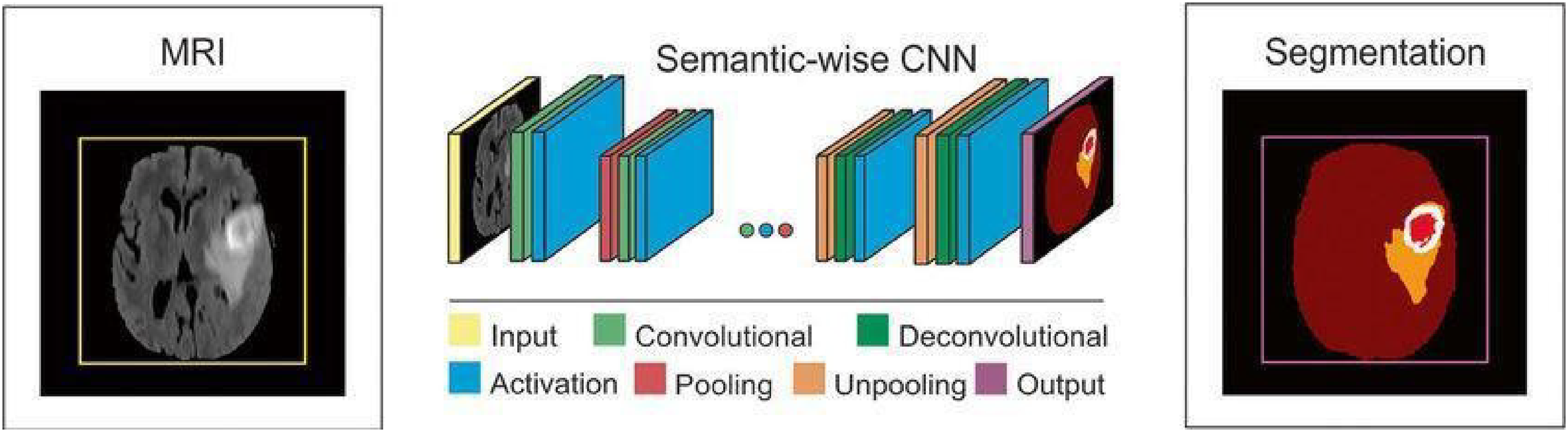
Block diagram of CNN model.
The primary objective of this study was to develop an automated method for detecting tumors in MRI slices using state-of-the-art deep learning techniques, specifically Convolutional Neural Networks (CNNs). This technique leverages the capabilities of CNNs to process medical imaging data, extract important features, and classify the images for tumor detection. MRI slices are cross-sectional images of the human body, often captured in a series for the purpose of diagnosing and monitoring various medical conditions. In this experiment, we focused on using CNNs to detect and classify brain tumors in these MRI slices, which may vary in number depending on the investigation being conducted.
Brain tumor detection is an important area of research in medical imaging, as it plays a key role in early diagnosis and treatment. The timely identification of tumors can significantly improve patient outcomes, particularly for aggressive forms of cancer. Manual detection of brain tumors by radiologists is a time-consuming task that requires careful inspection of each MRI slice. However, automation through CNNs can dramatically improve the speed and accuracy of tumor detection, reducing human error and enabling faster diagnoses.
CNNs consist of multiple layers, including convolutional layers, pooling layers, and fully connected layers. The convolutional layers are responsible for scanning the input image with filters (kernels) to identify key features, such as edges, textures, and other patterns in the MRI images. Each convolutional layer applies different filters to the image, enabling the network to learn more complex patterns at each successive layer. These features become increasingly abstract as the network deepens, allowing the CNN to learn and capture subtle and complex patterns that may be indicative of a tumor, even in noisy and complex medical images. After feature extraction, the CNN uses a series of fully connected layers to classify the image. The classification step involves taking the extracted features and determining whether the MRI slice contains a tumor or not. The fully connected layers compute a score for each class (e.g., “Tumor” or “Non-Tumor”), and the final classification is based on these scores. The CNN will output a binary classification (tumor vs. non-tumor) for each MRI slice, providing a decision that can help doctors assess whether further investigation or intervention is needed.
To measure the performance of the CNNs in detecting tumors, several evaluation metrics were employed:
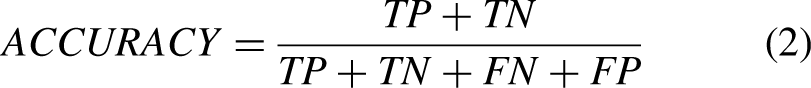
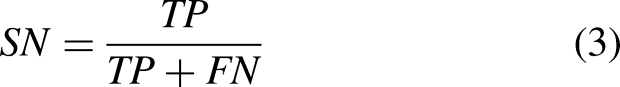
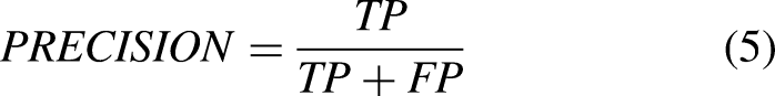
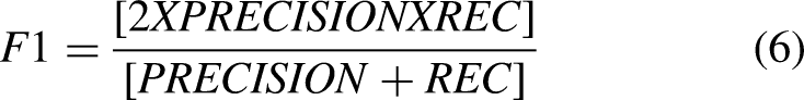
True Positive Rate (TPR): Also known as sensitivity or recall, this metric measures the proportion of actual tumors (true positives) that the CNN correctly identifies. A high TPR indicates that the model is effectively detecting the presence of tumors. False Positive Rate (FPR): The FPR measures the proportion of non-tumor MRI slices that are incorrectly classified as tumors. A low FPR is desirable, as it minimizes the number of false alarms or unnecessary interventions. Precision: Precision refers to the proportion of correctly identified tumor slices out of all slices that were predicted to contain a tumor. High precision means that the CNN is very accurate when it classifies an image as containing a tumor, reducing the number of false positives. Recall: Recall, which is synonymous with TPR, indicates the ability of the CNN to identify all relevant tumor images. A higher recall means that the model is effective in detecting as many tumor slices as possible, even if it means misclassifying some non-tumor images. F1 Score: The F1 score is the harmonic mean of precision and recall. It provides a single value that balances both the precision and recall of the model. This metric is useful when there is an uneven class distribution The confusion matrix was also used to further analyze the model's performance. This matrix provides a summary of the predicted classifications against the actual labels. By examining the confusion matrix, we can determine the number of true positives, false positives, true negatives, and false negatives, allowing us to calculate all the necessary evaluation metrics.
In order to support the findings of image classification investigations with scientific evidence, it is crucial to evaluate classification performance. Otherwise, the classification research would be incomplete and of poor academic quality. Researchers have long used a number of performance assessment measures in image classification investigations, which have evolved into standard metrics in related research. They are precision, sensitivity, specificity, and accuracy. This study employs the same criteria used as standard performance assessment metrics in image classification research to quantify the accuracy and reliability of the classification process. Additionally, we gauge the models’ effectiveness using the area of the receiver operation characteristic curve (ROC), also known as the AUC of the ROC curve. . The suggested MLS-CNN classification approach employs preprocessing, clustering, segmentation, feature extraction, and a classification process to determine if a brain tumor is malignant or not. Preprocessing is the first phase in the image analysis process, which smoothes, sharpens, and lowers input noise. Segmentation, the next phase, separates the targeted items and serves as the fundamental component of the classification system. After extracting the interesting items from the input, the system creates certain characteristics and uses them to classify objects. Adding local or global pooling layers can accelerate convolutional networksPooling layers reduce the number of data dimensions by consolidating the outputs from clusters of neuronees in one layer into a single neurone in the subsequent layer. Local pooling brings together small clusters, often two by two. Global pooling affects every neurone in the convolutional layer. Pooling may also determine an average or a maximum. Maxpooling takes the highest value from each set of neurones in the layer below. We use the average value of a collection of neurones from the previous layer for average pooling.
The VGG-16 is utilised to extract characteristics for our investigation. One popular CNN-based model is VGG-16. It is very methodical and successful in the area of image classification since it was trained on massive datasets like ImageNet, which contains at least one million pictures. The Visual Geometry Group members Simonyan and Zisserman, who won first and second place in the 2014 ImageNet Competition's classification and localisation categories, respectively, were the first to propose the design of VGG-16. A million tagged photos are used to train the VGG-16 neural network, enabling it to classify images into 1000 distinct categories. It includes 42 layers in all, 18 of which have learnable properties. A rectified linear unit (ReLU) with the hidden layers, three fully linked layers, and thirteen convolution layers are present. Convolution layers in the standard VGG-16 model consist of three filters (small receptive field) with convolution stride and padding sizes of one pixel each. A max-pooling layer comes after each convolutional layer.
Figure 5 illustrates how the VGG-16 may process 224224 pictures before sending them to the first two convolutional layers. The 64-feature kernel filters that comprise the first two convolutional layers are 33 and have 1 pixel convolution thresholds and padding widths.The feature map's dimensions are 224 by 224 by 64, and it features a maxpooling layer with a kernel size of 2 by 2.We apply the max-pooling layer across a 22-kernel space with a 2-pixel border. This process slashes the size of the preceding layer's feature map, which was 112 × 112 × 128 pixels, in half. The output is passed to the third and fourth convolution layers, each of which contains 1243-by-3-dimensional feature kernel filters, after passing via the max-pooling layer.The output is sent via a second max-pooling layer, which is carried out across a space of 2 × 2 kernels and a pixel size of 2, after the third and fourth convolution layers.This creates a 56 × 56 × 256 feature map. The fifth, sixth, and seventh convolution layers—each with 256 3-by-3-pixel feature kernel filters—process the feature map. Following these layers, a second max-pooling is performed over a 2 by 2 kernel and pixel-size space to create a 28 by 28 by 512 feature map. The 8th through 13th convolution layers include 512 feature maps and 3 × 3 filters. The block diagram of VGC model is shown in Figure 5. The network then performs max-pooling layers across a 2 × 2 kernel space, with a step size of 1 pixel. The network's final set, which follows, consists of three fully connected (FC) layers that combine to form a 33 filter with 4098, 4098, and 1000 ReLU-activated units, respectively.
Block diagram of VGC 16model.
Brain tumour detection
CNN AND VGC MODEL 16
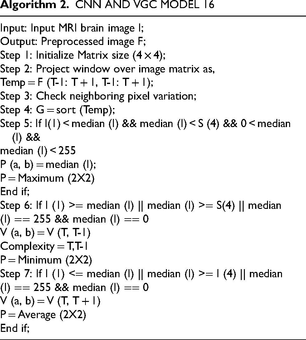
An intracranial solid tumour is an abnormal cell growth that occurs within the brain or central spinal canal.Tumors can cause various illnesses within the brain. Cerebral tumours are the same as brain tumours or cancers in the central canal of the spine. Cells split in an irregular and uncontrollable manner to create them. This often occurs in the brain, but it may also occur in lymphatic tissue, veins, cranial nerves, the meninges, the skull, the pituitary, or the spinal cord.Neurones or glial cells, comprising astrocytes, oligodendrocytes, and independent mal cells, can influence the mind itself. Diseases that began in other organs but progressed to the brain may also result in metastatic tumors. Given its invasiveness and stealth in the confined space of the intracranial cavity, any tumour has the potential to be fatal. However, brain tumours—especially lipomas, which are naturally benign—are not necessarily deadly, even if they may be incapacitating. Intracerebral neoplasms, another name for brain tumours, may be benign (not cancer-causing) or dangerous (producing cancer). However, the definitions of benign and dangerous brain neoplasms vary from those of benign and dangerous neoplasms in other body areas.Many factors, such as the type of tumour, its location, size, and stage, determine its risk level. Since the skull primarily protects the brain, the assembly of crucial instruments at the site of intracranial discomfort is the first indication of a tumour. Cancer typically manifests in this area when it is close enough to cause inexplicable symptoms. Although they may affect any portion of the brain, basic (genuine) brain tumours are often located in the front 66% of the cerebral side of the equator of adults and in the backcranial fossa of youngsters. The size (volume) and location of the tumor often make it straightforward to identify the signs and symptoms of brain tumors. When symptoms start to become apparent to the patient or others around them, it's a crucial stage in the process of diagnosing and treating cancer.
This algorithm has been constructed well.We collected the data from the Whole Brain Atlas website and used pre- and post-processing to prepare it for usage. We extracted features from photos using statistical feature analysis. We computed the features using the Haralick's feature equations and the spatial grey level dependency matrix (SGLD) of the pictures. We then selected the right and best left characteristics from Haralick's thirteen features to identify the tumour. We divided the photos into two categories for artificial neural networks: those with and without tumours. A feed-forward-back propagation neural network that learnt by being seen was used to do this. We trained the backpropagation network using some of its best characteristics as inputs and evaluated its performance.
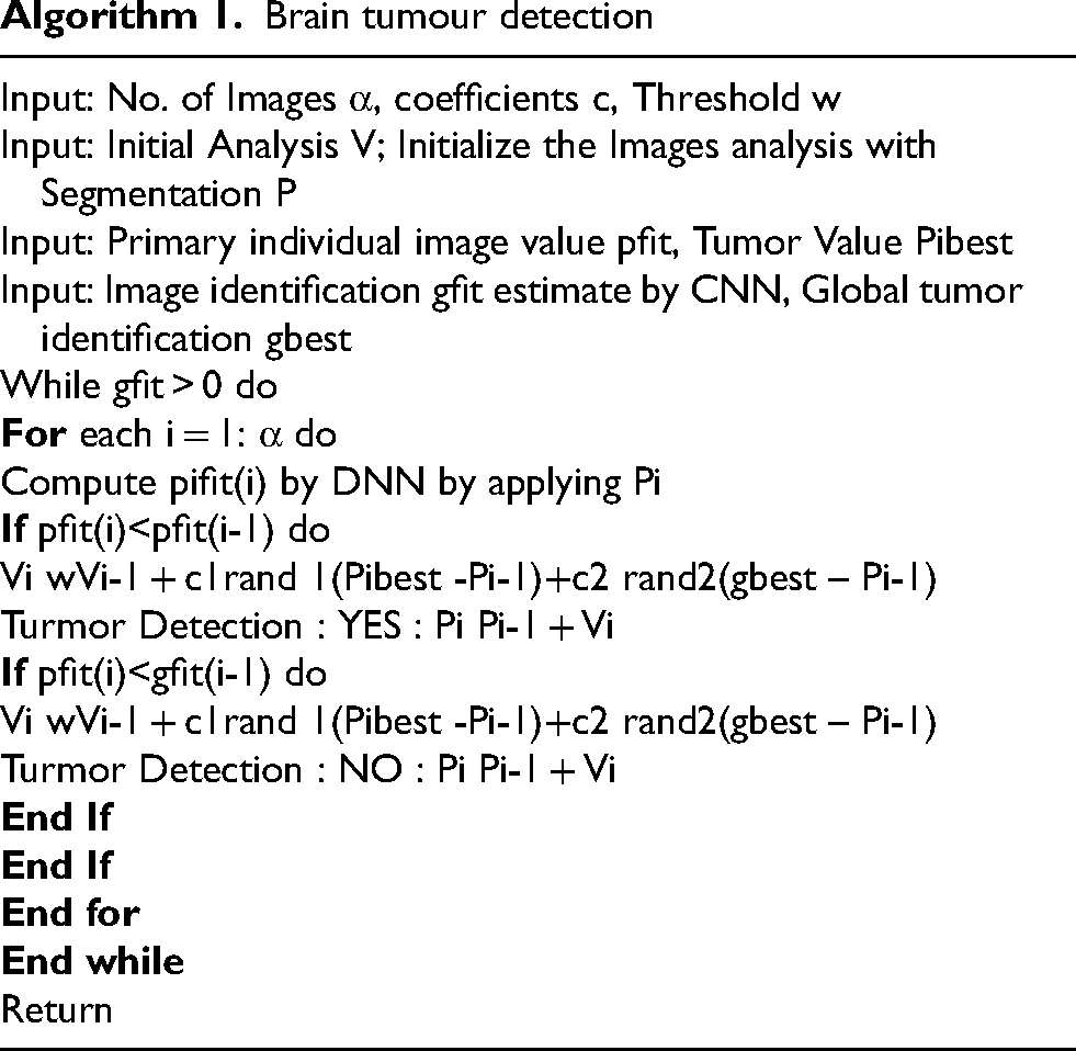
Last but not least, testing has shown that the suggested method, which is based on a back propagation network, performs best with 99% accuracy and 98.9% sensitivity. Additionally, a Graphic User Interface (GUI) window presented the investigation's outcomes step-by-step. We designed the system to be user-friendly by creating a Graphical User Interface (GUI). The suggested approach does a decent job at classifying brain tumour MRI images. To locate the cancer in MRI brain pictures, MATLAB is used to implement an integrated image processing technique that is based on a modified version of the texture detection algorithm's spatial gray-level dependency matrix (SGLD) of images. Algorithm 1 explains the brain algorithm. Algorithm 2 displays CNN's matrix model.
The task of automatically separating brain tumours to detect cancer presents a significant challenge. Recently, researchers have had a common platform to develop and objectively test new approaches with the current techniques because to the availability of public datasets and the well-recognised BRATS benchmark. In this study, we scrutinized the latest deep learning-based methods and presented a concise overview of the more conventional approaches. Given the strong reported performance, deep learning techniques may be able to accelerate the current state-of-the-art in glioma segmentation. When using standard automated glioma segmentation methods, it can be hard to pick features that are very good at representing the tumour or to turn past data into probabilistic maps. However, the benefit of convolutional neural networks (CNN) is that they can automatically learn representative complex characteristics from multi-modal MRI images for both healthy brain tissue and cancer tissue. Future advancements in CNN architectures and the addition of complementary data from other imaging modalities, such as Diffusion Tensor Imaging (DTI), Magnetic Resonance Spectroscopy (MRS), and Positron Emission Tomography (PET), could improve the current techniques and result in the creation of clinically viable automated gliomasegmentation methods for improved diagnosis.
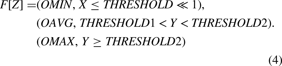
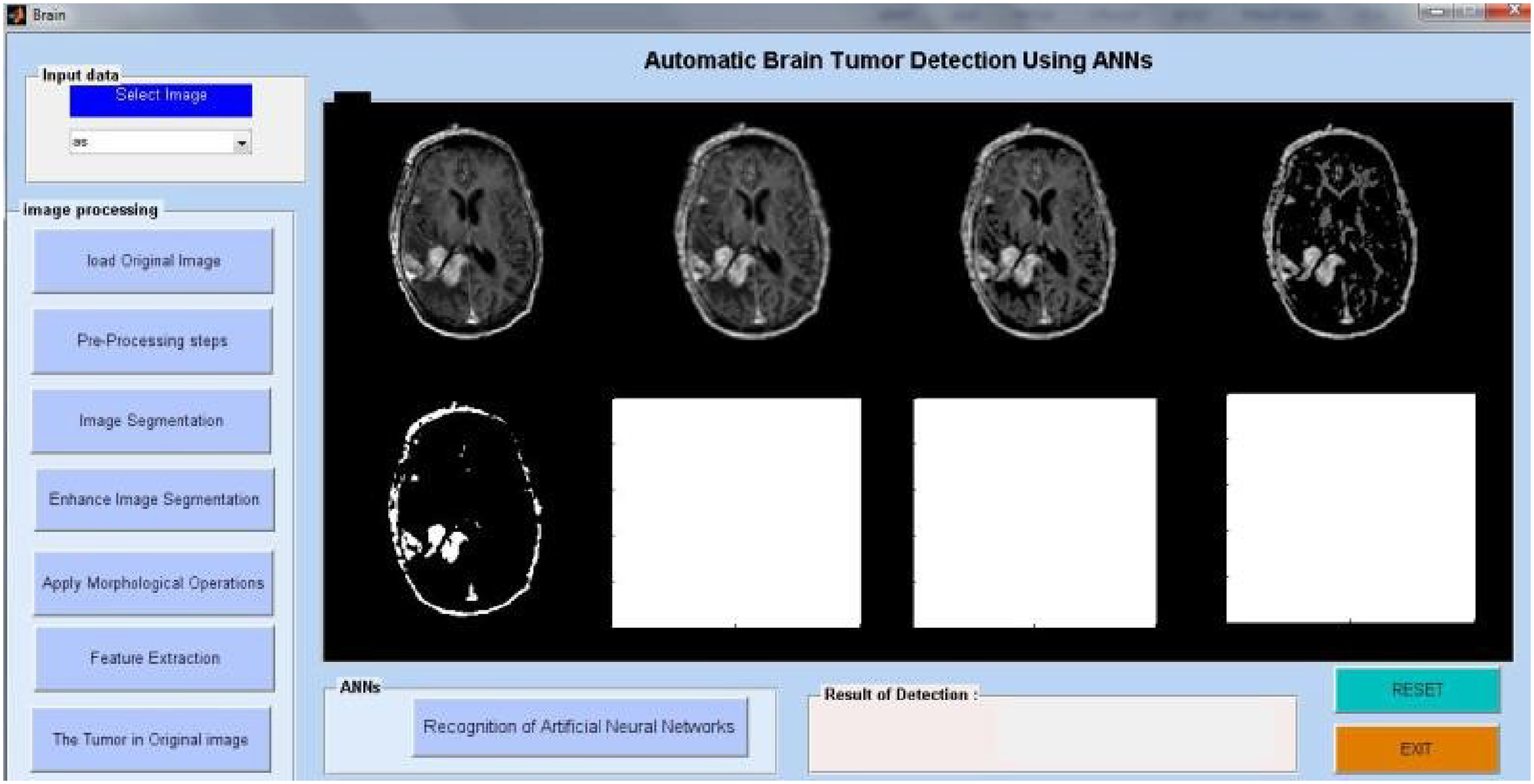
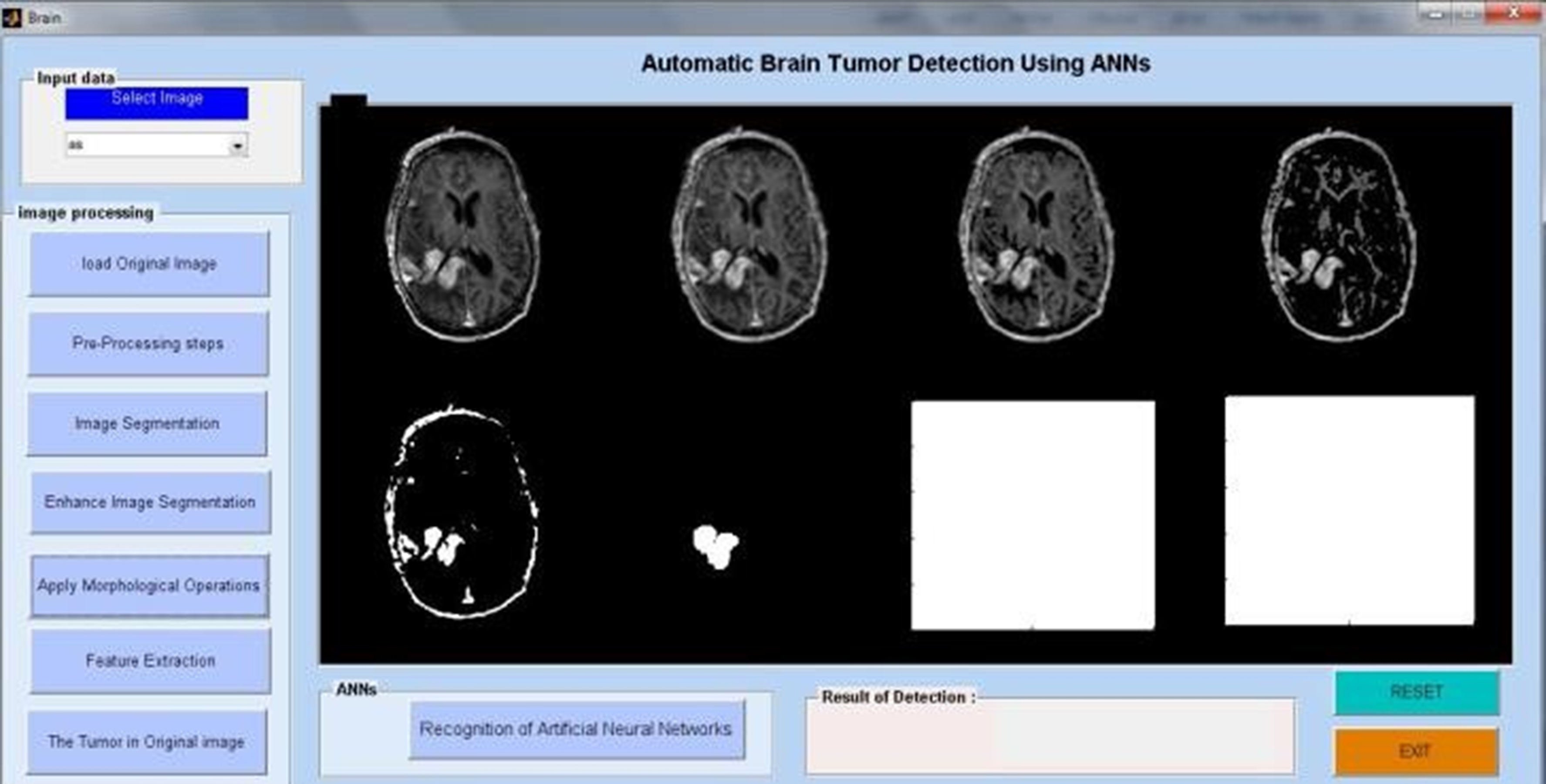
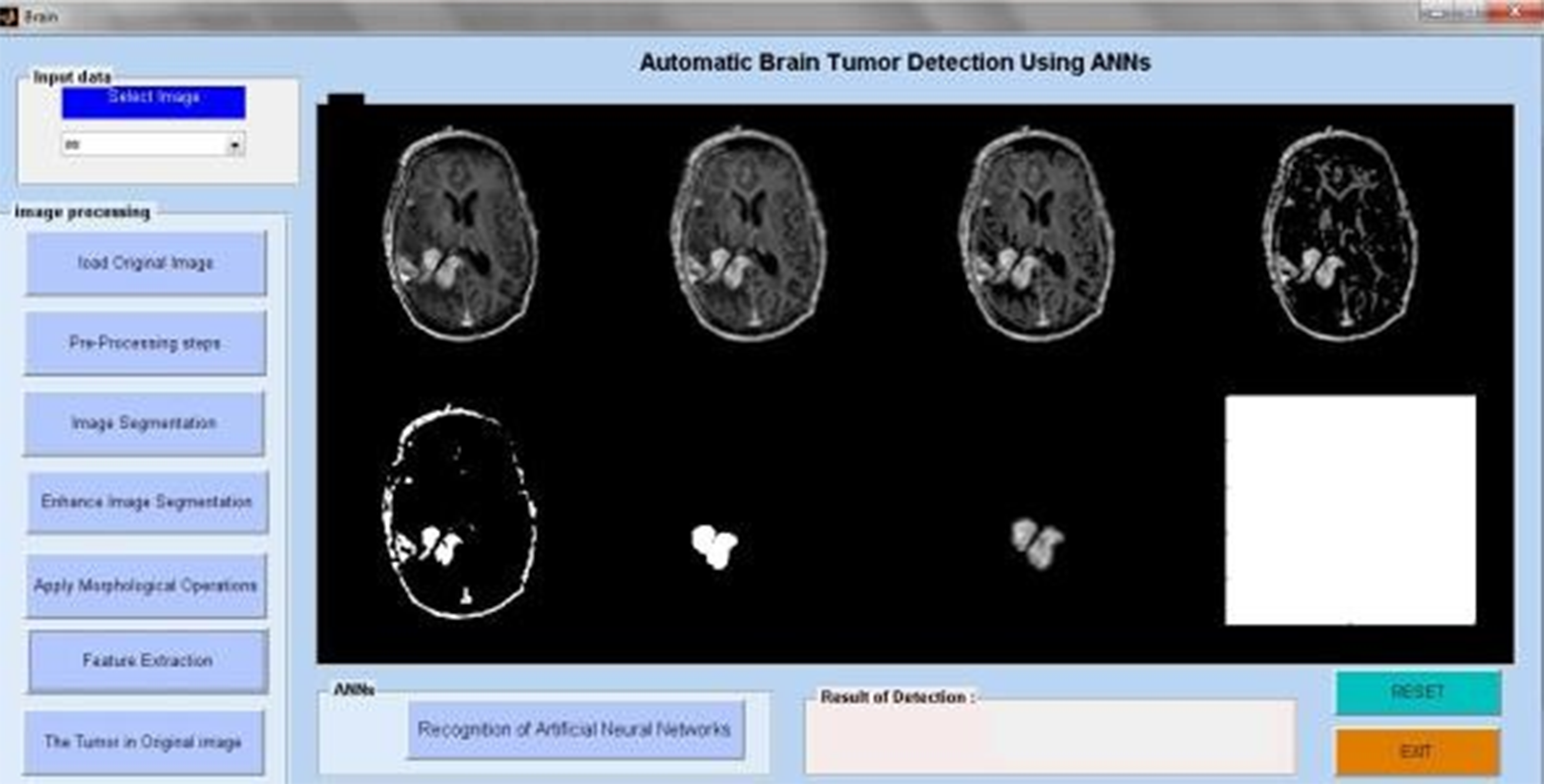
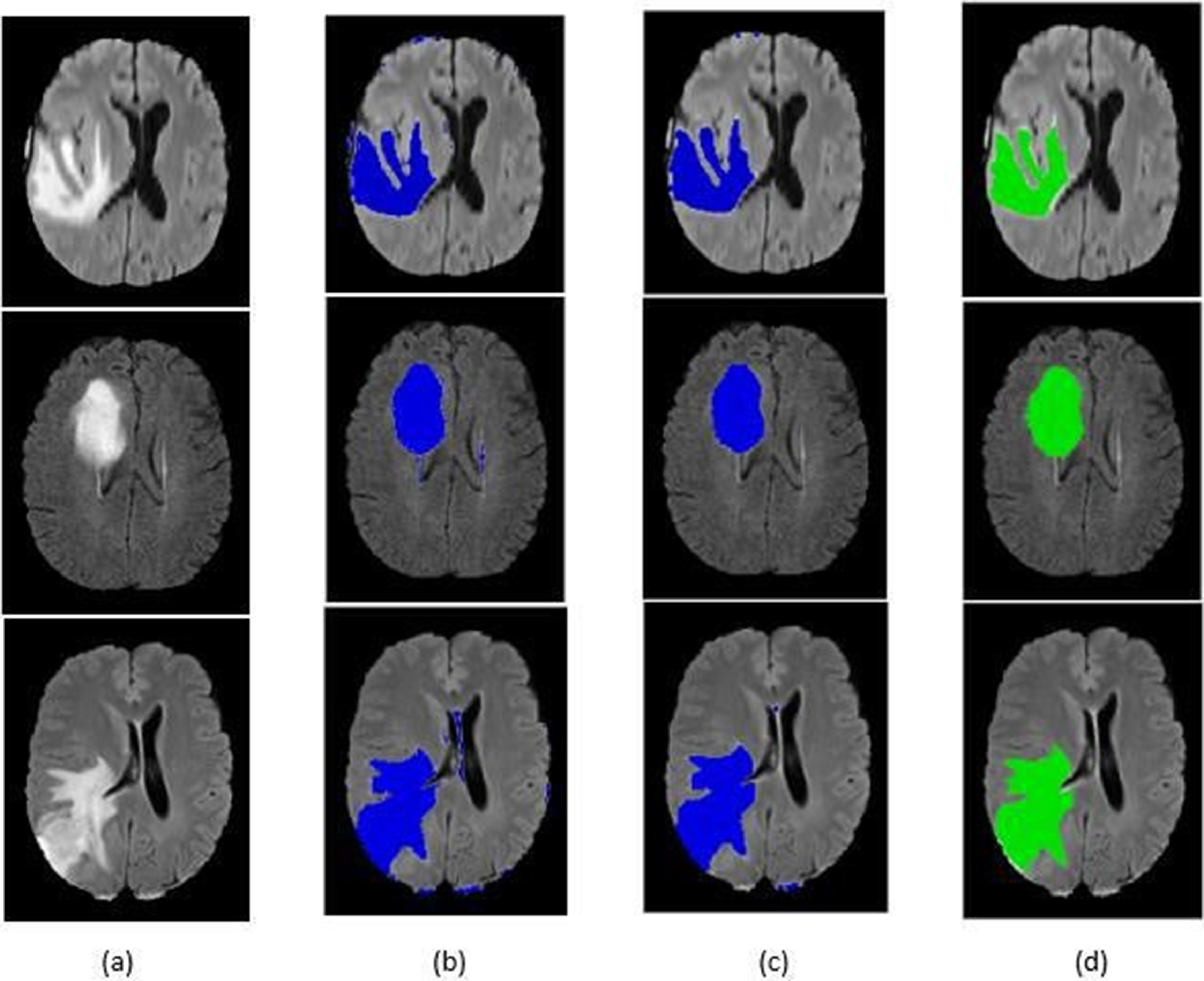
Researchers have looked at MRI scans using a variety of techniques to identify brain cancers. The automation of brain tumor identification and segmentation using MRI images is one of the most active research fields, according to our study. In this work, we examined the various entropy functions for identifying and classifying tumors in different MRI pictures. We determine the various threshold values based on the definition of entropy. The various entropy functions influence the threshold values, which in turn influence the segmented results. Figure 6 displays the different performance analyses of brain tumour detection. Figure 7 displays the preparation of the brain tumour. Figures 8 and 9 show the segmentation of brain tumours. The brain tumor's morphological operation is shown in Figure 10.
Comparative performance analysis of the proposed system.
MRI image preprocessing for tumor identification.
Tumor region identification in brain MRI.
MRI tumor region segmentation.
Morphological techniques for tumor detection.
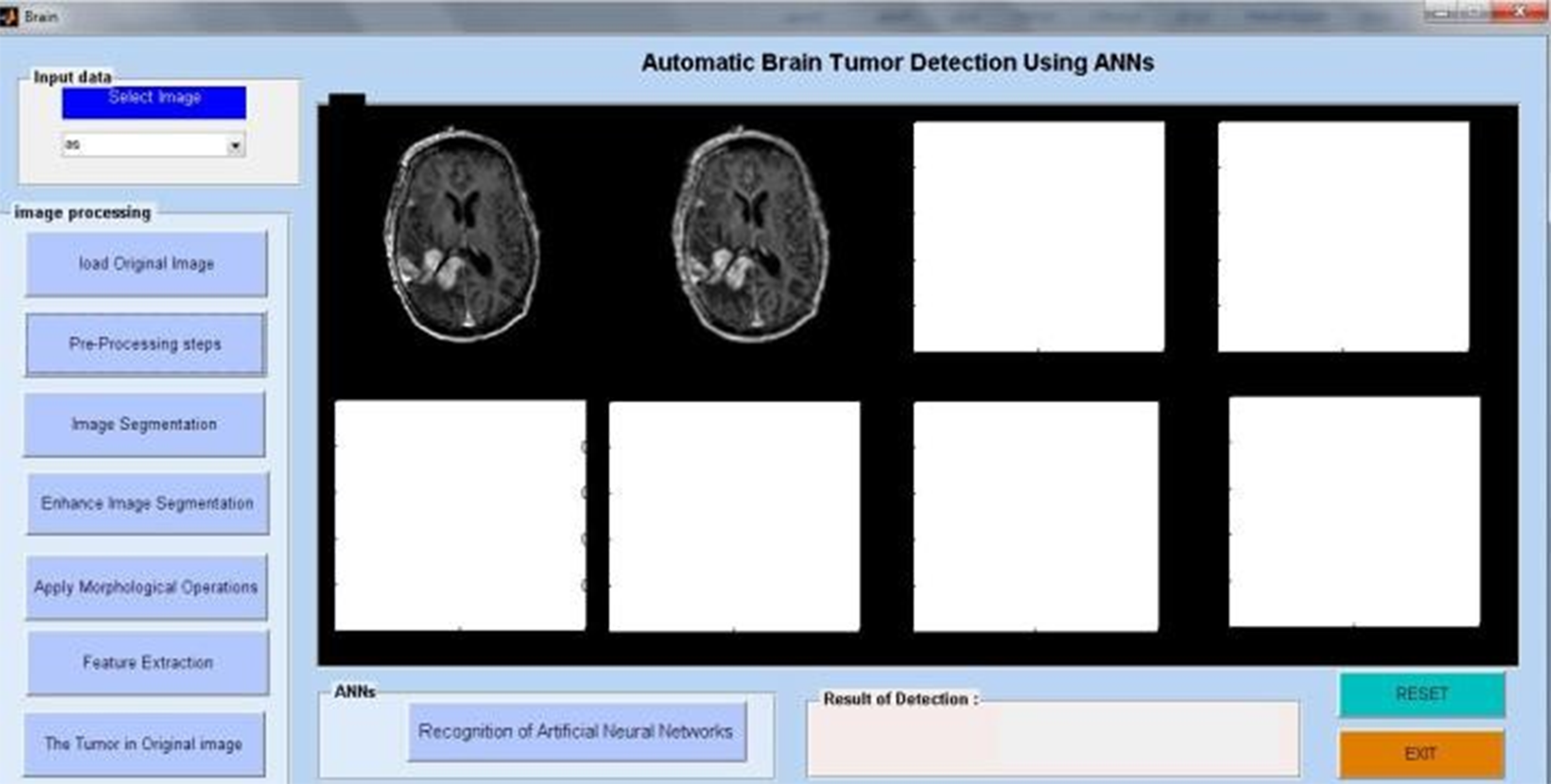
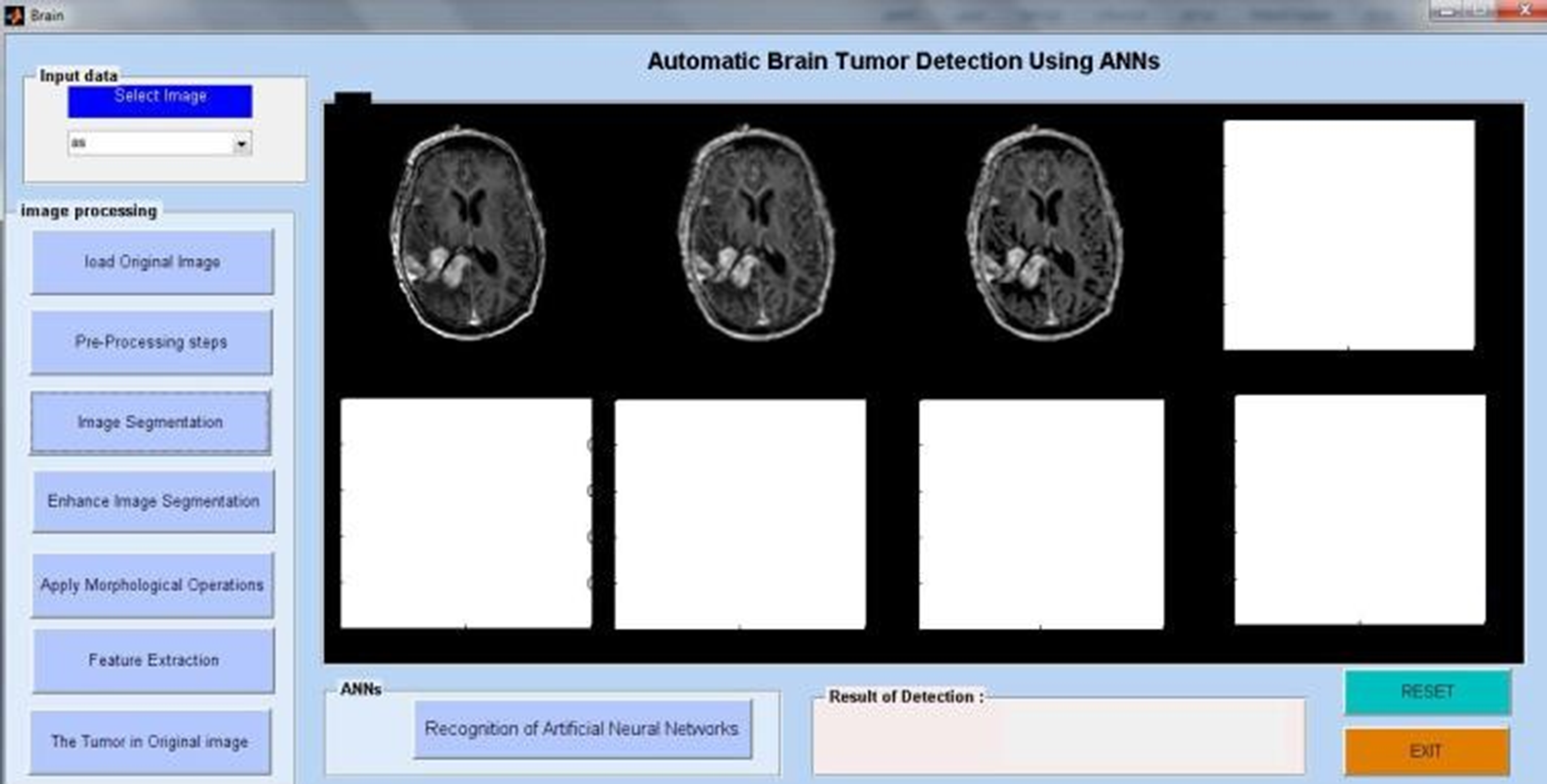
Using an artificial neural network algorithm, we analyze MRI pictures from several patients in the first phase to identify tumor blocks and categorize the types of cancer. Figure 11 illustrates the extraction of the brain tumor. Figure 12. The first image depicts the brain tumour. The proposed system consists of five key components. collection of data, Prior to processing, Divide the data, create a CNN model, train an epoch-specific deep neural network, and then classify it. We may use one of the several MRI images in the dataset as an input image. During pre-processing, we encode the label of an image and alter its size. In Figure 13, we divided the data into 88% training data and 40% testing data. Figure 14 displays the MRI modalities. Figure 15 displays the watershed picture. Figure 16 shows the progression of the brain tumour in the Annular Network. Figure 17 shows the segmentation of brain tumours. Figure 18 illustrates the augumentation of a brain tumour. Figure 19 displays the detection of a brain tumour. Next, train a deep neural network for epochs using a CNN model. We then categorised the picture as either “yes” or “no.” The outcome would be “yes” or “no” depending on whether the tumour was “yes” or “no.” One method of sharing information that reduces the number of this includes the amount of training data, the duration required to create deep learning models, and the associated costs. A previously trained model may teach a new model using transfer learning. There are several applications for transfer learning, including the classification of tumours, the prediction of software problems, the recognition of activities, and the classification of people's emotions. We contrasted the performance of the well-known transfer learning technique VGG16 with that of the suggested DeepCNN model.
Tumor image data analysis.
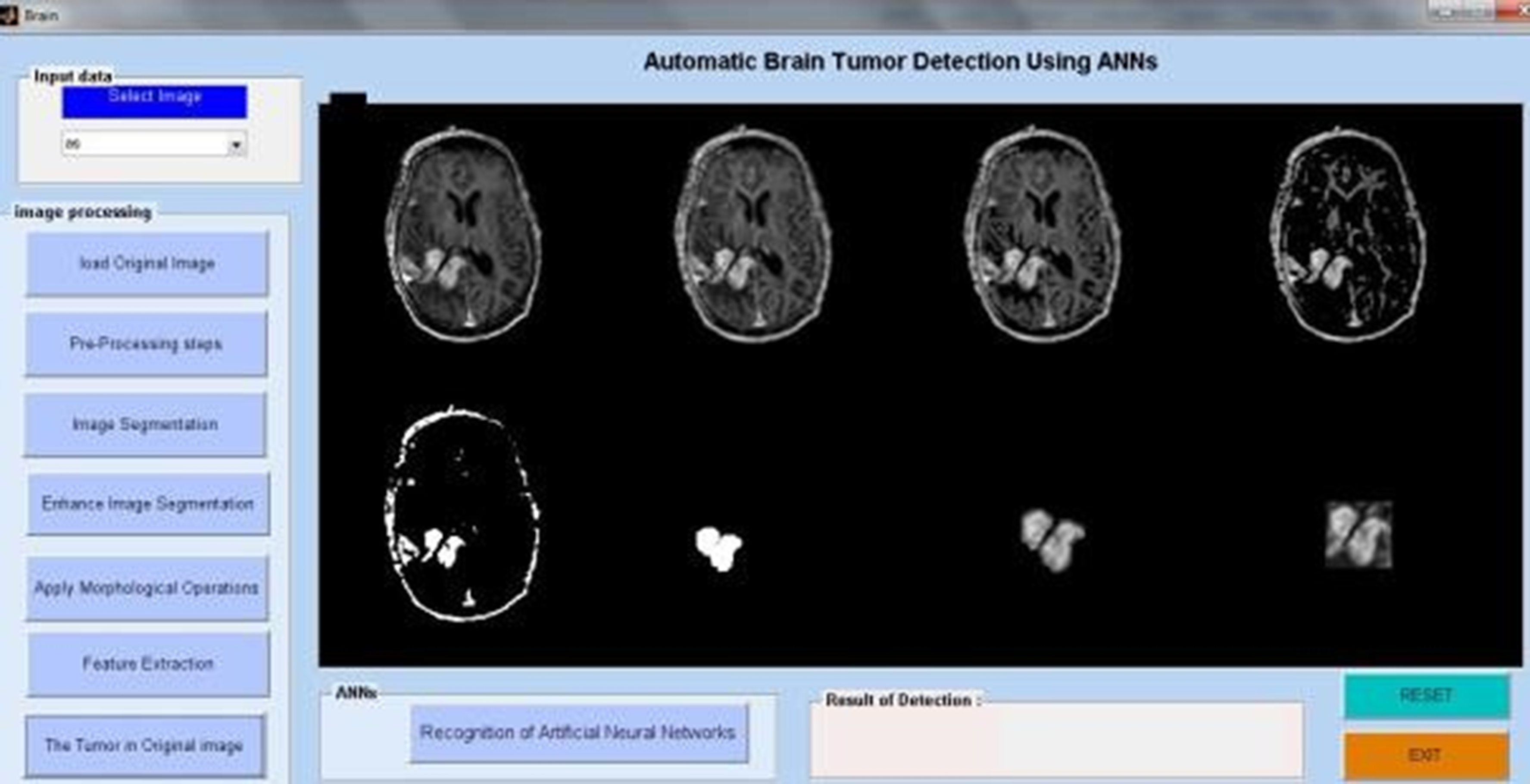
Tumor highlighted in original brain image.
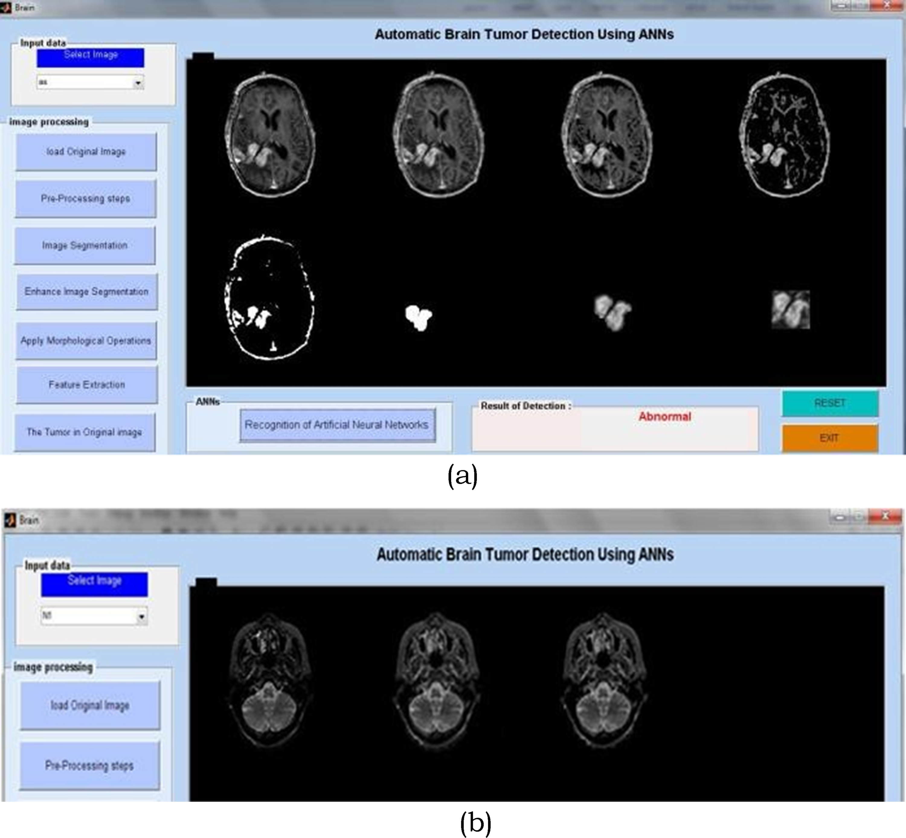
(a & b) Brain tumor detection using ANN.
MRI imaging modalities and protocols.
Watershed segmentation method.
Brain tumor analysis process using neural networks.
Brain tumor detection and isolation.
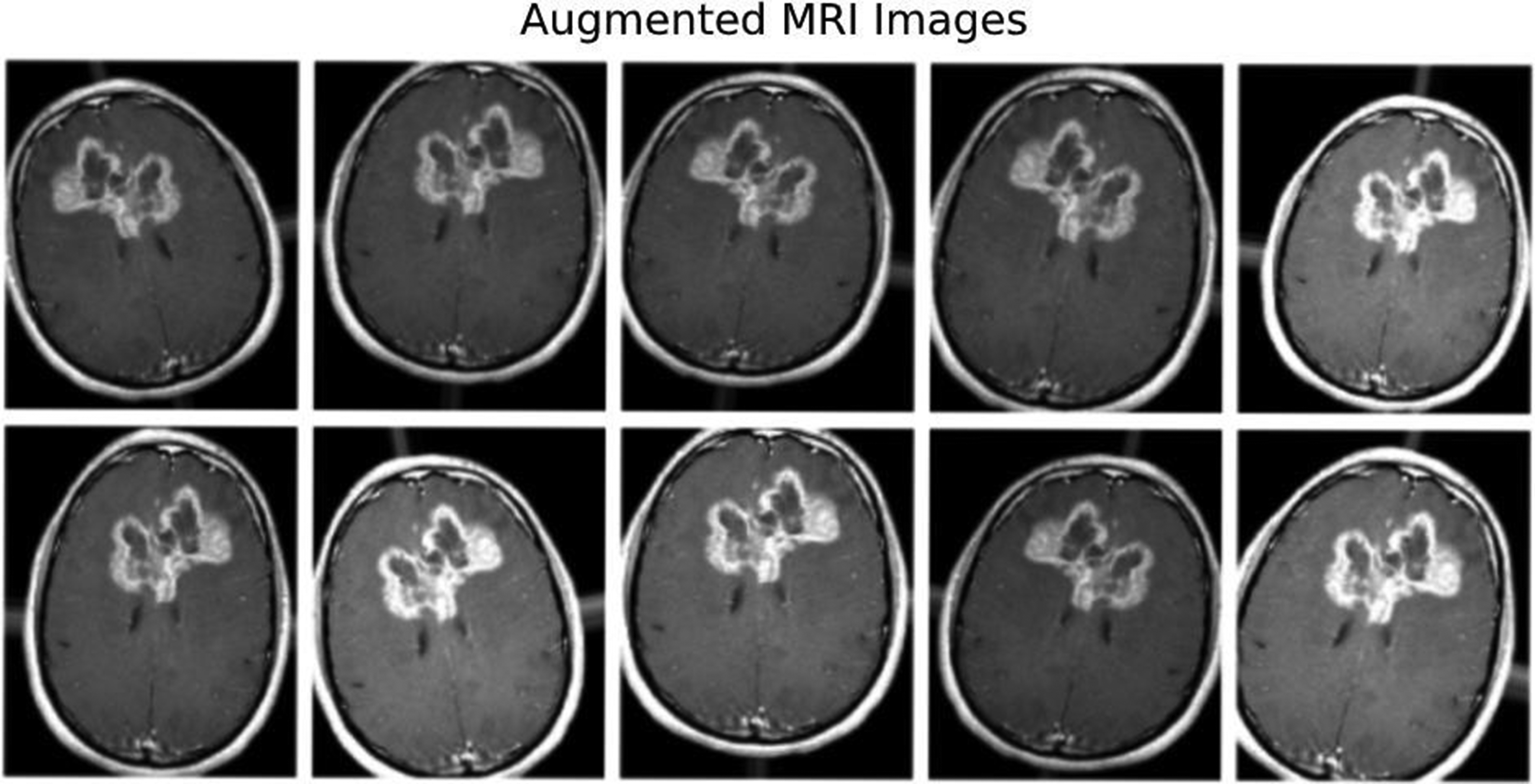
Augmented brain tumor analysis.
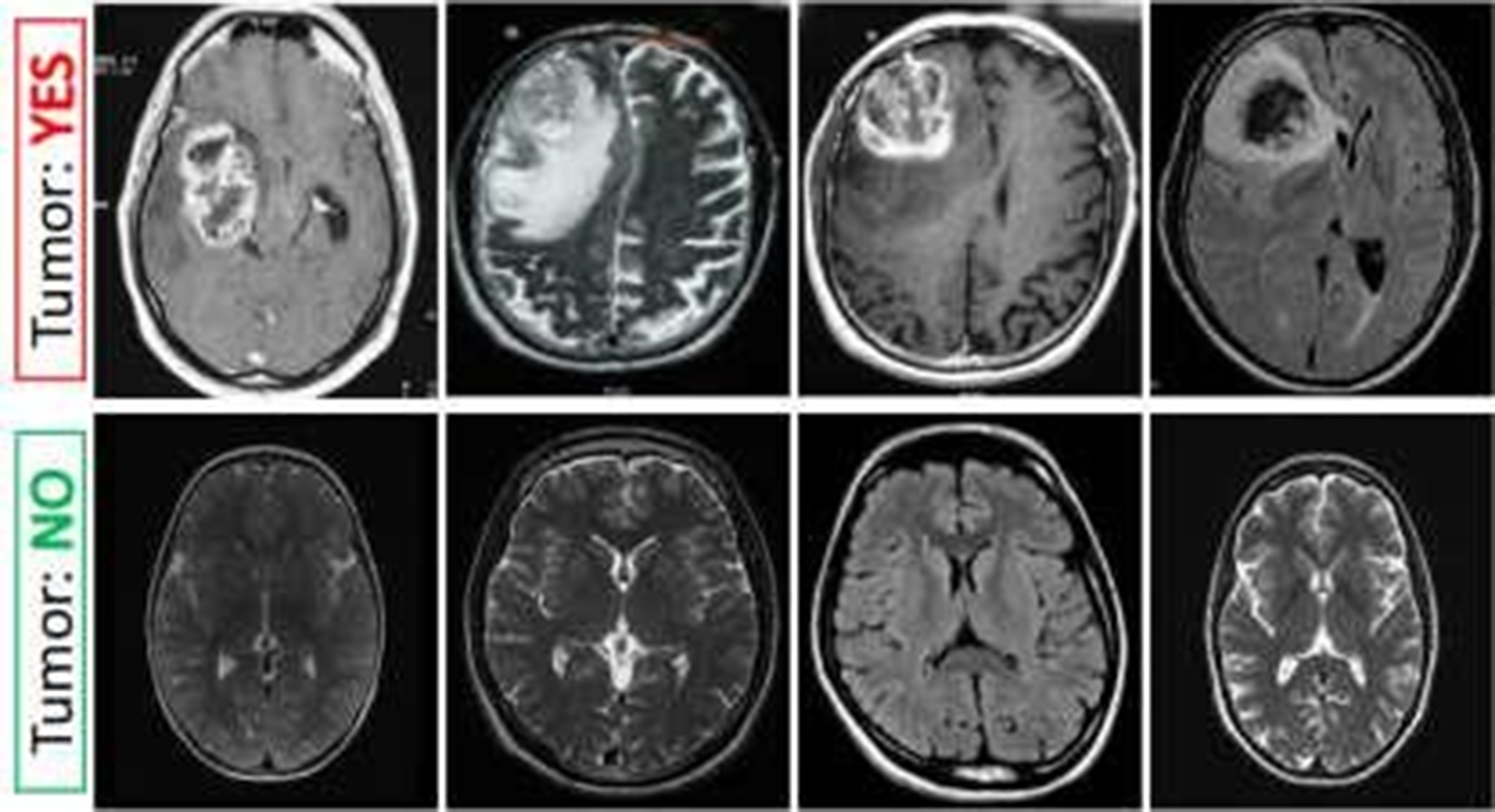
Detection of tumors in brain imaging.
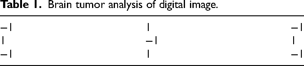
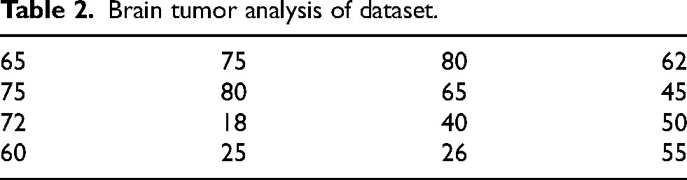
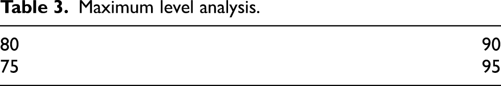
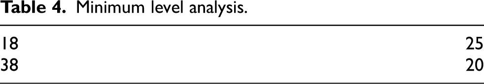
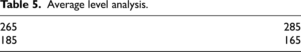
The study's objective is to develop a method for automatically identifying brain tumors in MRI data. Our proposed approach, based on the DCNN architecture, utilizes brain MRI scans. There are several phases in the proposed technique. Initially, the brain's MRI image serves as the “input” image. Once we have used picture thresholding and dilations to remove noise, the next step is to normalise the data. We process and supplement the gathered MRI pictures of the brain. We then scaled the photos for the model's input and sorted them into two groups—YES and NO—using a previously trained CNN named VGG-16. The ImageNet platform trained one variant of VGGNet, known as VGG-16. It is among the most sophisticated networks of image classifiers. This work involves creating a database using brain MRI images. The 253 raw photos come in a range of sizes. Table 1 displays the digital imaging analysis for the brain tumor. Table 2 displays the dataset's analysis of brain tumours. Table 3 displays the maximal brain tumour analysis. Table 4 displays a minimal analysis of brain tumors. Table 5 displays the typical brain tumour analysis.The images are from Kaggle's brain MRI datasets. We store them in JPG files. We separate the dataset into two groups, yes and no, based on the presence or absence of tumours. There are 98 images of healthy brains and 155 images of brain tumors, overall.
Brain tumor analysis of digital image.
Brain tumor analysis of dataset.
Maximum level analysis.
Minimum level analysis.
Average level analysis.
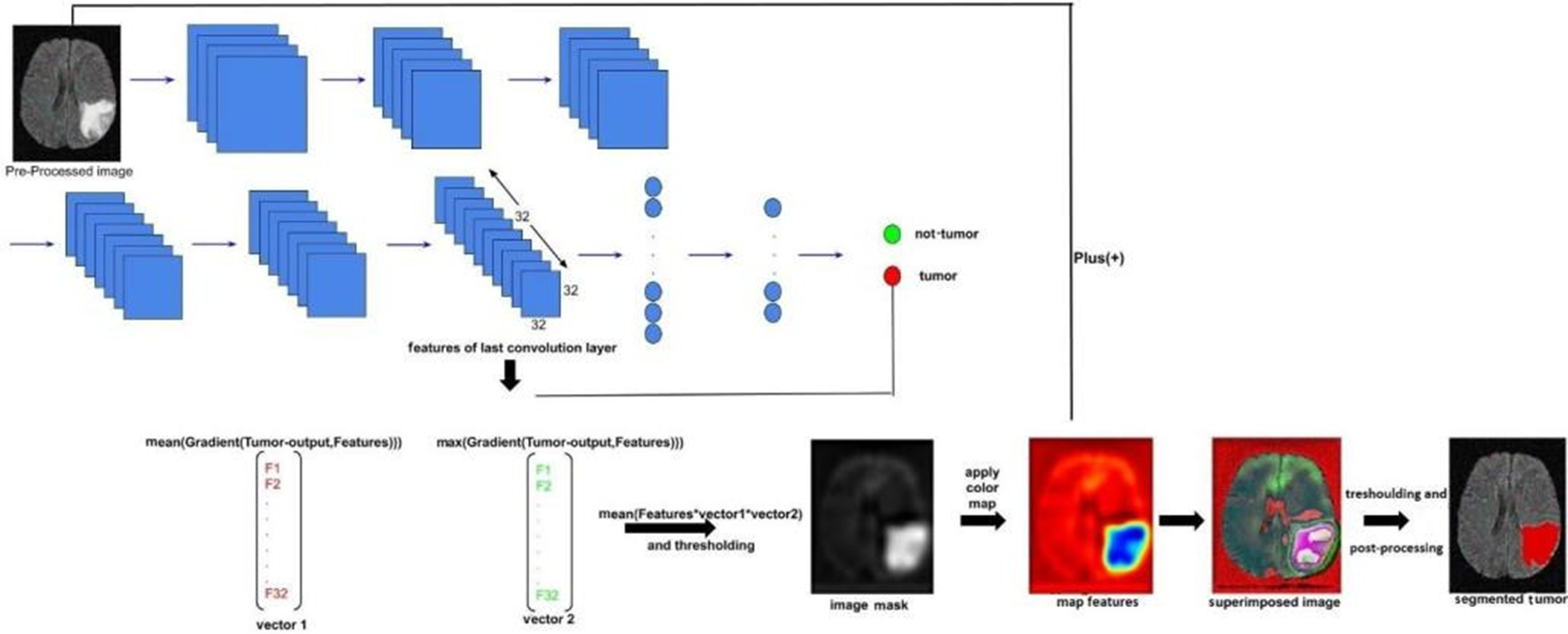
Deep learning software is the ideal choice because it can extract more significant information from the entire picture than is possible to do manually. The majority of deep learning-based segmentation techniques need masked pictures that depict the desired final outcome. These labels undoubtedly aid in directing the learning process in these segmentation tasks.However, the process of producing them still requires a significant amount of time, and another issue is the subjectivity of experts.To address these issues, we developed a CNN-based approach for segmentation that does not rely on masked pictures.We actually made an image by combining the gradient of the last layer of features with the mean and maximum of each image filter extracted from the last layer. This was done after predicting the presence of a tumour using a CNN architecture that we trained without using labels in the form of images but rather as two numbers (0 or 1).


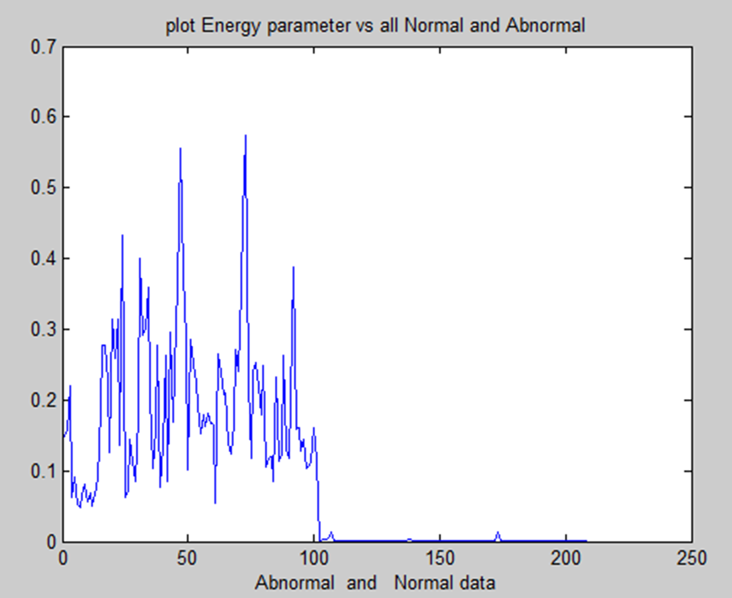
Energy feature of normal and abnormal.

Correlation feature of normal and abnormal.
A convolutional neural network (CNN) is one type of neural network that can extract significant characteristics from pictures, evaluate those features, and categorize them effectively. As a result, CNN outperforms all previous deep learning models in picture classification.The majority of CNN's distinct designs consist of three primary layers: the fully connected layer, the pooling layer, and the convolution layer. Convolutional layers only function at a single point in time. This converts the layer before it into the next layer after separating the differences from the original data.The pooling layer then begins to learn from the previous layer and strives to simplify the process.The fully connected layer finally applies the characteristics gathered from all previous layers to categorize the outputs.
In medical research, combining methods for detecting brain tumors with digital image processing has proved challenging. Finding more effective ways to detect brain tumors is the aim of comparative research. This research provided an overview of the various methods for detecting brain tumours. The picture's inherent geometric measures illustrate how the system relies on forms that change over time. You can see a few items and the inner and outside borders simultaneously since the advancing shapes truly divide and reassemble.The foundation of this approach is the connection between dynamic shapes and the very seamless computation of geodesics or bends. This geodesic technique makes it possible to combine energy-saving conventional “snakes” with geometric forms that move according to the theory of bend development, thereby promoting division. We test the approach using actual images of objects with holes and medical information symbols to demonstrate its power. A straightforward method for segmenting images according to their location is region building. Because it allows you to decide where to begin, it is also known as a pixel-based image division approach. This division method examines the pixels next to the initial “seed focusses” to determine their inclusion in the area. The procedure is conducted in the same manner as computations for general information grouping. A watershed is a region of land with high points and ridges that slope down into lower points and stream valleys. Consider a low-contrast picture as a map, where the dark level of each pixel corresponds to its relief height. When a drop of water falls on a slope, it travels downward until it reaches the lowest point in the area. Naturally, the watershed of an alleviation corresponds to the furthest point of the nearby bowls of water that collect the drops. Picture processing allows for the handling of various watershed lines. Charts can display certain items on the hubs, the edges, or both. The persistent space also allows for the description of watersheds. There are various ways to determine the size of a watershed. We encode the slope size, or the length of the inclination vectors, in height data for division. Artificial neural networks (ANNs), as opposed to conventional model-based approaches, use a self-adaptive strategy that is powered by non- straight information. They are effective instruments for establishing a point, particularly when the connection between the concealed information is unclear.The graphic displays the entropy analysis of normal and atypical brain tumorsis shown in Figure 22. The figure displays the total average analysis of normal and atypical brain tumors is shown in Figure 23. The image illustrates the sumvariance analysis of both normal and atypical brain tumours is shown in Figure 24.
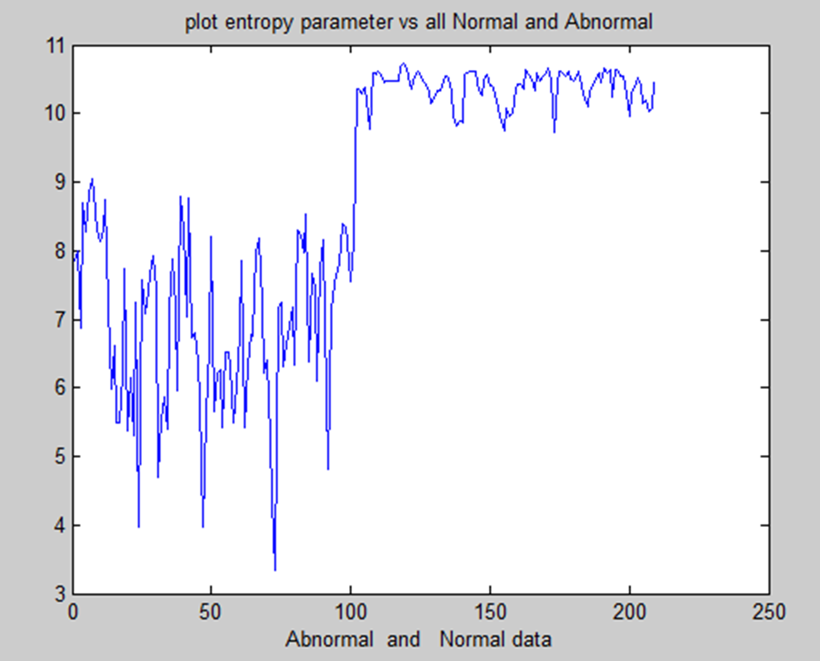
Entropy analysis of normal and abnormal.
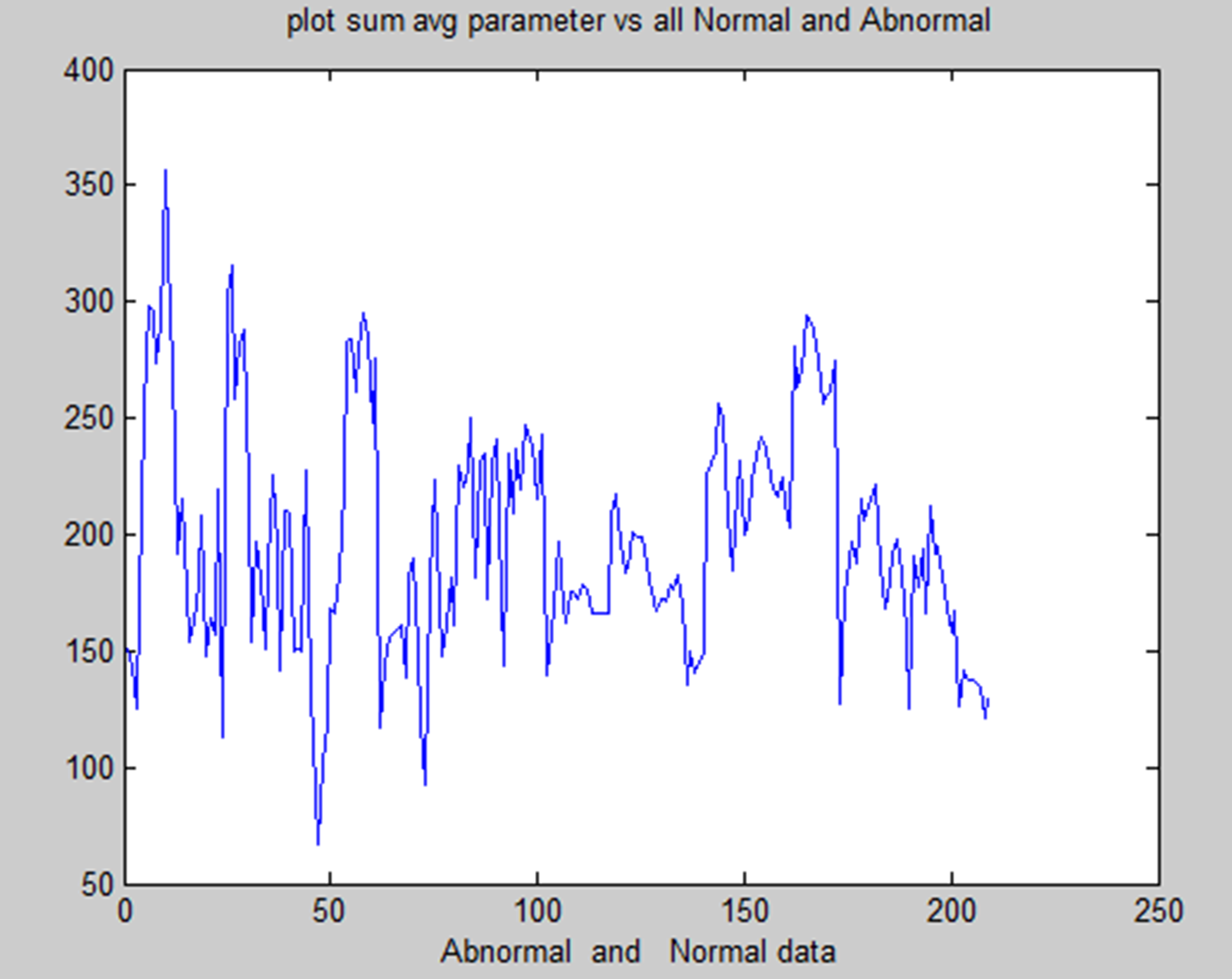
Sum average of normal and abnormal.
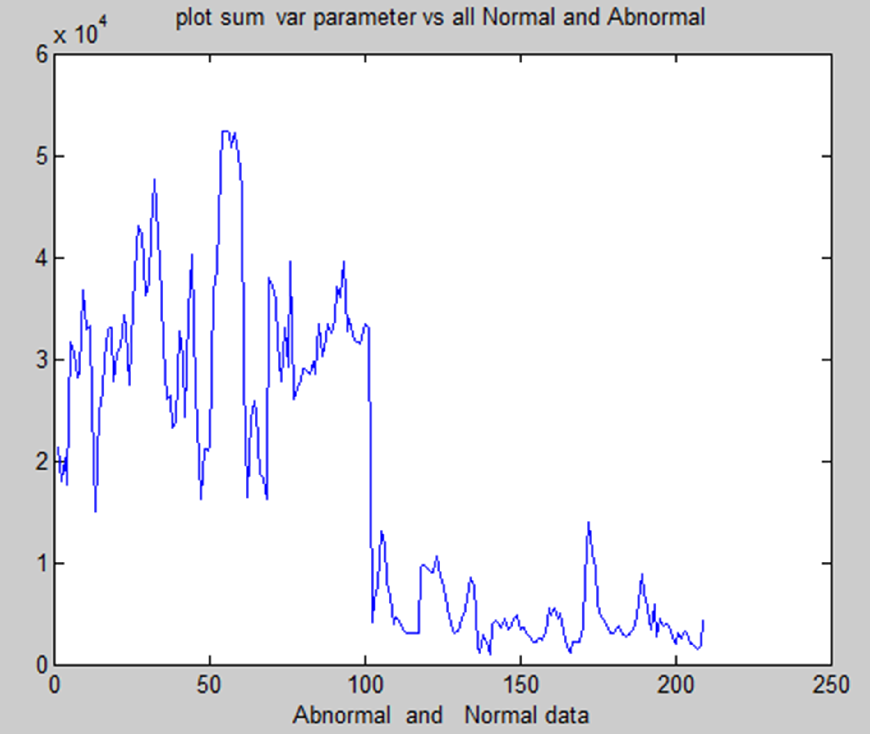
Sum variance of normal and abnormal.
We have used one clustering method and one segmentation method for this. We preprocess every MRI picture to remove noise and then enhance it to provide a crisper image. This paper offers two methods for location.
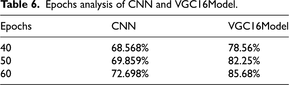
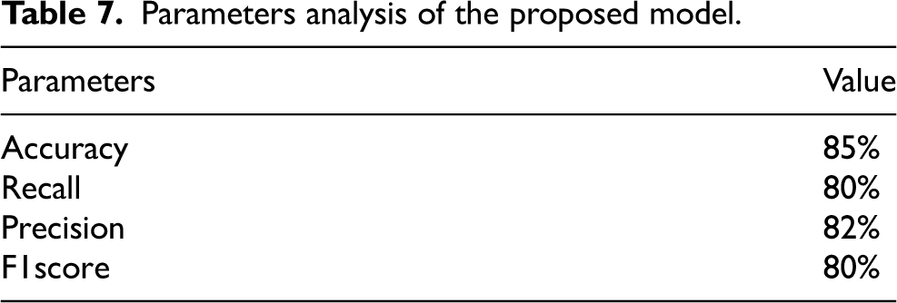
The tumour in a picture is then used. SVM classification and SOM clustering are two examples of these divisions. We can determine which segmentation technique works best for removing the cancer from each picture by using each one. The tumour area consists of the pixel values extracted from a texture picture using the ginput() function for the foreground points. The rangefilter technique creates the texture picture. We apply a smoothing filter to the texture picture to enhance its appearance. Finding and removing the appropriate portion of the photograph that displayed the tumour was the most difficult aspect of this undertaking. Due to lighting issues, the picture contained an excessive amount of white space, potentially misinterpreting it as a tumor. Additionally, the picture incorrectly identifies many areas as tumours due to poor contrast and undesired noise. Other issues during acquisition may have caused the MRI picture quality to be lower than expected. Although there are now many methods for identifying and separating brain cancers from brain pictures obtained with an MRI, our study has shown that it can achieve an average accuracy of up to 97%. We have covered every step involved in brain cancer detection, from obtaining an MRI to classifying the tumour using the two segmentation algorithms. Epchos Anlaysis of CNN and VCG 16 model is shown in Table 6 and Figure 25 provide the CNN and VGC-16 models’ epoch analyses. Parameters analysis of the proposed model is shown in Table 7 and Figure 26 provide the performance analysis of the suggested model.
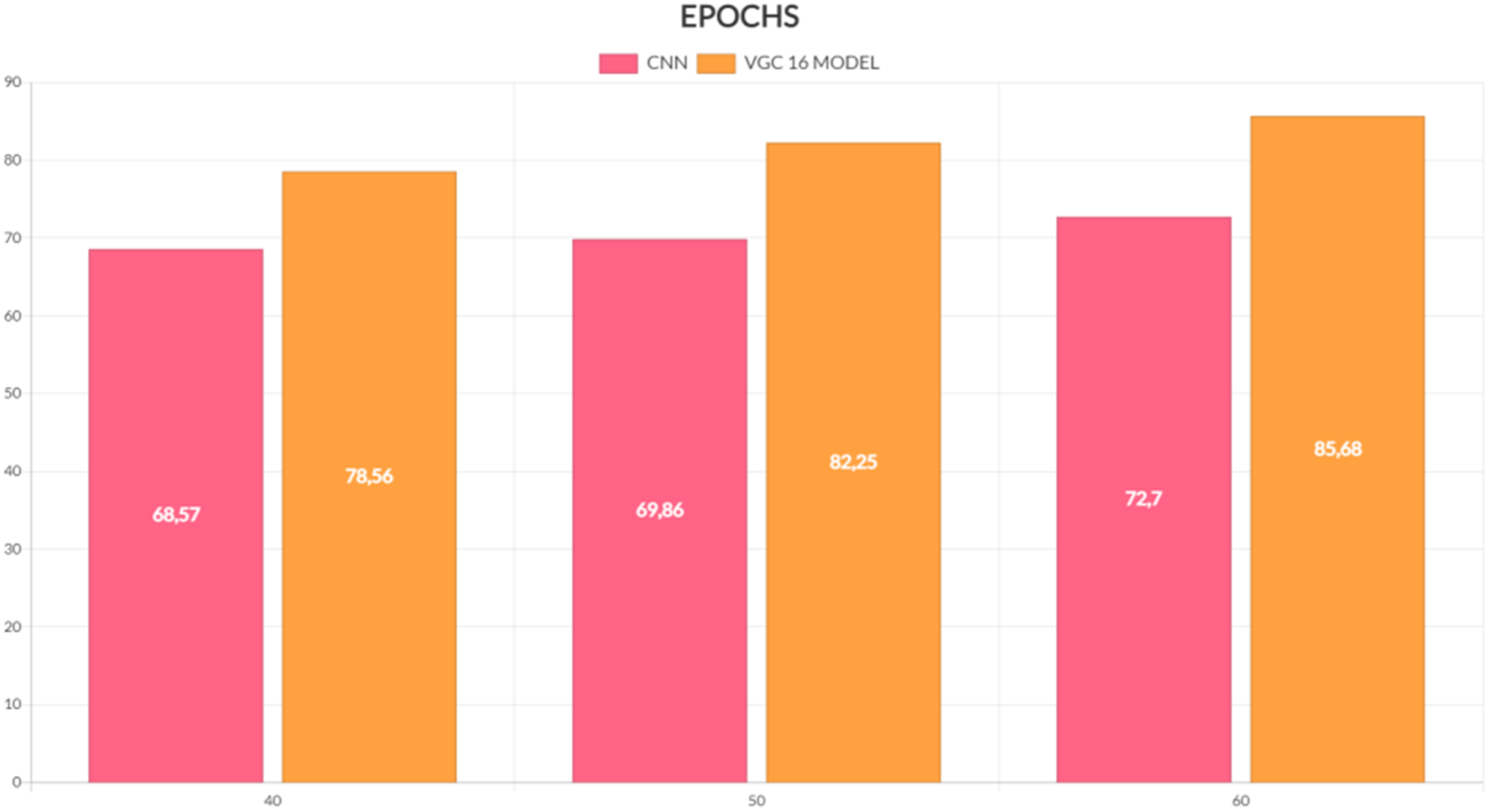
EPOCHS analysis.
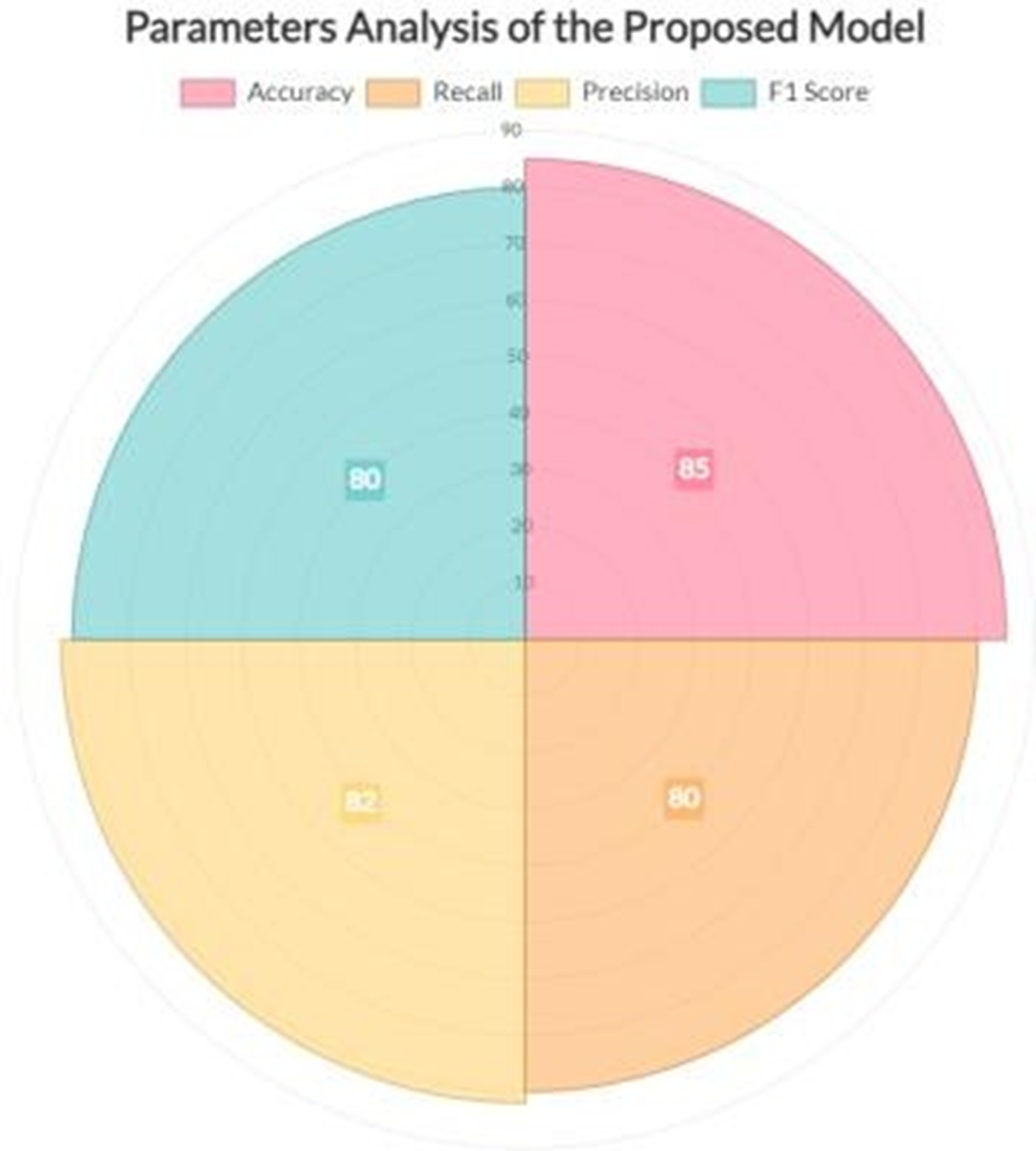
Performance analysis of the model.
Epochs analysis of CNN and VGC16Model.
Parameters analysis of the proposed model.
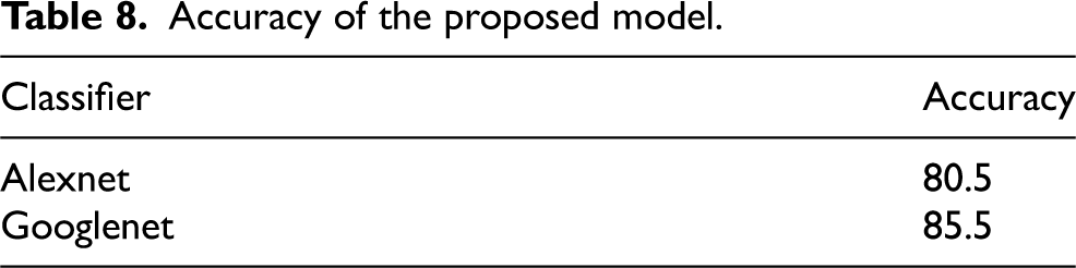
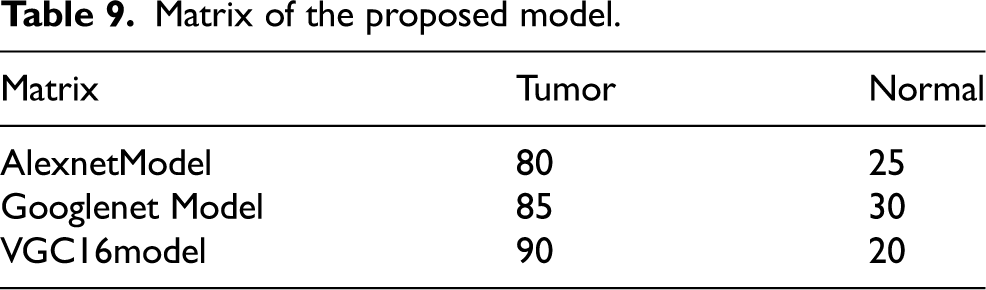
We have discussed preprocessing methods such as wavelet-based techniques. Quality improvement and filtering are crucial because they sharpen edges, make them stand out more, eliminate noise, and remove undesirable backgrounds. Out of all the filtering techniques, the Gaussian filter proves to be the most effective in identifying outliers without compromising the sharpness of the pictures, and in removing noise without obscuring the edges. It processes more quickly than other filtering techniques, reduces noise, and improves the quality of the pictures. We used a technique to separate a brain tumour from a brain MRI after improving picture quality and reducing noise. For large datasets, classification-based segmentation may reliably separate tumors and provide insightful findings. However, failure to include a category in the training data might have negative consequences. For noise-free pictures, cluster-based segmentation is simple, fast, and produces excellent results. However, the segmentation becomes much less accurate when the picture contains noise. One of the main issues with neural network-based segmentation is the learning process, although it performs better in noisy situations and does not need assumptions about the distribution of data. Although there were issues, they were resolved, and reliable results for brain cancer detection were obtained by automating the segmentation of brain tumours using a mix of threshold-based and classification using SVM and SOM. These classification techniques can first determine if a tumor is present and, if so, whether it is benign or malignant is shown in Figure 28. Table 8 and Figure 27 provide the accuracy analysis of the suggested model. Table 9 and Figure 28 provide the matrix analysis of the suggested model.
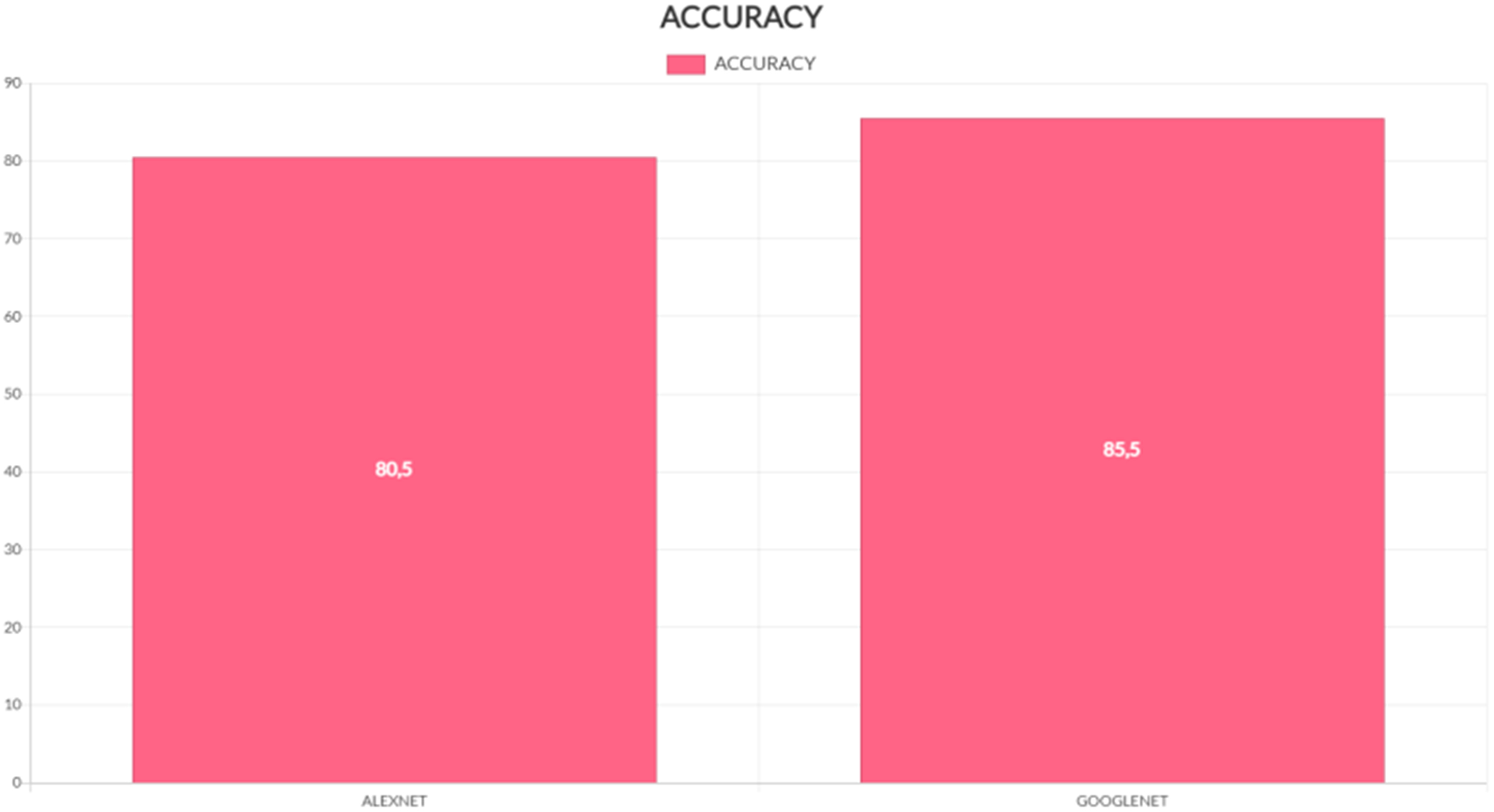
Accuracy analysis of the model.
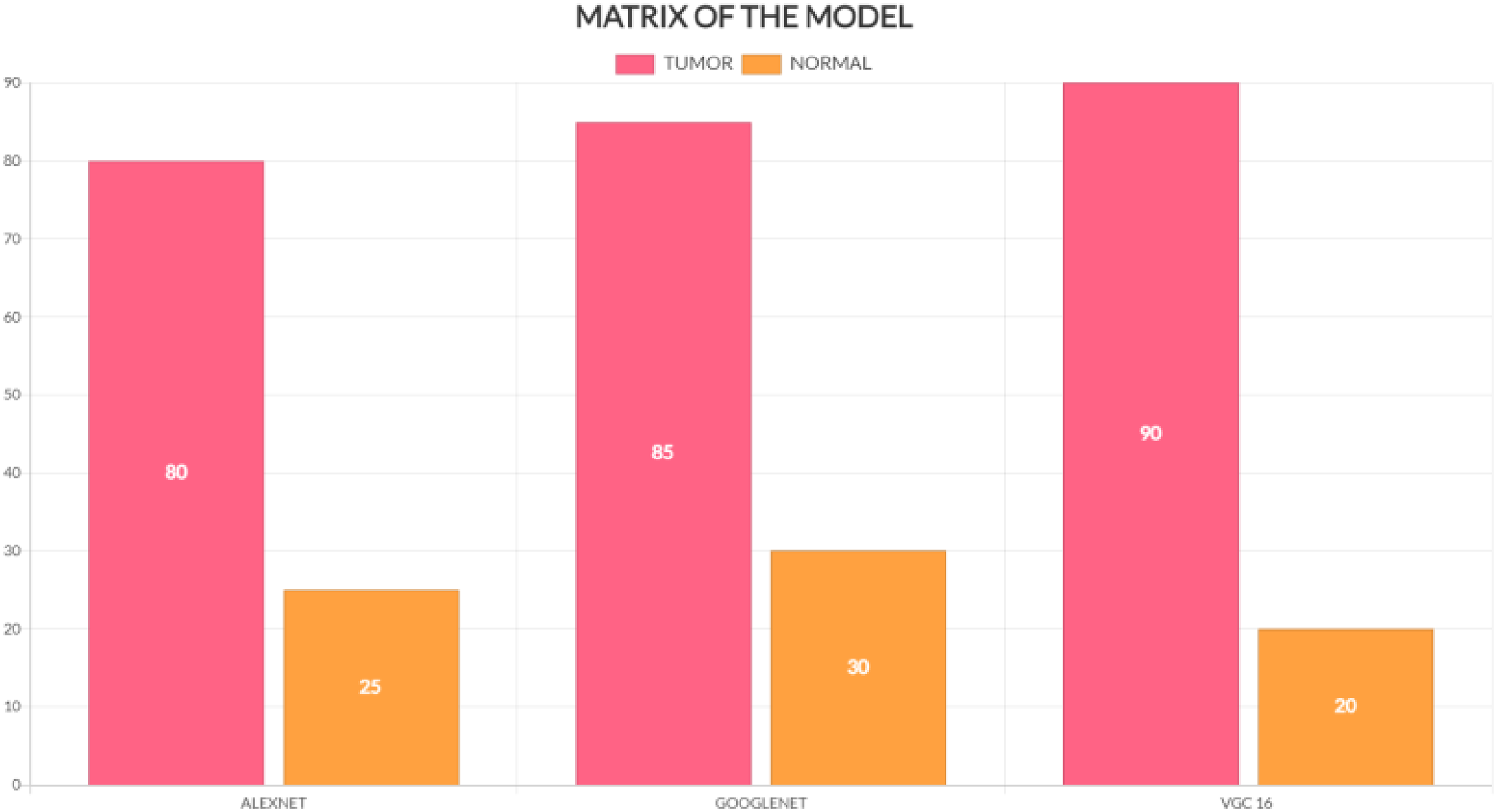
Matrix analysis of the model.
Accuracy of the proposed model.
Matrix of the proposed model.
Good machine learning models rely on having a lot of high-quality data. However, it might be difficult to get adequate data, which can slow down the creation of a model. You may add to your dataset to compensate for a shortage of data. Clever programming techniques can expand your training set by adding data. Even better, an improved training set often leads to a more stable and potentially simpler model. Here, we rotated each picture in the training set 300 degrees to the left and 300 degrees to the right after flipping it horizontally.This gave us the opportunity to work with a variety of data.People consider brain tumors one of the world's most deadly causes of death. Therefore, it is crucial to discover brain tumours as quickly as possible. There are numerous theories regarding how to predict andsplit the controversy. However, they face a number of issues, such as the need for expert assistance, a lengthy operation, and difficulty in selecting an appropriate feature extractor. We developed a technique based on the design of a convolutional neural network that seeks to simultaneously forecast and split a rebral tunnel in order to address these issues. We divided the plan into two sections. Firstly, we implemented a straightforward binary annotation to determine the presence of cancer, eliminating the need for tagged photos, which necessitates expert assistance. We obtained the final categorisation by feeding the prepared picture data into our deep learning model. We used the feature representations created by the convolutional neural network designs to filter out any classifications that indicated the presence of a brain tumour. We trained the suggested approach using various types of gliomas from the BraTS2017 dataset. The findings demonstrate the effectiveness of the suggested approach in terms of recall, accuracy, precision, and the Dice similarity coefficient. Our approach achieved a 92% classification accuracy for cancers and an 83.35% Dice similarity coefficient for tumour division.
Conclusion
The integration of machine learning techniques, particularly deep learning methods like CNNs, with medical imaging modalities like MRI and CT has greatly advanced the field of medical image analysis. These techniques enable the automatic detection and classification of abnormalities like brain tumors, offering great potential for improving diagnosis and treatment planning. However, challenges remain, particularly in segmentation, handling noisy or low-quality images, and managing the high computational demands of 3D medical imaging. Ongoing research is focused on improving these models, reducing computational complexity, and increasing accuracy in medical image classification tasks. By continuing to refine these techniques and incorporate more diverse data sources, the potential for machine learning to aid in the detection of medical conditions like brain tumors will only grow, ultimately leading to more efficient and accurate medical diagnoses. In conclusion, the combination of advanced imaging techniques and machine learning algorithms like CNNs has drastically transformed medical image processing, especially in tumor detection and brain imaging. These technologies have allowed for more accurate and efficient diagnosis, leading to better patient outcomes. As research continues to advance, the integration of AI and machine learning into medical imaging holds great promise for revolutionizing healthcare, offering new possibilities for early detection, personalized treatment plans, and improved patient care. The ongoing efforts to refine and enhance these technologies will continue to shape the future of medical diagnostics and therapeutic interventions.This research demonstrates the effectiveness of using CNNs for tumor detection in MRI slices, with both GoogLeNet and AlexNet showing promising results. The proposed system achieved an accuracy rate of
Future work could involve expanding the dataset to include more diverse MRI slices, exploring additional CNN architectures, and integrating this system into real-world clinical workflows for more extensive evaluation.
Footnotes
Author contribution
Shunmugavel Kannadhasan – Design, Implementation, Conceptualization, Analysis of Data, Writing, Editing, Revision and Results. Ramalingam Gomathi – Design, Implementation, Conceptualization, Analysis of Data, Writing, Editing, Supervision, Revision and Results. Suriyan Ganesh – Design, Implementation, Conceptualization, Analysis of Data, Writing, Editing, Revision and Results.
Funding
The authors received no financial support for the research, authorship, and/or publication of this article.
Declaration of conflicting interests
The authors declared no potential conflicts of interest with respect to the research, authorship, and/or publication of this article.