Sage Journals: Discover world-class research

Abstract

Spanish

In this paper, I use a slightly modified version of the Becker–Stigler model of corrupt behavior to explain bureaucratic political involvement. Since bureaucrats prefer higher rewards and not to support losing candidates, we expect them to become politically involved near elections – when rewards are expected to be higher, and information more abundant. Taking advantage of a natural experiment, I employ differences-in-means and differences-in-differences techniques to estimate the effect of electoral proximity on the political involvement of justices of the peace in the city of Buenos Aires in 1904. I find a large, positive, and highly local effect of electoral proximity on their political involvement, with no appreciable impact in the months before or after elections.

Keywords

Argentina bureaucracy electoral fraud burocracia fraude electoral

Introduction

In competitive settings, politicians often engage in clandestine and illegal efforts to shape electoral results (Lehoucq 2003). Electoral fraud can take many forms, including vote and turnout buying, ballot stuffing, vote miscount, and violent intimidation. Recent research on the topic has shown that the execution of electoral fraud typically requires operational support from brokers and bureaucrats at the local level (Cantu 2014; Benton 2013; Larreguy, Olea, and Querubin 2014; Martinez-Bravo 2014; Simpser 2013; Svolik and Rundlett 2014).

Because of a revived interest in the study of the execution of electoral fraud, the growing literature on the political involvement of public officials has focused exclusively on their illegal activities during elections, but not the moments before or after them. However, the execution of electoral fraud is, at a more general level, only one specific task undertaken by politically involved bureaucrats who also agree to perform other (often complementary) duties, such as attending political meetings, persuading others, and providing information to the candidates they support (Zarazaga 2014).

Bureaucrats are mainly motivated by career concerns and prospects for future employment (Alesina and Tabellini 2007). For this reason, for example, elected judges in democratic regimes become more punitive when elections are on the horizon (Huber and Gordon 2004), even more so when they face serious competition (Gordon and Huber 2007). Appointed public employees, on the other hand, have strong incentives to support popular candidates because their positions or promotions will be decided by the incoming government (Martinez-Bravo 2014).

In competitive authoritarianisms, Way (2006) noted that it is unlikely that bureaucrats will support candidates who they suspect will lose the election, since this might offend the winning candidate. In these settings, bureaucrats have to decide before elections whether to get politically involved. If they choose wrong – that is, if they support a losing candidate – then they will likely lose their office. If they choose the winning candidate, they will be rewarded – compensations may include anything from relationships with incumbents to higher office.

Electoral fraud, specifically, takes place on the day of the election or during the vote count, but when are bureaucracies politicized? When do bureaucrats decide to surrender technocratic duties to join a network of political operatives that, after agreements and planning, eventually ends up executing electoral fraud on the ground? Do bureaucrats stay constantly involved in politics or does this involvement vary over time? Building on the Becker–Stigler model of agent corruption (1974), I argue that bureaucrats decide to get involved in political activities when rewards are high and electoral information abundant. Therefore, the political involvement of bureaucrats should be expected to grow as elections approach and to remain low both before then and afterwards.

I test this prediction using a quasi-experimental research design. ¹ In 1904 the newly enacted Argentine electoral law mandated that elections for the partial renewal of the House of Representatives should be held in only half of the country's electoral districts, selected by a public lottery in Congress. This lottery has provided random variation in electoral timing, which can be used to estimate its effect on the political involvement of bureaucrats.

1
On the respective advantages of experimental research and observational research, see Gerber, Green, and Kaplan (2004) and Morton and Williams (2010). On natural experiments, see Dunning (2012).

Taking advantage of the opportunity provided by this natural experiment, I estimate the effect of electoral proximity on the political involvement of justices of the peace in the city of Buenos Aires using differences-in-means and differences-in-differences techniques. I assume that the performance of bureaucrats diminishes when their political involvement increases because of competition between political and technical activities for that bureaucrat's time. Using monthly data on civil marriages as an “effect indicator,” I show that electoral proximity has a strong, positive, and highly local effect on bureaucratic political involvement, with no appreciable impact in the months before or after elections.

As an empirical contribution, this paper isolates the effect of electoral proximity on bureaucratic political involvement. Theoretically, the conclusions of this paper contribute to three different areas of research. First, by allowing intertemporal variation in bureaucratic active support to incumbents, they complement research on electoral competition in authoritarian regimes by introducing a possible explanation for the fact that incumbent candidates can lose elections, even in competitive regimes with strong bureaucratic political machines (Brownlee 2007; Gehlbach and Keefer 2008; Magaloni 2008; Lazarev 2005; Magaloni and Kricheli 2010). Second, the conclusions extend arguments about the effect of career concerns on bureaucratic behavior – mostly developed for democratic regimes – to autocratic institutional settings (Martinez-Bravo 2014; Huber and Gordon 2004; Gordon and Huber 2007; Ahuja 1994; Elling 1982; Wright and Berkman 1986; Croley 1995). Third, they further gauge the causal dynamic of the autocratic search for popularity (Wintrobe 1998; Gehlbach and Simpser 2013; Kuran 1995).

1 Theory

I consider bureaucrats politically involved when they participate in partisan activities with the intention to shape the political sphere or to influence electoral outcomes. Political involvement increases 1) when uninvolved bureaucrats decide to take part in partisan affairs and 2) when already-involved bureaucrats augment their level of political participation. Disentangling these two situations would require the establishment of a specific minimum threshold of political involvement, above which bureaucrats are said to be politically involved. That conceptual enterprise is beyond the scope of this paper. In what follows, I refer broadly to political involvement as encompassing both alternative situations.

In this paper, I use a slightly modified version of the Becker–Stigler model of corrupt behavior (1974) to explain the political involvement of bureaucrats in competitive regimes. This simple model considers the choice that must be made by a bureaucrat with the opportunity to get involved in politics.

Before a given election, a bureaucrat has to decide whether and how much to get involved in political issues in support of a given candidate. Supporting a candidate frequently entails executing electoral fraud, but it is not limited to this single activity. Politically involved bureaucrats also attend partisan meetings, persuade potential voters and other bureaucrats, inform candidates about the political alliances and voter mobilization plans of their political rivals, ² and design the operational tasks for vote or turnout buying on the day of the election.

2
In a recent paper, Zarazaga (2014) has shown that political operatives at the local level are valuable sources of information for their principals.

If a bureaucrat decides not to get involved in politics, he is guaranteed his wage, w. If he chooses political involvement, he has to play a lottery: there is some probability (1-θ) the candidate he supports will win the election, and that the bureaucrat will get his wage and r, a reward. Rewards may include anything the candidate can credibly offer (relationships, money, land, a promotion, political office, among many other things). Assuming that a bureaucrat who supports a losing candidate is fired by the newly elected government, the punishment depends on the wage he would earn in other employments, w^o. The key equation in this model can be written as follows (Di Tella and Schargrodsky 2003): a rational bureaucrat prefers political involvement when

θ (w - w^{0}) < (1 - θ) r .

(1)

The simple model presented above could explain why bureaucrats who are not constantly involved in politics might agree to support a given candidate during elections. The time-dependent nature of bureaucratic political involvement can also account for the fact that incumbents with strong state-owned political machines can be defeated in elections, like the autocrats from Slovakia (1998), Croatia (2000), Serbia (2000), Georgia (2003), Ukraine (2004), and Kyrgyzstan (2005) during the “color revolutions” (Bunce and Wolchik 2011).

The model predicts that, everything else held equal, the political involvement of bureaucrats will increase in three alternative scenarios: (1) when the difference between their wage and their expected wage in the alternative employments decreases, (2) when promised rewards increase, and (3) when certainty about future electoral results increases.

Opportunities for alternative employment are expected to depend on the experience, education, and ability of individual bureaucrats. Rewards and certainty about future electoral results, however, should be expected to increase near elections by way of two mechanisms, everything else held equal. First, as the day of a given election arrives, bureaucrats have access to better information regarding the political alliances and electoral competitiveness of each individual candidate. This information allows them to choose which candidate to support, based on their expected probability of electoral success. The penalty for supporting losing candidates is twofold: For one thing, bureaucrats offend winning candidates and risk losing their jobs. In addition, the candidates they supported are not able to deliver on their promises because they could not access political office.

Second, as the need for bureaucratic political involvement becomes more salient, candidates should be more willing to offer higher rewards near elections. As noted by Gehlbach and Simpser (2013), candidates might also increase the magnitude of rewards to create a perception of popularity among other bureaucrats, in order to ensure further support.

If this theory explains bureaucratic political involvement, then bureaucrats should be more likely to choose political involvement near elections, when rewards and certainty are expected to be higher. I test this observational implication below by exploiting a natural experiment in Argentina in 1904.

2 Bureaucracy and Politics in Argentina (1880–1912)

In his groundbreaking book, historian Natalio Botana described nineteenth-century Argentina's political system as an “inverted representative system.” In the absence of a secret ballot, public officials acted as electors within a “network of political control” ³ (Botana 1985: 184) and engineered elections in which incumbent candidates almost invariably succeeded. Fraud was guaranteed by bribes, distribution of public employment and, overall, the mutual dependency between the bureaucratic structure and the political system (Castro 2004; Gomez 2013). Secret personal arrangements (Alonso 2010) and family ties (Losada 2012) established the rhythm of everyday politics.

3
Unless otherwise noted, all translations into English are my own.

On the day of elections, the winning faction was the one that had the best-organized political machine and managed to show up at the polls with the greatest number of voters (Sabato 2004). In 1904 an observer noted that vote buying was practiced with the complicity of public authorities and in public: outside hospitals and schools, in churches, and next to voting tables (Zeballos 1904). Voters were paid in cash, and taken from political committees to the polls in partisan cars (Botana 1985: 304). Given that voting was public (and not secret), vote counts were instantaneous. Therefore, when results were close, political operatives would go to the streets and buy votes on the spot (Jorrat and Canton 1999).

Vote buying was practiced by all political factions (Sabato 2004; Zimmermann 2009), and it was executed at the local level by a network of judges, policemen, and members of the National Guard, without logistical support from landowning elites (Halperín Donghi 1992, 2007; Castro 2004; Hora 2001). In this setting, the judiciary was frequently used as an intermediate step to higher political positions, and previous political activities were seriously considered at the time of candidate selection (Zimmermann 1996). ⁴ The judicial and political spheres were intimately linked (Zimmermann 2007). ⁵

For a discussion of the importance of political ties and electoral support for the appointment of judges, see Zeballos (1902).

Using an arbitrary sample of 60 federal justices, Zimmermann (2007) shows that they all occupied political positions before or after their judicial appointments.

The typical career path of justices went something like this: After graduating in law, lawyers received minor political offices or a judicial position at the provincial level. They then became federal justices, and this allowed them to climb to higher provincial and national positions. Former justices later became national ministers, federal interventors, national senators, or national members of Congress (Zimmermann 1996). Most of their political capital was developed during their mandates as local justices, when they performed an important role as political brokers. According to Representative Estanislao Zeballos, justices of the peace were “the key to electoral success” (Diario de Sesiones de la Cámara de Diputados 1882, I: 123).

The organization of bureaucratic political machines required the construction of political alliances before elections. Representative Pastor Lacasa argued that the success of Vice President Pellegrini's party in the 1906 House election was not due to the quality of its candidates, but because Pellegrini “went to political committees, worked night and day, and he himself went to the houses of important men to ask for their support” (Diario de Sesiones de la Cámara de Diputados 1911, I: 291). When building electoral coalitions for upcoming elections, candidates would write to justices. Running for governor of Santiago del Estero, Pedro Gallo sent letters to all judges in the province, telling them that “a party list had been written in a meeting with many friends” and that they should “support it and make it succeed.” ⁶

Francisco Olivera to Julio A. Roca, Santiago del Estero, 1 August 1882 (AGN, Argentina, Sala VII, Archivo Roca, Leg. 21).

Given that the control of the state apparatus was not, by itself, enough to win elections, candidates depended on “clubs” for voter mobilization. These grass-roots organizations were constructed on existent social relations, rendering justices of the peace their natural leaders, as their social position as notables gave them a comparative advantage in supporter recruitment. Once candidacies were defined, political clubs publicly promoted candidates and supervised electoral operations – these included identifying supporters and registering them to vote, persuading potential voters, and organizing partisan meetings and rallies (Sábato 2004).

Considering that electoral winners were likely to reward supporters and punish others, it was not always easy to decide whether to support a given candidate. Even governors were reluctant to support any presidential candidate long before the 1904 election (Castro 2004). According to an article in the daily El Diario, by 9 September 1903 candidates competing in every district were already defined and establishing their political committees (quoted in Cantón and Jorrat 2004: 343–348). The time to build electoral support had started. As an example, industrialists were said to already be supporting Eliseo Cantón in San Cristobal Sud, and the president's secretary, Jaime Llavallol, endorsed Benjamín González as a candidate in San Juan Evangelista, with the support of the chief of police, Agustín Mascias. By September 1903, however, it was still unknown how 600 votes from municipal employees in San Cristobal Norte would be cast (Cantón and Jorrat 2004: 344).

Once candidates were elected, and in the absence of a meritocratic bureaucracy, they enjoyed the freedom to appoint or favor political friends (Sábato 2004). This power was frequently used to build up new political machines or reward allies from past electoral struggles. Castro quotes a letter from a judge to President Julio Roca in 1902 that is illustrative of this point:

My Dear Julio, […] today, I ask […] that […] when there is a vacancy, you put me in the Supreme Court […]. Almost all of my colleagues from that time […] are there […]. I did not go because I served as a bumper as president of the Civil Chamber in that famous election you surely have not forgotten. (Castro 2004: 24)

When personal ties or career dependence were not enough, judges were directly bribed. When running for president, Juárez Celman received a letter from the governor of Catamarca, who was concerned because rochistas (the opposition) had sent emissaries all over the province in order to “corrupt judges with bribes.” ⁷ In that same presidential election, the incumbent party of the province of Jujuy was weakened because of the magnitude of rochista bribes, and the governor wrote President Julio A. Roca (Juárez Celman's brother-in-law) to remind him that their party “would only be able to win the upcoming election with help from the judiciary.” ⁸

José S. Daza to Juárez Celman, Catamarca, 11 January 1886 (AGN, Argentina, Sala VII, Archivo Juárez Celman, Leg. 20).

J. M. Álvarez to J. A. Roca, Jujuy, 2 December 1886 (AGN, Argentina, Sala VII, Archivo Roca, Leg. 50).

If justices did not support winning candidates, they could be removed from their positions. Federal Justice Romero recommended that Governor Rocha “remove opposing justices” and “make them understand that they are […] subject to their political bosses, whose orders they are obliged to obey.” ⁹

José Benjamín Romero to Dardo Rocha, Corrientes, 18 June 1878 (AGN, Sala VII, Archivo Rocha, Leg. 217).

3 Research Design and Data

In 1902 the National Congress approved a new electoral law, proposed by Minister of Interior Joaquín V. González, with support from President Roca. This law – no. 4161 – mandated that elections for the House of Representatives be held in 120 single-member districts, replacing provinces as multimember districts. Historiographical accounts attribute the electoral reform exclusively to Minister González (Pereyra 1999; de Privitellio 2006). In fact, the reform did not change the electoral landscape, and was suppressed in 1905 by President Manuel Quintana during his first year in office.

The law was made operative by a presidential decree in March 1903. ¹⁰ It ruled that the country be divided into 120 single-member districts, and it set the limits of districts in the city of Buenos Aires, while delegating the division of provinces to local legislatures. Districts were to be assigned according to the population data from the National Census of 1895, and they were required to have a population that allowed the election of exactly one representative. In cities, article 28 requested that districts coincide with parochial divisions.

10
Boletín Oficial de la República Argentina, Año XII, No. 3078, 12 January 1904.

Given that, by constitutional law, only half of the seats in the House of Representatives were to be contested in 1904, article 22 of the presidential decree ordered that a public lottery take place in Congress to choose which single-member districts in each province would compete in the first election. ¹¹ This lottery provided random variation in elections among districts.

The undisputed results of the public lottery were sent to President Roca by Representative Benito Villanueva and Secretary Alejandro Sorondo on 1 June 1903 (see Boletín Oficial de la República Argentina, Año XI, No. 2951, 8 August 1903: 1).

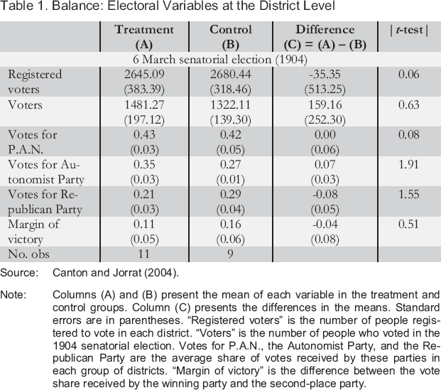
In this paper, I use this exogenous assignment of elections to estimate their effect on the political involvement of justices of the peace (JOPs) in the city of Buenos Aires. ¹² The city was divided into 20 singlemember districts, and elections were held only in 11 of them (the treatment group) in March 1904. The other nine districts represent the control group. Simple t-tests in Table 1 show that the two groups were balanced in terms of pre-treatment characteristics, using data on the electoral results of the senatorial election of 1904. I interpret the similarity in these variables as informative of the similarity between groups in other variables, both observable and unobservable.

Of course, considering only this city is arbitrary. Nevertheless, Buenos Aires is the only district with a developed system of public statistics. The next national census, a possible source of data for other provinces, was published in 1914: ten years after the election. Furthermore, the boundaries of districts in the other provinces, unlike those of the city of Buenos Aires, are not specified in presidential decrees. However, historians agree that the political involvement of JOPs was most important in rural areas (Cárcano 1986; Hora 2001; Lopez 2005). Consequently, finding a significant effect in the fully urbanized city of Buenos Aires – the place where effects are least likely to be seen – suggests a higher impact in other provinces (Gerring 2007). Levy (2008: 12) describes this logic as the Sinatra inference: “If I can make it here, I can make it anywhere.”

Table 1

Balance: Electoral Variables at the District Level

	Treatment (A)	Control (B)	Difference (C) = (A) – (B)	\|t -test\|
6 March senatorial election (1904)
Registered voters	2645.09 (383.39)	2680.44 (318.46)	-35.35 (513.25)	0.06
Voters	1481.27 (197.12)	1322.11 (139.30)	159.16 (252.30)	0.63
Votes for P.A.N.	0.43 (0.03)	0.42 (0.05)	0.00 (0.06)	0.08
Votes for Autonomist Party	0.35 (0.03)	0.27 (0.01)	0.07 (0.03)	1.91
Votes for Republican Party	0.21 (0.03)	0.29 (0.04)	-0.08 (0.05)	1.55
Margin of victory	0.11 (0.05)	0.16 (0.06)	-0.04 (0.08)	0.51
No. obs	11	9

Source: Canton and Jorrat (2004).

Note: Columns (A) and (B) present the mean of each variable in the treatment and control groups. Column (C) presents the differences in the means. Standard errors are in parentheses. “Registered voters” is the number of people registered to vote in each district. “Voters” is the number of people who voted in the 1904 senatorial election. Votes for P.A.N., the Autonomist Party, and the Republican Party are the average share of votes received by these parties in each group of districts. “Margin of victory” is the difference between the vote share received by the winning party and the second-place party.

4 Dependent Variable: Bureaucratic Political Involvement

A central task in the identification of the effect of electoral proximity on bureaucratic political involvement is the measurement of the latter. This is particularly challenging, considering that this variable is not directly measurable.

Since the enactment of the Civil Marriage Law (no. 2393) in 1888, JOPs were in charge of officiating civil marriages. Therefore, I use the number of civil marriages per 1,000 registered voters in each district as an “effect indicator” (Bollen and Lennox 1991) of their political involvement. The validity of this indicator rests on the assumption that their performance as public employees and the time they devote to political activities are inversely correlated, because of competition between these two different tasks for time allocation. The hypothetic logic for this inverse correlation is straightforward: political involvement demands attending meetings and political events outside their workplace, where marriages are conducted.

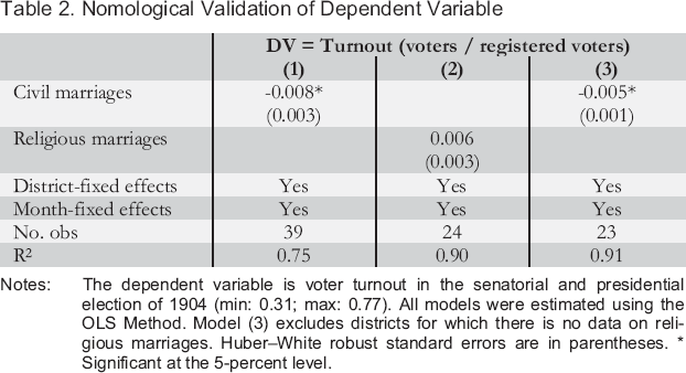
To empirically assess the validity of this effect indicator, I estimated a linear regression of voter turnout and the monthly marriage rate in each district, using data from the senatorial and presidential electoral months of 1904. Given that the political involvement of bureaucrats leads to increased voter turnout (Nichter 2008), this procedure constitutes a construct/nomological validation of the selected indicator (Adcock and Collier 2001: 543). ¹³ Results are presented below, in Table 2.

Table 2
Nomological Validation of Dependent Variable

DV = Turnout (voters / registered voters)

(1) (2) (3)

Civil marriages -0.008^* (0.003) -0.005^* (0.001)

Religious marriages 0.006 (0.003)

District-fixed effects Yes Yes Yes

Month-fixed effects Yes Yes Yes

No. obs 39 24 23

R² 0.75 0.90 0.91

	DV = Turnout (voters / registered voters)
Civil marriages	-0.008^* (0.003)		-0.005^* (0.001)
Religious marriages		0.006 (0.003)
District-fixed effects	Yes	Yes	Yes
Month-fixed effects	Yes	Yes	Yes
No. obs	39	24	23
R²	0.75	0.90	0.91

Notes: The dependent variable is voter turnout in the senatorial and presidential election of 1904 (min: 0.31; max: 0.77). All models were estimated using the OLS Method. Model (3) excludes districts for which there is no data on religious marriages. Huber–White robust standard errors are in parentheses.

Significant at the 5-percent level.

I consider “turnout” a preferable indicator over the vote share of any specific political party because electoral mobilization was practiced by all political factions (Sabato 2004; Zimmermann 2009).

Controlling for both district and month-fixed effects, civil marriages are negatively correlated to voter turnout, as expected. It could be argued, however, that turnout is negatively correlated to marriage rates for reasons that are orthogonal to judicial political involvement. Turnout, for example, might be a consequence of citizens’ political involvement. To deal with this issue, as a placebo test, I estimated the same model but used religious marriage rates as an independent variable. The rate of marriages celebrated by the Catholic Church is not significantly correlated to voter turnout, and the estimated coefficient is positive. In Model 3, I excluded observations for which there is no available data for religious marriages. The correlation remains negative and statistically significant at the 5-percent level. These results suggest that the civil marriage rate is a valid indicator of the political involvement of JOPs.

5 Results

In this section, I estimate the effect of electoral proximity on bureaucratic political involvement. Given the pre-treatment similarities among treatment and control groups in electoral variables, it is worth considering a simple cross-section estimator (Di Tella and Schargrodsky 2004). I therefore present differences-in-means between experimental groups for every month of the year 1904. I expect bureaucrats to get politically involved near elections, because of increased rewards and certainty on future electoral results.

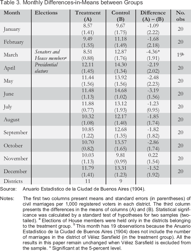
Table 3 presents means (and standard errors) of the indicator of political involvement – the monthly number of civil marriages per 1,000 registered voters – in each group of districts. The third column presents the differences-in-means between the treatment and control groups for every month, and their statistical significance, calculated by a simple (two-tailed) t-test.

Table 3
Monthly Differences-in-Means between Groups

Month Elections Treatment (A) Control (B) Difference (A) – (B) No. obs

January 8.57 (1.41) 9.67 (1.75) -1.09 (2.22) 20

February 9.49 (1.55) 11.18 (1.49) -1.68 (2.18) 20

March Senators and House members^a 8.51 (0.88) 12.87 (1.76) -4.36^* (1.91) 19^b

April Presidential electors 12.11 (1.45) 14.30 (1.34) -2.19 (2.02) 20

May 11.44 (1.56) 13.92 (1.56) -2.48 (2.23) 20

June 11.48 (1.13) 14.68 (1.02) -3.19 (1.56) 20

July 11.88 (0.77) 13.12 (1.93) -1.23 (0.95) 20

August 10.32 (1.08) 12.17 (1.40) -1.85 (1.74) 20

September 10.85 (1.22) 12.68 (1.35) -1.82 (1.82) 20

October 10.70 (0.82) 13.57 (1.65) -2.86 (1.74) 20

November 10.03 (1.13) 9.81 (0.99) 0.22 (1.54) 20

December 11.79 (1.41) 13.31 (1.23) -1.52 (1.92) 20

Districts 11 9

Month	Elections	Treatment (A)	Control (B)	Difference (A) – (B)	No. obs
January		8.57 (1.41)	9.67 (1.75)	-1.09 (2.22)	20
February		9.49 (1.55)	11.18 (1.49)	-1.68 (2.18)	20
March	Senators and House members^a	8.51 (0.88)	12.87 (1.76)	-4.36^* (1.91)	19^b
April	Presidential electors	12.11 (1.45)	14.30 (1.34)	-2.19 (2.02)	20
May		11.44 (1.56)	13.92 (1.56)	-2.48 (2.23)	20
June		11.48 (1.13)	14.68 (1.02)	-3.19 (1.56)	20
July		11.88 (0.77)	13.12 (1.93)	-1.23 (0.95)	20
August		10.32 (1.08)	12.17 (1.40)	-1.85 (1.74)	20
September		10.85 (1.22)	12.68 (1.35)	-1.82 (1.82)	20
October		10.70 (0.82)	13.57 (1.65)	-2.86 (1.74)	20
November		10.03 (1.13)	9.81 (0.99)	0.22 (1.54)	20
December		11.79 (1.41)	13.31 (1.23)	-1.52 (1.92)	20
Districts		11	9

Source: Anuario Estadístico de la Ciudad de Buenos Aires (1904).

Notes: The first two columns present means and standard errors (in parentheses) of civil marriages per 1,000 registered voters in each district. The third column presents the differences in the means of columns (A) and (B). Statistical significance was calculated by a standard test of hypotheses for two samples (two-tailed).

Elections of House members were held only in the districts belonging to the treatment group.

This month has 19 observations because the Anuario Estadístico de la Ciudad de Buenos Aires (1904) does not include the number of marriages in the district of Vélez Sarsfield (in the treatment group). All the results in this paper remain unchanged when Vélez Sarsfield is excluded from the sample.

Significant at the 5-percent level.

The difference in the performance of JOPs is statistically significant only for the month of March, when elections for the House of Representatives were held, and not before or after that month. ¹⁴ The difference between experimental groups in the month of the election is also qualitatively significant. In March, districts in the treatment group experienced over 30 percent fewer civil marriages than districts in the control group.

In order to further quantify the uncertainty associated with these estimates, I also calculated (two-tailed) p-values using randomization inference under a sharp null hypothesis of no individual treatment effect – i.e. the treatment effect is zero for all units – with the permtest2 command in Stata. This approach has the advantage of not requiring assumptions on random sampling, parametric distribution (Keele, McConnaughy, and White 2006; Bowers and Panagopoulos 2011), or the SUTVA (Keele, McConnaughy, and White 2006). The p-value for the sharp null quantifies the probability that the observed difference between the treatment and control group is due to chance in random assignment, and not to the treatment itself. The p-value for the difference in means is 0.038 in the month of the election, and above the threshold of statistical significance in all other months (results available upon request).

Results are consistent with theoretical expectations and also with Sabato's (2004) claim that bureaucrats got politically involved near elections. Political involvement before the electoral month might be hindered by lower rewards and higher uncertainty about the candidate's future electoral performance. After elections, though, we expect rewards to be nonexistent, since bureaucratic support is no longer needed. I interpret these results as evidence for the statement that the political involvement of bureaucrats increases with electoral proximity.

Given the expectation that bureaucratic political involvement should increase locally near elections, I also estimated the effect of the electoral month on the performance of JOPs using a differences-indifferences technique. This procedure yields estimates that are robust to (potential) pre-treatment differences between groups, and consists of identifying a specific random intervention – in this case, an election – and then comparing the difference in outcomes before and after the intervention for groups affected by the intervention to the same difference for unaffected groups (Bertrand, Duflo, and Mullainathan 2004). A key assumption of this method is that the outcome in the treatment and control group would follow the same time trend in the absence of the random intervention.

Using the monthly number of civil marriages per 1,000 registered voters gives me a panel with 12 observations for each district. ¹⁵ Having districts with and without elections allows me to define a treatment and control group. I include month-fixed effects to control for any aggregate shocks in the evolution of civil marriages, and district-fixed effects to control for time-invariant characteristics. By controlling for both time and individual effects, I obtain the differences-in-differences estimator of the effect of elections on the performance of JOPs.

Of course, the monthly level of aggregation is arbitrary. However, the Anuario Estadístico de la Ciudad de Buenos Aires (1904) does not present more disaggregated statistics.

Table 4 presents the basic OLS regression results. The model presented in column (A) shows that, everything else held equal, the electoral month causes a 3.08 decrease in the number of civil marriages per 1,000 registered voters. Substantially, this represents a reduction of 26.7 percent in the average monthly civil marriage rate. ¹⁶

Table 4

Electoral Proximity and Bureaucratic Performance

	Differences-in-differences			Cross-section	Time series
	(A)	(B)	(C)	(D)	(E)
House election	-3.08^** (1.10)	-3.08^* (1.15)	-3.66^** (1.24)	-4.36^* (1.96)	-2.79^** (0.72)
District-fixed effects	Yes	Yes	Yes	No	Yes
Month-fixed effects	Yes	Yes	Yes	No	No
No. obs	239	239	39	19	130
R²	0.62	0.62	0.91	0.23	0.47
(Standard errors)	Huber– White	Clustered by district	Huber– White	Huber– White	Huber– White

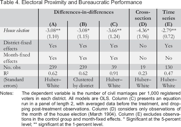
Notes: The dependent variable is the number of civil marriages per 1,000 registered voters in each district. All models are OLS. Column (C) presents an equation run in a panel of length 2, with averaged data before the treatment, and dropping post-treatment observations. Column (D) considers only observations of the month of the house election (March 1904). Column (E) excludes observations in the control group and month-fixed effects.

Significant at the 5-percent level;

significant at the 1-percent level.

DD estimates do not change when using the total number of civil marriages in each district as a dependent variable. The coefficient remains statistically significant when using OLS, Poisson, and negative binomial estimates (reported in the Appendix).

However, conventional standard errors may underestimate standard deviations of treatment effects, leading to an overestimation of significance levels (see Bertrand, Duflo, and Mullainathan 2004). Consequently, I apply two standard corrections. First, the model in column (B) presents robust standard errors clustered at the district level. Second, for the model in column (C), I collapsed time-series information into a pre-treatment and treatment period, dropping observations for months after the treatment. I then ran the equation on the averaged outcome in a panel length of 2. ¹⁷

This strategy works only when the treatment is applied at the same time in all treated districts (Bertrand, Duflo, and Mullainathan 2004), as is the case in the 1904 election.

The impact of elections on the number of civil marriages remains statistically significant in all three models, showing that statistical significance of the effect is not driven by an underestimation of standard errors.

Model (D) presents the estimated effect using a cross-section of districts in the month of March. This estimate is identical to the one presented in Table 3 and is included to facilitate comparison among alternative estimates. The model presented in column (E) compares the number of civil marriages in the month of the election with other months, only for districts in the treatment group. The coefficient for the treatment is −2.79 and statistically significant at the 1-percent level.

Estimates using three alternative strategies are not significantly different from each other. I interpret the similarity between these alternative estimators as informative of the robustness of my research design.

6 Robustness

In this section I present further tests to assess the validity of the results. A first simple potential objection is that fewer couples might want to marry near elections. Related to that, it could be argued that elections themselves decreased the performance of JOPs because of purely electoral duties such as registering voters, receiving voters at voting tables, and counting votes. To address these issues, I estimated the same models in Table 4 but used religious marriages per 1,000 registered voters as the dependent variable. Voter registration was carried out several months before elections and also in districts in the control group. Both JOPs and Catholic priests were in charge of receiving voters at voting tables and conducting vote counts (see Electoral Law no. 4161). ¹⁸

18
It is also unlikely that duties related to the legality of elections interfered with judges’ performance, because those claims were evaluated by the Special Powers Committee at Congress, and complaints were filed only in the district of San Cristobal (Diario de Sesiones de la Cámara de Diputados 1904).

Since religious and civil marriages are positively and significantly correlated in the sample (r = 0.42, p<0.00), they should constitute an acceptable false experiment. The fact that electoral districts and parochial divisions closely overlapped in the city of Buenos Aires makes this a valid comparison. Therefore, if elections led to a decrease in marriage rates because of reasons unrelated to bureaucratic political involvement, then we should see that they also have a negative impact on the number of marriages celebrated by the Catholic Church. Models presented in Table 5 show that this is not the case.

Table 5

False Experiment: Religious Marriages

	Differences-indifferences (A)	Cross-section (B)	Time series (C)
House election	-0.48 (0.61)	-1.01 (1.52)	-1.73^** (0.37)
District-fixed effects	Yes	No	Yes
Month-fixed effects	Yes	No	No
No. obs	114	12	72
R²	0.73	0.04	0.43

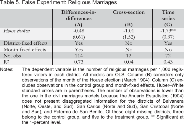
Notes: The dependent variable is the number of religious marriages per 1,000 registered voters in each district. All models are OLS. Column (B) considers only observations of the month of the House election (March 1904). Column (C) excludes observations in the control group and month-fixed effects. Huber–White standard errors are in parentheses. The number of observations is lower than the one in the civil marriages models because the Anuario Estadístico (1904) does not present disaggregated information for the districts of Balvanera (Norte, Oeste, and Sud), San Carlos (Norte and Sud), San Cristobal (Norte and Sud), and Palermo de San Benito. Of those eight missing districts, three belong to the control group, and five to the treatment group.

Significant at the 1-percent level.

Elections have no impact on the number of religious marriages celebrated in a given district. The coefficient is significant for the time-series model presented in column (C), ¹⁹ but not in the differences-indifferences or cross-section estimators presented in columns (A) and (B). These results support the notion that the impact of elections on civil marriages is indeed driven by the political involvement of JOPs. ²⁰

The coefficient is statistically significant because it does not consider the fact that religious marriages also dropped in the control group.

It should be noted that the false experiment presents conventional standard errors for the DD estimates. This is the most conservative approach, since this might bias statistical significance towards the rejection of the null hypothesis.

Of course, since there is no available or disaggregated information about religious marriages for some districts (three from the control group and five from the treatment group), the lack of statistical significance of the regression coefficients might be due to a reduction in sample size, which mechanically enlarges standard errors. To deal with this issue, I estimated the regressions of civil marriage presented in Table 4 while restricting the sample to those observations for which data on religious marriages exists. The negative impact of elections on civil marriages remains large (in fact, it becomes even larger than the estimate using the full sample) and statistically significant at the 1-percent level. ²¹

Results presented in the Appendix. The estimated coefficient for civil marriages ranges from −7.30 to −1.68 (at a 95 percent confidence level) and the one for religious marriages from −1.70 to 0.73 (at a 95 percent confidence level).

A second concern might be about the missing value for the district of Vélez Sarsfield (in the treatment group) in the month of the House election. To deal with this issue, I excluded this district from all samples of estimations of models presented in this paper. The direction and statistical significance of the coefficients of interest remained virtually unchanged (in fact, the absolute difference between experimental groups before and after elections became smaller).

A third potential objection would be about the seasonality of marriages. It could be argued that civil marriages consistently drop in the month of March in districts of the treatment group. Considering that elections were randomly distributed among districts, however, this is unlikely. Nevertheless, to deal with this issue, I calculated differences in means in the marriage rate between experimental groups in 1903 and their statistical significance, using simple t-tests. The difference (i.e. the effect of having an upcoming election) is not statistically significant in any month. ²²

Results not reported but available upon request.

A fourth way to assess the validity of the theory is to check whether the local effect of elections is higher in the least competitive districts. Results from previous elections could be used by bureaucrats to predict the competitiveness of each candidate's party. Given that the Senate election was carried out in all districts before the House election, bureaucrats would have been able to use that information to estimate the electoral competitiveness of each political party in the given upcoming election. If certainty is indeed important, as predicted by the Becker–Stigler model, then the political involvement of bureaucrats should be higher in the districts where the margin of victory in the preceding election was largest.

Table 6 presents separate differences-in-differences estimates for districts where the margin of victory – between the winner and the runner-up – in the Senate election (seven days before the House election) was above or below the median. Those below the median are always lower than 10, and those above vary between 11 and more than 67 percentage points. Results confirm the theoretical expectation and show that the political involvement of JOPs was appreciable only in the least competitive districts, and locally in the month of elections.

Table 6

Certainty and Bureaucratic Political Involvement

	Differences-in-differences
	(Margin > p50) (A)	(Margin < p50) (B)
House election	-4.65^** (1.24)	-1.76 (2.26)
District-fixed effects	Yes	Yes
Month-fixed effects	Yes	Yes
No. obs	120	119
R²	0.72	0.57

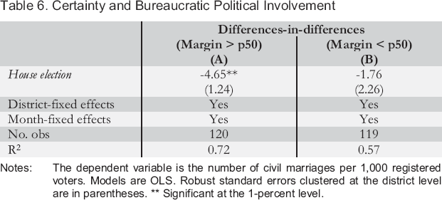
Notes: The dependent variable is the number of civil marriages per 1,000 registered voters. Models are OLS. Robust standard errors clustered at the district level are in parentheses.

Significant at the 1-percent level.

7 Conclusion

When do bureaucrats get involved in politics? Even though it is widely accepted that electoral fraud is frequently executed by public employees, most of the literature on electoral fraud assumes bureaucratic political involvement and focuses on discussing its execution. However, the execution of electoral fraud is only one of the tasks that politically involved bureaucrats undertake – and one that necessarily takes place on the day of the election. In this sense, the causes and temporal variation of bureaucratic political involvement demands more consideration. Are bureaucrats constantly involved in partisan matters or does this involvement vary over time?

In this article, I intended to fill this gap by building on a slight adaptation of the Becker–Stigler model of bureaucratic corruption (1974). I hold that incentives for the political involvement of bureaucrats increase when rewards are higher, and when information about future electoral performance is abundant. Electoral information is of vital importance because bureaucrats risk losing their jobs if they support a losing candidate.

Proximity to elections should increase both rewards and information, by two different mechanisms. First, as the salience of their political competitiveness increases near elections, candidates should be more willing to offer higher rewards to bureaucrats who support them. Second, political alliances and loyalties are clearest near elections, so the information available for bureaucrats to infer future electoral performance should be more accurate and more easily available. Therefore, bureaucrats can be expected to choose political involvement near elections.

I test this theory by exploiting a natural experiment. In Argentina in 1904, following the enactment of a new electoral law, elections for the House of Representatives were held in only half of the country's electoral districts, and these districts were chosen by a public lottery in Congress. Since the subsequent distribution of elections across districts can be presumed exogenous to bureaucratic political involvement, I collected monthly data from the city of Buenos Aires and estimated the effect of electoral proximity on the political involvement of justices of the peace (JOPs). To undertake this analysis, I assumed that the performance of public employees should decrease with political involvement – using the logic of “effect indicators” (Bollen and Lennox 1991).

All the results presented in this paper point in the same direction: the political involvement of JOPs increases locally in electoral months. I find a large, negative, and highly local effect of electoral proximity on the performance of JOPs, measured as the civil marriage rate. In the month of elections, districts experience as much as a 26-percent reduction in marriage rates when compared to the control group. I interpret this finding as evidence for the statement that bureaucrats are more likely to get politically involved near elections. The robustness of the empirical strategy is supported by the fact that similar conclusions are reached when using differences-in-differences, cross-section, and time-series estimators. Moreover, results appear not to be driven by spurious correlations associated with different dynamics for the treatment and control groups.

The theory of political involvement presented above predicts that the magnitude of rewards, electoral certainty, and bureaucratic wage levels determine the expected political involvement of bureaucrats. I presented evidence supporting the fact that electoral proximity, by boosting rewards and certainty, increases bureaucratic political involvement. This is an incomplete test of the presented theory. The isolation of the impact of bureaucratic wages on bureaucratic political involvement would require exogenous variation in wage levels. The Becker–Stigler model (1974) would lose explanatory power if higher-earning bureaucrats were not less likely to get involved in politics. Finally, research on the long-term impact of bureaucratic political involvement is certainly an important area for further study.

Footnotes

Appendix

Table A2.

Estimates Using the Restricted Sample

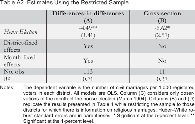
	Differences-in-differences (A)	Cross-section (B)
House Election	-4.49^** (1.41)	-6.62^* (2.51)
District-fixed effects	Yes	No
Month-fixed effects	Yes	No
No. obs	113	11
R²	0.71	0.37

Notes: The dependent variable is the number of civil marriages per 1,000 registered voters in each district. All models are OLS. Column (C) considers only observations of the month of the house election (March 1904). Columns (B) and (D) replicate the results presented in Table 4 while restricting the sample to those districts for which there is information on religious marriages. Huber–White robust standard errors are in parentheses.

Significant at the 5-percent level.

Significant at the 1-percent level.

References

Adcock

Robert

, and Collier

David

(2001), Measurement Validity: A Shared Standard for Qualitative and Quantitative Research, in: American Political Science Review, 95, 3, 529–546.

Ahuja

Sunil

(1994), Electoral Status and Representation in the Senate: Does Temporal Proximity to Elections Matter?, in: American Politics Quarterly, 22, 1, 104–118.

Alesina

Alberto

, and Tabellini

Guido

(2008), Bureaucrats or Politicians? Part II: Multiple Policy Tasks, in: Journal of Public Economics, 92, 426–447.

Alonso

Paula

(2010), Jardines Secretos. Legitimaciones Públicas, Buenos Aires: Edhasa.

Becker

Gary

, and Stigler

George J.

(1974), Law Enforcement, Malfeasance, and the Compensation of Enforcers, in: Journal of Legal Studies, III, 1–19.

Benton

Allyson L.

(2013), The Territorial Logic of Electoral Manipulation in an Electoral Authoritarian Regime: The Case of Mexico, unpublished manuscript, CIDE.

Bertrand

Marianne

, Duflo

Esther

, and Mullainathan

Sendhil

(2004), How Much Should We Trust Differences-in-Differences Estimates, in: The Quarterly Journal of Economics, 199, 1, 249–275.

Bollen

Kenneth

, and Lennox

Richard

(1991), Conventional Wisdom on Measurement: A Structural Equation Perspective, in: Psychological Bulletin, 110, 2, 305–314.

Botana

Natalio

(1985), El Orden Conservador, Buenos Aires: Editorial Sudamericana.

10.

Bowers

Jake

, and Panagopoulos

Costas

(2011), Fisher's Randomization Mode of Statistical Inference, Then and Now, 14 May, online: <www.jakebowers.org/PAPERS/BowPan-Fisher.pdf> (13 January 2016).

11.

Brownlee

James

(2007), Authoritarianism in an Age of Democratization, Cambridge, UK: Cambridge University Press.

12.

Bunce

Valerie J.

, and Wolchik

Sharon L.

(2011), Defeating Authoritarian Leaders in Postcommunist Countries, Cambridge, UK: Cambridge University Press.

13.

Canton

Darío

, and Jorrat

Jorge R.

(2004), Elecciones en la Ciudad 1864–2007. Tomo I (1864—1910), Buenos Aires: Instituto Histórico de la Ciudad de Buenos Aires.

14.

Cantu

Francisco

(2014), Identifying Irregularities in Mexican Local Elections, in: American Journal of Political Science, 58, 4, 936–951.

15.

Cárcano

Miguel A.

(1986), Sáenz Peña. La Revolución por los Comicios, Buenos Aires: Hyspamerica.

16.

Castro

Martín

(2004), Factional Struggle, Political Elites and Electoral Reform in Argentina, 1898–1912, PhD Dissertation, St. Anthony's College, Oxford University.

17.

Croley

Stephen P.

(1995), The Majoritarian Difficulty: Elective Judiciaries and the Rule of Law, in: University of Chicago Law Review, 62, 689–794.

18.

Diario de Sesiones de la Cámara de Diputados (1911), Honorable Cámara de Diputados Argentina.

19.

Diario de Sesiones de la Cámara de Diputados (1904), Honorable Cámara de Diputados Argentina, 2 May.

20.

Diario de Sesiones de la Cámara de Diputados (1882), Honorable Cámara de Diputados Argentina.

21.

Rafael

Di Tella

, and Schargrodsky

Ernesto

(2004), Do Police Reduce Crime? Estimates Using the Allocation of Police Forces after a Terrorist Attack, in: American Economic Review, 94, 1, 115–133.

22.

Rafael

Di Tella

, and Schargrodsky

Ernesto

(2003), The Role of Wages and Auditing During a Crackdown on Corruption in the City of Buenos Aires, in: Journal of Law and Economics, XLVI, 269–292.

23.

Dunning

Thad

(2012), Natural Experiments in the Social Sciences, Cambridge, UK: Cambridge University Press.

24.

Elling

Richard C.

(1982), Ideological Change in the United States Senate: Time and Electoral Responsiveness, in: Legislative Studies Quarterly, 7, 1, 75–92.

25.

Gehlbach

Scott

, and Keefer

Philip

(2008), Investment without Democracy: Ruling-Party Institutionalization and Credible Commitment in Autocracies, Working Paper, Social Science Research Network.

26.

Gehlbach

Scott

, and Simpser

Arturo

(2013), Electoral Manipulation as Bureaucratic Control, unpublished manuscript, Social Science Research Network, 18 November, online: <http://ssrn.com/abstract=2266988> (15 January 2016).

27.

Gerber

Alan S.

, Green

Donald P.

, and Kaplan

Edward H.

(2004), The Illusion of Learning from Observational Research, in: Shapiro

, Smith

, and Massoud

(eds), Problems and Methods in the Study of Politics, Cambridge, UK: Cambridge University Press, 251–273.

28.

Gerring

John

(2007), Is There a (Viable) Crucial-Case Method?, in: Comparative Political Studies, 40, 3, 231–253.

29.

Gomez

Silvana

(2013), Pa eso soy un ciudadano consciente: Caras y Caretas y la reforma electoral de 1902, in: Cambios y Permanencias, 4, 172–200.

30.

Gordon

Sanford C.

, and Huber

Gregory A.

(2007), The Effect of Electoral Competitiveness on Incumbent Behavior, in: Quarterly Journal of Political Science, 2, 107–138.

31.

Halperín Donghi

Tulio

(2007), La Formación de la Clase Terrateniente Bonaerense, Buenos Aires: Prometeo.

32.

Halperín Donghi

Tulio

(1992), Clase Terrateniente y Poder Político en Buenos Aires (1820–1930), in: Cuadernos de Historia Regional, 15, 11–46.

33.

Hora

Roy

(2001), The Landowners of the Argentine Pampas, Oxford: Oxford University Press.

34.

Huber

Gregory A.

, and Gordon

Sanford C.

(2004), Accountability and Coercion: Is Justice Blind When it Runs for Office?, in: American Journal of Political Science, 48, 2, 247–263.

35.

Jorrat

Jorge R.

, and Cantón

Darío

(1999), Buenos Aires en tiempo del voto venal: elecciones y partidos entre 1904–1910, Documento de Trabajo N° 8, Instituto de Investigaciones Gino Germani, Facultad de Ciencias Sociales, Universidad de Buenos Aires.

36.

Keele

Luke

, McConnaughy

Corrine

, and White

Ismail

(2006), Strengthening the Experimenter's Toolbox: Statistical Estimation of Internal Validity, in: American Journal of Political Science, 56, 2, 484–499.

37.

Larreguy

Horacio

, Montiel Olea

Cesar E.

, and Querubin

Pablo

(2014), The Role of Labor Unions as Political Machines: Evidence from the Case of the Mexican Teachers’ Union, unpublished manuscript, Harvard University and New York University.

38.

Lazarev

Valery

(2005), Economics of One-Party State: Promotion Incentives and Support for the Soviet Regime, in: Comparative Economic Studies, 47, 2, 346–363.

39.

Lehoucq

Fabrice

(2003), Electoral Fraud: Causes, Types, and Consequences, in: Annual Review of Political Science, 6, 1, 233–256.

40.

Levy

Jack S.

(2008), Case Studies: Types, Designs and Logics of Inference, in: Conflict Management and Peace Science, 25, 1–18.

41.

López

Mario Justo

(2005), De la República Oligárquica a la República Democrática, Buenos Aires: Lumiere.

42.

Losada

Leandro

(2012), El Mercado Matrimonial de las Familias Tradicionales Argentinas, 1900–1940. Algunas Dimensiones y Tendencias, in: Secuencia, 82, 129–151.

43.

Magaloni

Beatriz

(2008), Credible Power-sharing and the Longevity of Authoritarian Rule, in: Comparative Political Studies, 41, 4–5, 715–741.

44.

Magaloni

Beatriz

, and Kricheli

Ruth

(2010), Political Order and One-Party Rule, in: Annual Review of Political Science, 13, 123–143.

45.

Martinez-Bravo

Monica

(2014), The Role of Local Officials in New Democracies: Evidence from Indonesia, in: American Economic Review, 104, 4, 1244–1287.

46.

Morton

Rebecca

, and Williams

Kenneth

(2010), From Nature to the Lab: The Methodology of Experimental Political Science and the Study of Causality, Cambridge, UK: Cambridge University Press.

47.

Nichter

Simeon

(2008), Vote Buying or Turnout Buying? Machine Politics and the Secret Ballot, in: American Political Science Review, 102, 1, 19–31.

48.

Pereyra

Horacio J.

(1999), La Reforma de la Ley Electoral del Año 1902: Proyecto de Joaquín V. González, in: Sociohistórica, 6, 11–51.

49.

de Privitellio

Luciano

(2006), Representación Política, Orden, y Progreso: la Reforma Electoral de 1902, in: Política y Gestión, 9, online: <www.unsam.edu.ar/escuelas/politica/centro_historia_politica/pdf/texto1.pdf> (4 February 2016).

50.

Rundlett

Ashlea

, and Svolik

Milan W.

(2014), Deliver the Vote! Micromotives and Macrobehavior in Electoral Fraud, unpublished manuscript, University of Illinois at Urbana-Champaign.

51.

Sabato

Hilda

(2004), La Política en las Calles. Entre el Voto y la Movilización. Buenos Aires 1862–1880, Quilmes: Universidad de Quilmes.

52.

Simpser

Alberto

(2013), Why Governments and Parties Manipulate Elections: Theory, Practice, and Implication, New York: Cambridge University Press.

53.

Way

Lucan

(2006), Authoritarian Failure: How Does State Weakness Strengthen Electoral Competition?, in: Schedler

Andreas

(ed.), Electoral Authoritarianism: The Dynamics of Unfree Competition, Boulder and London: Lynne Rienner Publishers, 167–180.

54.

Wintrobe

Ronald

(1998), The Political Economy of Dictatorship, Cambridge, UK: Cambridge University Press.

55.

Wright

Gerald C.

, and Berckman

Michael B.

(1986), Candidates and Policy in the United States Senate Election, in: American Political Science Review, 80, 2, 567–588.

56.

Zarazaga , Rodrigo

S. J.

(2014), Brokers Beyond Clientelism: A New Perspective Through the Argentine Case, in: Latin American Politics and Society, 56, 3, 23–45.

57.

Zeballos

Estanislao S.

(1904), Vicios electorales y sociales, in: Revista de Derecho, Historia y Letras, XVIII, 142–150.

58.

Zeballos

Estanislao S.

(1902), Los Jueces, in: Revista de Derecho, Historia y Letras, XIV, 611–626.

59.

Zimmermann

Eduardo

(2009), Elections and the Origins of an Argentina Democratic Tradition, 1810–1880, Working Paper 365, Kellogg Institute.

60.

Zimmermann

Eduardo

(2007), Centralización, justicia federal y construcción del estado en la organización nacional, in: Revista de Instituciones, Ideas y Mercados, 46, 265–292.

61.

Zimmermann

Eduardo

(1996), La Formación de Abogados y Jueces en la Organización Nacional: Argentina, 1860–1880, paper presented at the Workshop “The History of Justice in Nineteenth-century Latin America”, Institute of Latin American Studies, University of London, 24 May.

Electoral Proximity and the Political Involvement of Bureaucrats: A Natural Experiment in Argentina,1904

Abstract

Keywords

Introduction

1 On the respective advantages of experimental research and observational research, see Gerber, Green, and Kaplan (2004) and Morton and Williams (2010). On natural experiments, see Dunning (2012).

2 In a recent paper, Zarazaga (2014) has shown that political operatives at the local level are valuable sources of information for their principals.

3 Unless otherwise noted, all translations into English are my own.

10 Boletín Oficial de la República Argentina, Año XII, No. 3078, 12 January 1904.

Table 2 Nomological Validation of Dependent Variable DV = Turnout (voters / registered voters) (1) (2) (3) Civil marriages -0.008 * (0.003) -0.005 * (0.001) Religious marriages 0.006 (0.003) District-fixed effects Yes Yes Yes Month-fixed effects Yes Yes Yes No. obs 39 24 23 R2 0.75 0.90 0.91

Footnotes

Appendix

References

1
On the respective advantages of experimental research and observational research, see Gerber, Green, and Kaplan (2004) and Morton and Williams (2010). On natural experiments, see Dunning (2012).

2
In a recent paper, Zarazaga (2014) has shown that political operatives at the local level are valuable sources of information for their principals.

3
Unless otherwise noted, all translations into English are my own.

10
Boletín Oficial de la República Argentina, Año XII, No. 3078, 12 January 1904.