Sage Journals: Discover world-class research

Abstract

Organizations in today’s supply chains strive for transportation activities optimization. However, transportation is a significant environmental impact activity. Particularly, road transportation is the highest emission rate source and the most widespread modality for last-mile delivery. In this context, the use of performance management tools, such as key performance indicators (KPIs), is a strategy to reach both economic-operative and environmental benefits. Among all KPIs, overall equipment effectiveness (OEE) is one of the most suitable KPIs to measure the utilization of an industrial asset. In the transportation sector, a variant of the OEE, known as the transportation overall vehicle effectiveness (TOVE), is used to define the performance of vehicle distribution activities, such as road transportation for last-mile delivery and urban logistics. Although TOVE is effective for evaluating vehicle performance in terms of administrative availability, operating availability, performance, and quality, the indicator does not take into the environmental impact related to road transportation activities. Literature has proposed several formulations to quantify transport carbon emissions, most of which are linear relationships to the distance travelled. However, these models are not suitable for assessing the TOVE performance of road transportation activities. This paper aims to compare the performance of last-mile delivery in terms of TOVE and carbon emissions evaluated with a distance travelled formulation in two different scenario systems. The comparison shows the inadequacy of TOVE in terms of environmental sustainability, as maximizing road transport performance while ignoring the environmental dimension excludes the minimization of CO₂ emissions. Therefore, the foundation for future developments of TOVE for sustainable road transportation can be established from this divergence.

Keywords

Transportation overall vehicle effectiveness carbon emissions environmental impact last-mile delivery performance measurement

Introduction

To efficiently meet customer needs while providing high service levels, organizations in today’s supply chains strive for transportation activities that are fast, accurate, flexible, and cost-effective.¹ However, transportation is also a major contributor to carbon emissions, and the transportation sector is the fourth largest source of environmental impact, with road transport accounting for 80% of emissions from freight and passengers.² Furthermore, to achieve net-zero emission targets, the transportation sector has the ambitious goal of reducing a large share of environmental emissions despite expectations of business growth.³ Against this backdrop, finding a balance between economic and environmental sustainability is crucial.⁴ Generally, three strategies can be implemented to improve the efficiency of an industrial process and reduce its environmental impact. The first strategy is direct mitigation, which involves reducing the emission rate produced by an asset or equipment, such as a vehicle. For example, this first strategy includes the revamping of an asset. The second is the replacement of the equipment with a new one characterized by better performance and lower consumption.^5–7 Finally, the third is the optimization of the entire process according to strategic and operational considerations. This paper focuses on the third strategy, as confirmed by Simons et al.,⁸ studies are missing holistic measures proposal of transportation efficiency toward sustainable development goals. In fact, most of these propose economic-operative performance measures while neglecting the impact that transportation activity has on the environment. To fill this gap, this paper evaluates the transportation process from both economic-operative and environmental perspective. Regarding economic-operative perspective, transportation overall vehicle effectiveness (TOVE) is a well-defined overall equipment effectiveness (OEE) variant to measure the performance of a distribution process⁹ and satisfy customer needs. However, TOVE does not take into account the environmental dimension, which is usually evaluated by using other consumption models. Consumption models involve the quantification of both pollutant emissions (e.g., particulate matter, nitrogen oxides, and sulphur oxides) and climate-altering substance emissions (e.g., CO₂). A widely used approach entails measuring the amount of CO₂ emissions based on the distance travelled by the vehicle.^10–12 Objectives targeting economic and environmental performance improvements may not be aligned as higher utilization of a vehicle leads to a greater environmental impact. Therefore, organizations lack a specific indicator for road transportation that considers both economic and environmental sustainability. From this perspective, this paper aims to highlight the need to develop a comprehensive indicator, laying the foundations for future research developments. The need of a comprehensive indicator is highlighted by the comparison of TOVE and CO₂ emissions in two different system scenarios. Specifically, it is intended to analyze two road distribution scenarios that implement different routing policies varying parameters of vehicle speed and maximum customer distance. The first scenario uses a first-in-first-out (FIFO) last-mile delivery policy whereby the first customer to request an order is the first to be served. In contrast, the second scenario proposes a last-mile delivery policy that follows a minimum shortest path (MSP) route to serve customers. The contribution of the paper is twofold. On one hand, it offers an updated list of OEE-based transportation efficiency indicators that may be useful for practitioners. On the other hand, the comparison of economic-operative and environmental measures lays the basis for researchers to develop a comprehensive indicator.

As a reminder, the structure of the article is as follows. In Literature review, a literature review is presented on key performance indicators (KPIs) specific to the OEE family for road transportation and models quantifying CO₂ emission on the road. Methodology outlines the methodology used. Results reports the results achieved. Finally, in Conclusion, the results are discussed, and conclusions and future developments are presented.

Literature review

This section provides the theoretical background of this study, investigating the existing literature on road transportation OEE-based indicators and carbon emission models. Specifically, Overall equipment effectiveness variants explore the proposed OEE variants for transportation activity, highlighting the pros and cons that led to the development of the KPI used in this study, namely, the TOVE. In addition, the section highlights the lack of OEE-based KPIs for the transportation sector that quantitatively account for the negative contribution of the logistics process to environmental impact. In Carbon emission models, the CO₂ emission quantification models are presented, including the assumptions and data availability under which they are typically used.

Overall equipment effectiveness variants

The OEE was originally created to implement Total Productive Maintenance as one of the lean techniques for efficient production.¹³ It calculates the productivity of assets in terms of availability, performance, and quality to track and improve an industrial system continuously. OEE is used in various industries, with variants such as Overall Tool Group Efficiency,¹⁴ Overall Throughput Effectiveness,¹⁵ and Overall Space Effectiveness.¹⁶ These are used to assess the performance of individual industrial assets, specific parameters in industrial processes like productivity, and layout performance, respectively.

In lean theory, transportation is regarded as one of the seven wastes and a non-value-adding activity that needs to be eliminated. However, service companies in the logistics sector view the delivery process as a key activity for customer satisfaction and, thus, economic growth. As a result, several variants of the OEE have been developed specifically for the transportation sector, all of which evaluate the performance and distribution of vehicles in terms of three major components: availability, performance, and quality. First, the Overall Vehicle Effectiveness (OVE) indicator was introduced to measure the performance of road freight vehicles based on the percentage of availability, the performance rate, and the quality mark.⁸ However, OVE is not suitable for scenarios with multiple destinations per delivery. OVE rewards less efficient routes from a fuel consumption point of view. In fact, the indicator gives better values to routes that minimize the total distance, regardless of the vehicle load that affects fuel consumption. A more appropriate performance estimate is to consider how much weight is moved and how much distance. To solve this problem, the Modified Overall Vehicle Effectiveness (MOVE) breaks down the performance component into route efficiency and time efficiency. The first component evaluates the efficiency of a route in terms of weight and distance compared to that consumed to cover the MSP route. Instead, the second component evaluates the efficiency of the route in terms of time, compared to the time for the MSP¹. Another alternative, Overall Transportation Effectiveness (OTE), measures economic-operative performance by identifying road transportation losses in higher detail. From the total time, OTE identifies the time spent by the company for some activities, such as planned standstill (e.g., maintenance, operator training, revision), routine losses (e.g., dock waiting time), and speed losses (e.g., traffic jams and kilometers empty).¹⁷ The above mentioned OEE-based indicators for transportation efficiency (OVE, MOVE, and OTE) evaluate performance excluding unscheduled time for shifts and company closures, and scheduled time for maintenance activities. However, such times are relevant to maintain assets in the operational phase.¹⁸ Therefore, another OEE-based indicator, namely TOVE, was developed by Villareal et al.¹⁹ to evaluate transportation performance on total calendar time, instead of only considering the net time of system closure and planned downtime. TOVE divides the organization’s activities into in-transit (IT) (i.e., activities involving active vehicle operation) and non-in-transit (NIT) (i.e., transport activities not involving the active use of vehicles) to assess logistics performance. As reported in Figure 1, TOVE evaluates availability by dividing it into administrative (AA) and operating availability (OA) and considers the performance (P) and quality (Q) of the systems in terms of IT activities.^9,19 Thus, TOVE is a well-established road transport-specific OEE variant.²¹ Table 1 summarizes the OEE variants found in the literature for transportation efficiency, along with reporting their identification (ID), reference, and pros and cons of their adoption.

Figure 1.

OEE and TOVE description.

Table 1.

OEE variants for the transportation sector.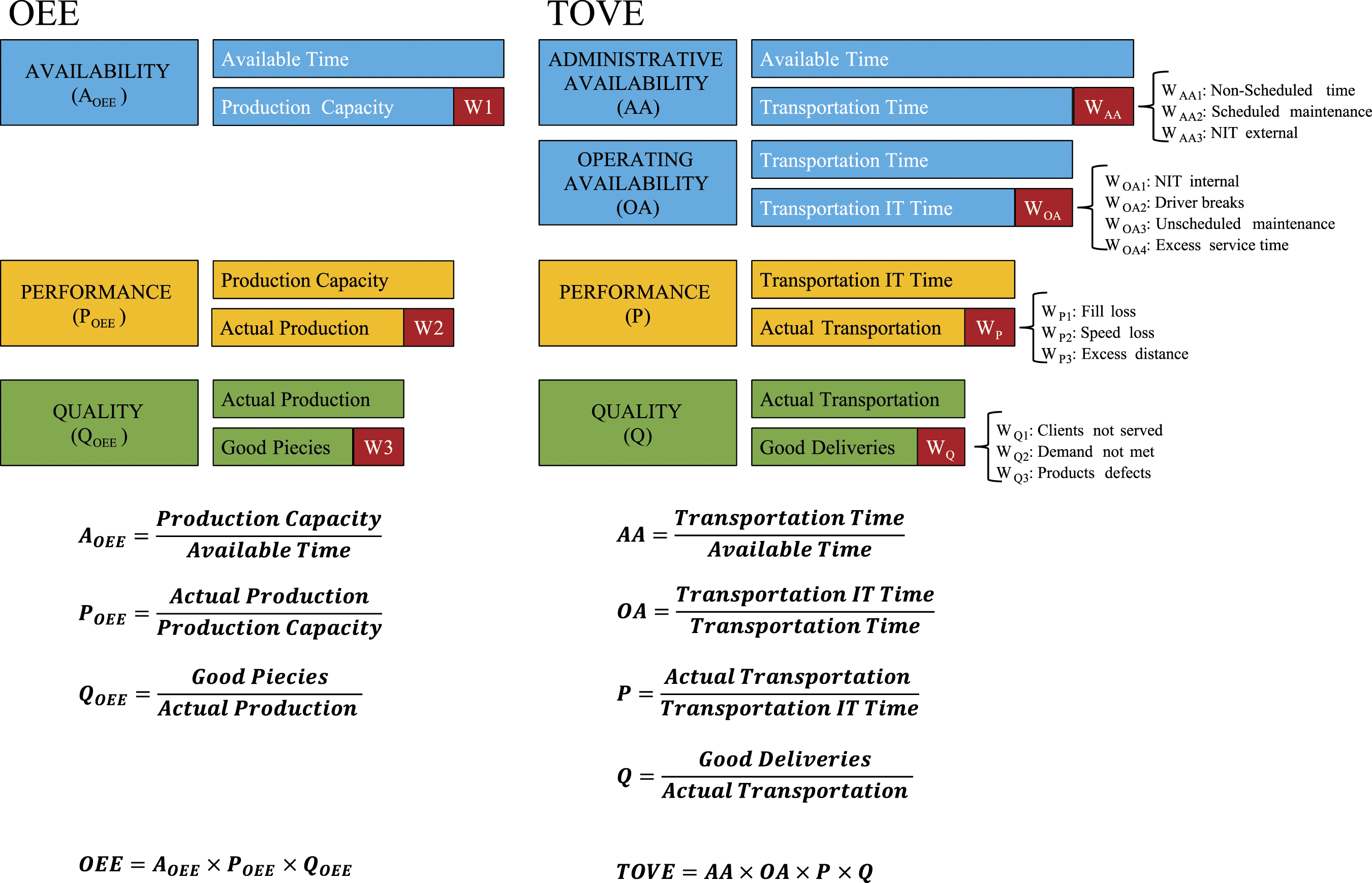

OEE variants	ID	Reference	Pros	Cons
Overall vehicle effectiveness	OVE	Simons et al.⁸	The first proposal of an aggregate indicator for measuring road transport efficiency. The indicator is based on the available time net of losses due to the five transportation losses (driver breaks, excess loading time, fill loss, speed loss, and quality)	Initially, the indicator was tested on a single case study, showing no statistical significance The indicator tends to reward less efficient routes in the case of multiple destinations
Modified overall vehicle effectiveness	MOVE	Sun et al.¹	It improves OVE by introducing a new component that quantifies in terms of vehicle utilization (weight to be carried) the ratio of proposed routes to optimal routes	The indicator was verified through a mathematical experiment. The validation of the measure is missing
Overall transportation effectiveness	OTE	Dalmolen et al.¹⁷	The indicator allows easier identification of losses from the total time of the interval considered The tool was validated through interviews with experts in the field	It quantifies routing effectiveness by calculating CO₂ emissions in little detail without providing implications of the relationships between operational performance and the environmental impact of transport
Transportation overall vehicle effectiveness	TOVE	Villareal et al.⁹	Compared to the other indicators, it considers total calendar time It classifies activities between IT and NIT which facilitates the identification of waste	It considers a transport system efficient if it is totally focused on transport activity. Therefore, it focuses only on economic-operative performance

As summarized in Table 1, the previously mentioned indicators do not take into account the domain of environmental sustainability. There are “sustainable” versions of OEE in the literature, but they are not designed for the transportation sector. Among the sustainable versions of OEE, an example is the Overall Greenness Performance (OGP), which evaluates the environmental performance of value-added activities based on four components: (i) company context for local environmental legislation and organizational culture, (ii) supply chain for supplier conditions and client requirements, (iii) consumption of non-value-added processes, and (iv) consumption of non-necessary non-value-added processes.^22–24 At a broader level, the Sustainable Overall Throughput Effectiveness (SOTE) KPI, incorporates environmental sustainability of production processes for series, parallel, converging, and diverging flows into the OEE components.²⁵ Finally, the Business Overall Performance and Sustainability Effectiveness (BOPSE), measures the relationship between Lean practices and Green production by combining OEE with a sustainability indicator that considers the three aspects of the Triple Bottom Line.²⁶ As stated by the literature review results, the performance management field lacks an OEE-based indicator to evaluate the environmental performance of transportation processes. On the other hand, several OEE-variants deal with economic-operative performance. Within this paper, TOVE was chosen as the indicator to measure the effectiveness of a road transportation process, even if it does not consider the environmental issue. The reason of the choice is that TOVE is a novel but well-established indicator that simultaneously improves on the criticalities and provides guidance on practical usefulness.

Carbon emission models

The amount of CO₂ emissions produced by a vehicle is directly proportional to the amount of fuel it consumes. In turn, fuel consumption is impacted by various factors, such as speed, road slope, traffic on the route, driver behavior, fleet size and mix, payload, empty miles, and green freight corridors.²⁷ Based on this, vehicle consumption models can be classified into three groups: macroscopic, microscopic, and factor emission models.²⁷ Macroscopic models estimate network-wide emissions using average network parameters. For example, MEET (Methodology for calculating transportation Emissions and Energy consumpTion) is a macroscopic model for calculating transport emissions and energy consumption per heavy-duty vehicle. The model evaluates the CO₂ emissions considering two different components, which are first determined through a series of regression functions and then merged into a single macroscopic function. The first component is the CO₂ rate calculated for standard conditions based on the distance travelled. The second component introduces some correction factors related to the gradient of the road and the load transported. Finally, the product of the two components gives the amount of CO₂ emitted.²⁸ Another macroscopic model is COPERT (COmputer Programme to calculate Emissions from Road Transportation), which estimates vehicle emissions by using specific regression functions for fuel consumption, where each of them depends on the vehicle weight. The function depends on speed and total distance.²⁹ However, macroscopic models do not estimate the instantaneous vehicle fuel consumption and emission rates at a more detailed level. To this end, microscopic models were developed. Microscopic models calculate emissions with more accuracy by considering instantaneous kinematic variables (speed and acceleration) or aggregated variables (e.g., time spent in traffic mode, cruise, and acceleration). Concerning microscopic models, Bowyer et al.³⁰ proposed several approaches, such as an instantaneous fuel consumption model (IFCM), a four-mode elemental fuel consumption model (FMEFCM), a running speed fuel consumption model (RSFCM), and an average speed fuel consumption model (ASFCM). However, both macroscopic and microscopic models require much information on traffic flows and the vehicle operating mode.²⁷ This information is not always available. Therefore, several authors have proposed factor emission models as valid and simpler approaches. Factor emission models appear to be unaffected by the variables of road transportation activities, such as environmental and traffic conditions, driver behavior, and vehicle operating conditions that are difficult to replicate.³¹ Generally, factor emission models use predefined emission factors to estimate CO₂ emissions, which are calculated per unit distance, per unit weight, per product, and per vehicle.³² Specifically, in the road transport sector, predefined emission factors measure the CO₂ consumption of transportation activities based on the distance travelled.³³ In contrast to TOVE, although factor models are widely used to quantify the environmental impact of road transport, they neglect economic-operative performance.

Overall, the performance management field lacks a specific indicator for road transportation that evaluates the optimization of economic and environmental dimensions. Moreover, to the best of the authors’ knowledge, the current scientific literature has not already provided a comparison between the performance of a road distribution system in terms of TOVE and factors models based on the travelled distance to evaluate CO₂ emissions. Hence, the aim of this article is to fill this gap by highlighting the inadequacy of TOVE and the importance of a comprehensive indicator that considers both economic and environmental perspectives.

Methodology

The methodology adopted in this work follows four sequential steps as shown in Figure 2. Firstly, the flow of activities is mapped, collecting quantitative and qualitative process information and splitting activities into IT and NIT ones. Secondly, the waste associated with each activity is identified. The wastes are associated with the four elements of TOVE that are, respectively, Administrative Availability (AA), Operating Availability (OA), Performance (P), and Quality (Q). Thirdly, the transportation route is planned, opting for an FIFO or an MSP policy. Finally, KPIs are calculated to assess both the economic-operative (TOVE) and environmental (CO₂ emission) performance of the last-mile delivery activities. Below, each step will be described in more detail.

Figure 2.

Methodological framework.

Mapping the flow is the initial methodological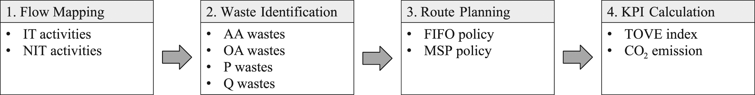 step. Lean principles are supported by flow mapping,³⁴ which makes it possible to map the stream of information, operators, and materials that have been or will be done as well as their proper sequence. Many flow mapping techniques may be taken into consideration, with the Value Stream Map (VSM) being a well-known and established tool.³⁵ In a VSM, activities are divided into value-added and non-value-added categories. Value-added activities are perceived by customers as necessary to satisfy their needs, unlike non-value-added activities. Among the latter, some non-value-added activities may be necessary and in support of value-added activities, while others are unnecessary. Non-value-added activities that are not necessary represent a significant waste for organizations that should therefore be eliminated. However, in the lean approach, transportation is regarded as a non-value-added activity. For this reason, the classification of activities on the basis of value was revised by Villareal et al.⁹ specifically for the transportation process. The classification groups activities in IT and NIT activities, to distinguish when transportation is conducted or not. This division of activities was used as a reference throughout this study. Then, traditional last-mile delivery process activities are considered. As a result, it is assumed that a distribution center receives a daily flow of supplies that are managed internally and dispatched as needed. The operators perform tasks, including unloading cargo, allocating shelves, selecting, and delivering items. The activities can be grouped following the classification of the logistics macro-phases which are inbound logistics, internal logistics, and outbound logistics.³⁶ Within this context, activities such as unloading goods, shelf allocation, picking, and delivery are carried out by the operators. Once the activities and their flow have been identified, it is therefore necessary to identify whether these activities are conducted in the most appropriate manner. It frequently happens that not all actions in a process are carried out to their full potential, and this implies waste creation. Within logistics field, many authors have identified wastes related to transportation process.^8,37,38 Specifically, according to the Villareal proposal,⁹ transportation wastes can be divided into four groups: i) AA, ii) OA, iii) P, and iv) Q wastes. AA wastes include time for which the transport activity is not conducted (W_AA1), time for periodic vehicle maintenance (W_AA2), and time due to other reasons for which the vehicle is stationary for non-operating reasons (e.g., route planning) (W_AA3). Availability losses for operational reasons that fall within the delivery phase are instead classified as OA wastes. OA wastes can be attributed to times when the vehicle is stationary despite the fact that it should be in motion (W_OA1), driver breaks (W_OA2), unplanned repairs (W_OA3), and excessive customer service time (W_OA4). However, operational waste does not consider the efficiency of the vehicle, which may lead to P wastes. In fact, three causes can lead to lower transportation performance. The first two concern losses in filling (W_P1) and speed (W_P2) such that the vehicle is forced to move with a reduced volume or quantity of elements and at a lower speed than expected. The third concerns time excesses due to longer distances (W_P3). In fact, it may happen that the delivery point is not the exact one for which the vehicle can be stopped, requiring a greater displacement of the operator. Finally, the last category of waste is the one related to the quality of service (Q), comprising wastes related to the percentage of customers not served (W_Q1), of demand not filled (W_Q2) due to inventory stock-outs, and of damaged products (W_Q3). The abovementioned wastes make it possible to quantify the four components of TOVE, which are shown in Table 2.

Table 2.

Components of TOVE related to different waste sources as represented in Figure 1.

Component	ID	Waste	Description
Administrative availability (AA)	W_AA1	Non-scheduled time	Time for which the transport activity is not performed
	W_AA2	Scheduled maintenance	Periodic scheduled maintenance
	W_AA3	NIT external	Time during which the vehicle is in non-in-transit state outside the transportation time
Operating availability (OA)	W_OA1	NIT internal	Time during which the vehicle is in non-in-transit state within the transportation time
	W_OA2	Driver breaks	All stops forced by some driver condition
	W_OA3	Unscheduled maintenance	Failures of vehicle elements that prevent normal or safe operation and require corrective action
	W_OA4	Excess service time	Additional time needed to provide the service requested by the customer
Performance (P)	W_P1	Fill loss	Filling losses of the vehicle according to an element, such as volume or quantity
	W_P2	Speed loss	Vehicle speed loss defined as the difference between the maximum permissible speed and the average speed
	W_P3	Excess distance	Additional distance required to provide the service requested by the customer
Quality (Q)	W_Q1	Clients not served	Customers for whom the order was not delivered due to administrative and operational inefficiencies
	W_Q2	Demand not met	Application not taken over due to lack of products
	W_Q3	Product defects	Non-conforming elements that are damaged in one or more activities performed by the distribution company

Route planning is the third step of the proposed methodology. To identify vehicle routes, let’s consider a group of customers scattered throughout a network, where a distribution center runs a product delivery vehicle. The first strategy considered is to follow the FIFO policy, which states that the first client who made the order will be the first to be served.³⁹ According to the FIFO policy, the sequence of served customers is not necessarily geographically organized in a logistic effective and efficient manner. The second strategy follows a MSP policy to identify the shortest path by minimizing the delivery route, without considering the order in which clients arrive. To solve this problem, there are methods for vehicle routing problems (VRPs) that define the best route by meeting a set of criteria.⁴⁰

\min \sum_{i, j \in V} c_{i j} x_{i j}

(1)

\sum_{i \in N} x_{i j} = 1 \forall j \in N

(2)

\sum_{j \in N} x_{i j} = 1 \forall i \in N

(3)

x_{i j} \in {0, 1} \forall i, j \in N

(4)

where i and j represent the starting and arrival points, respectively, while

x_{i j}

refers to the connecting path. In a network with N nodes, Equations (1)–(4) define a generic routing optimization problem. N stands for the total number of customers in the instance under consideration. The objective function (Equation (1)) considers the two constraints (Equations (2) and (3)) of each node (one incoming and one outgoing arc) and can take the value one if selected (if the connecting path is covered) or 0 if not. Based on the constraints, the objective function minimizes the total cost of the selected arcs that individually depart from i and reach j, whereas passing from

x_{i j}

has a cost value of

c_{i j}

. There are several heuristic approaches that identify feasible solutions since VRP falls within the category of NP-hard problems.⁴¹ In this article, the routing is determined by sequentially identifying the next unvisited node that is the closest to the preceding one.

The efficiency of the last-mile distribution actions in the two system scenarios is then measured using KPIs from an economic-operative and environmental point of view. TOVE and CO₂ emissions from road transportation are used as the KPIs for scenario evaluation. The assessment of TOVE has a similar formulation to the one of the OEE indicator (Figure 1). The best-case scenario for each component is that it can only assume the unit value. Because of the existence of waste, practical scenarios define lower levels. Each waste is identified in the TOVE component where it causes inefficiencies, as previously mentioned (see Table 2). On the other hand, the distance travelled is taken into account when calculating carbon emissions (Equations (5)). Practically, a light goods vehicle model with an emission factor ( $e_{f}$ ) of 0.230 Kg of CO₂ per km driven³⁵ was taken into consideration because of the absence of information on traffic flows and operational modes.²⁷ Moreover, this choice ensures the generality of the comparison between the two selected indicators. The total amount of CO₂ emissions is calculated as the sum of the product of the emission factor $e_{f}$ and the distance $d_{i j}$ travelled to reach consecutive points belonging to the customer set N. To reiterate, the primary goal of this work is to draw attention to the inadequacies of TOVE indicator in achieving the primary objective of green logistics, which is to minimize environmental impacts.⁴²

{E_{C O}}_{2} = \sum_{i, j \in N} e_{f} * d_{i j}

(5)

Results

The comparison between TOVE and CO₂ emission was conducted in two scenarios, one for FIFO strategy and one for MSP policy. Each scenario consists of two three-level variables, namely, the maximum acceptable distance of customers from the distribution center (30, 40, and 50 km) and the vehicle speed (40, 60, and 80 km/h).

The analysis generated a random distribution of 50 customers within a circle with a radius equal to the maximum acceptable distance from the distribution center, as shown in Figure 3. The last-mile delivery process is carried out by a single vehicle with a speed loss (W_P2) of 10%. The distribution center operates within a 12-h time interval, of which 8 h are dedicated to transportation activities. Prior to delivery, activities such as procurement, storage, truck loading, and periodic maintenance are performed. Once the allotted time for deliveries is completed, any undelivered products are unloaded and stored. The evaluation of the operational and environmental performance of the two scenarios is assessed using a discrete event simulation model. The activities on the nodes were linked logically in a sequence. Within the simulation model, the variables Delivery and C are used as state variables. Delivery is a Boolean variable that identifies the state of the last-mile delivery process, with a value of one indicating an active state and a value of 0 indicating an inactive state. This classification makes it possible to distinguish activities that are IT (Delivery equal to 1) from those that are NIT (Delivery equal to 0). The discrete status variable C indicates the total orders to deliver daily, that correspond to the number of customers to be served. The graphical representation of the simulation model is shown in Figure 4.

Figure 3.

Customer space distributed according to three levels of a concentric circle at the distribution center.

Figure 4.

Graphical representation of the simulation model.

The simulation model is controlled by a time variable T, which determines the state variable Delivery. At the beginning of the working day (T_open), NIT activities are performed, followed by the distribution activity starting at T_start and continuing until all customers are served (

C = 0

) or until the end of the delivery time (T_{finish delivery}). At the end of the day, final activities are carried out to conclude the working day at the T_close instant. Table 3 presents the event transition table, which illustrates the activities, their interrelationships, and the time distributions. The table also displays the state variables and the conditions that trigger their change, represented by dashed boxes in the graphic representation, while non-dashed boxes represent the change of state variables that do not require conditions.

Table 3.

Event transition table of the simulation model.

Event name	State change	Edge condition	Time delay (seconds)	ID	Next event
Start	C = 0 AND delivery = 0	Always	0		Unload incoming goods
Unload incoming goods	C = C_max	Always	Uniform (1200, 1800)	T_unloadIN	Place goods on a shelf
Place goods on a shelf	C --	C >0	Norm (120, 180)	T_all	Place goods on a shelf
		C = 0	0		Load vehicle
Load vehicle	C ++	C < C_max	Norm (30, 180)	T_load	Load vehicle
		C = C_max AND delivery = 1	0		Reach a costumer
Reach a costumer		C >0	F (distance; speed)	T_trans	Serve customer
Serve costumer	C --	Delivery = 1	Norm (120, 120)	T_serv	Reach customer
		Delivery = 0 OR C = 0	0		Return to DC
Return to DC		Always	F (distance; speed)	T_trans	Unload vehicle
Unload vehicle		C >0	Norm (30, 180)	T_unload	Place goods on a shelf
Place goods on a shelf	C --	Always	Norm (120, 180)	T_all	Unload vehicle
		C = 0	0		Finish

To build and run the simulation model, the following assumptions were considered:

• Scheduled maintenance activities are considered sufficient to avoid significant downtime in unscheduled maintenance activities (W_OA3),⁹

• a daily route design is implemented to maximize vehicle capacity, such that waste fill loss (W_P1) is negligible,⁴³

• a daily route design is implemented to minimize the routing distance, such that the excess waste distance (W_P3) and driver breaks (W_OA2) are negligible,⁴³

• demand is always met without backlog/backorder policies, such that waste demand not met (W_Q2) is negligible, and⁴⁴

• there are no handling errors in the loading and unloading vehicle activities, resulting in zero waste product defect (W_Q3).⁴⁵

After identifying the wastes and specifying the activities, the KPIs were measured. For each scenario, 10 simulation runs were executed for each combination of the two variables (distance and speed). In each simulation, 50 customers were randomly generated within a circle of radius equal to the maximum acceptable distance. The average values and deviations of the TOVE indicator and CO₂ emission were calculated, and the results are presented in Tables 4 and 5, respectively. Appendix A provides a more detailed view of the results for the two scenarios (FIFO and MSP policy) with varying parameters of maximum distance to the customer and vehicle speed.

Table 4.

Average values and standard deviation of TOVE results for both scenarios.

Scenario 1 (FIFO policy)				Scenario 2 (MSP policy)
Speed	Distance			Speed	Distance
Speed	30 Km	40 Km	50 Km	Speed	30 Km	40 Km	50 Km
40 Km/h, %;	13.55, 10.06	14.16, 11.16	9.37, 7.03	40 Km/h	22.59, 6.18	20.24, 7.96	18.01, 8.53
60 Km/h, %	15.60, 11.96	20.18, 12.50	16.73, 11.99	60 Km/h	22.97, 5.10	24.65, 5.42	22.02, 7.57
80 Km/h, %	17.60, 6.69	18.77, 10.72	18.35, 9.37	80 Km/h	23.98, 2.66	26.56, 4.96	25.70, 5.38

Table 5.

Average values and standard deviation of total KgCO₂ emissions for both scenarios.

Scenario 1 (FIFO policy)				Scenario 2 (MSP policy)
Speed	Distance			Speed	Distance
Speed	30 Km	40 Km	50 Km	Speed	30 Km	40 Km	50 Km
40 Km/h	136.03, 92.98	167.85, 103.38	177.87, 120.28	40 Km/h	55.68, 9.43	67.87, 15.30	78.12, 25.64
60 Km/h	143.06, 82.90	231.32, 105.31	250.95, 126.71	60 Km/h	64.56, 6.73	79.11, 11.99	94.73, 20.07
80 Km/h	179.14, 61.12	238.03, 118.03	265.87, 112.07	80 Km/h	71.21, 4.30	88.72, 7.89	102.42, 12.77

From a general perspective, the TOVE indicator tends to have lower values for longer delivery distances and slower vehicle speeds. In contrast, higher speeds typically result in relatively good TOVE values. Comparing the two scenarios, it becomes clear that optimizing the delivery route can yield significant benefits in terms of performance. Scenario 2, which minimizes the route and vehicle usage time, allows more customers to be served. On average, Scenario one served 27.13 customers, while Scenario two served 43.48 customers, representing 54% and 87%, respectively, of the maximum of 50 customers to be served. These results have a significant impact on the quality of the transport service, which is one of the four components of the TOVE indicator (Q).

Figure 5 provides a more detailed analysis of Scenarios one and two through a box plot representation of the TOVE components. Most of the TOVE components are independent of both vehicle speed and distance between customers and the distribution center. AA is similar for both scenarios as wastes are identified with the same assumptions and activities assume equal time distributions. OA assumes lower values for Scenario 2, with average values ranging between 66.86% and 81.01%, while Scenario one assumes average values ranging between 86.68% and 94.49% independently of vehicle speed and customer distance. The difference in average values between the two scenarios is due to a particular loss that exceeds service time. The greater the number of satisfied customers per time interval, the greater the probability of incurring a higher customer service time. This variation is driven by the strategic choice to optimize routes instead of distance and speed parameters. The only component of TOVE that depends on the maximum distance and speed parameters is the quality of the transport service (Q). As detailed results show, the average values of Q for Scenario one fall within an average range of 36%–64.60%, while in Scenario two the average range is between 69.60% and 99.60%. The difference in values is due to the strategic choice of route planning, which allows more customers to be satisfied in the same time interval with the same operating parameters. Furthermore, as expected, Q worsens as the maximum customer distance increases and improves as the vehicle speed increases, due to the transportation vehicle time that is dependent on these two parameters.

Figure 5.

TOVE components for Scenario 1 (a) and Scenario 2 (b).

Regarding carbon emissions, both scenarios exhibit the same pattern for each combination of variable levels. On average, Scenario one produces about 200 kg of carbon emissions, which is more than twice the value of Scenario 2. Average values are minimum when orders are processed within 30 km of the distribution center (i.e., the lowest level of the distance variable). The results demonstrate that the environmental impact is directly proportional to the vehicle speed. For the CO₂ emission model employed, which is solely a function of the distance travelled (Equation (5)), the increase in emissions is due to the greater number of customers served (and therefore Q value of the TOVE indicator). This justifies the maximum value assumed for both scenarios by both high levels of distance and vehicle speed. Finally, at the same levels, Scenario 2, which employs routing optimization to minimize the distance travelled (corresponding, in this case, to the only dependent variable of transport emissions), has lower values than Scenario 1.

It is possible to state that the two investigated KPIs assume high results for opposite pairs of values. TOVE reaches high values at the highest speed level. Instead, CO₂ emissions register low values at the lowest speed and distance levels. The trade-off is found for intermediate values. As shown in Tables 4 and 5, for Scenario 2, a good compromise is obtained for the combination of intermediate values of both analyzed variables. This evidence highlights the inadequacy of the TOVE performance indicator in optimizing both economic and environmental goals. The higher the value of the vehicle speed, the higher the number of customers served, and consequently the TOVE. This is reflected in the fact that the higher the number of customers served, the greater the CO₂ emissions of the transportation process.

Conclusion

Several studies have highlighted the importance of process efficiency in achieving economic goals while also addressing environmental concerns. In the transportation sector, these two factors are closely related, as increased transportation usage often leads to greater environmental impact. While the concept is well understood, studies on performance management lack comparisons between economic-operative and environmental indicators, which highlights the need for comprehensive indicators. This paper compares two indicators, TOVE and CO₂ consumption, and lays the groundwork for the future development of effective sustainable logistic indicators.

TOVE is a specific variant of the OEE family designed to quantify the economic and operational performance of road transportation at the calendar level. It consists of four components: administrative availability, operational availability, performance, and quality. On the other hand, CO₂ emissions measure the environmental impact of road transportation. The paper proposes a methodological framework to compare two scenarios that differ in their use of routing optimization policies. Each scenario is evaluated by combining (on three levels) the variables of the maximum distance of the customer and the average speed of the vehicle. A discrete-event simulation model replicating last-mile delivery on a random sample of 50 customers is used to assess the two scenarios for each combination of the variables.

Achieving a balance between economic and environmental goals is essential for ensuring sustainable and efficient transport operations. The result show that the two indicators outperform for opposite pairs of variables, with the trade-off being the respective intermediate levels. TOVE records high values for high speed levels, while CO₂ emissions (measured in kg) have low values for low levels of distance and low levels of vehicle speed. Therefore, there is a need to find a balance between the two KPIs to optimize both economic and environmental goals. This could involve finding optimal combinations of speed and distance levels that result in a good compromise between high TOVE values and low CO2 emissions. Among the four TOVE components, Q is the only one that depends on changing parameters and conditions OA. While TOVE is a well-established indicator for road transportation performance, it does not take environmental aspects into account. Therefore, the comparison presented in this paper lays the foundation for a new global KPI that takes into account both economic and environmental aspects.

From a practical perspective, this work identifies an updated list of indicators for assessing the performance of road transportation. However, the study also highlights limitations in the use of tools for measuring economic and environmental performance, as well as the assumptions made for evaluation. The factor emission model used to assess the impact of the activity on the environment is general and lacks detailed data. Future work could consider the use of microscopic or macroscopic models for assessments with a higher level of detail. Another alternative direction could be to incorporate additional environmental performance indicators into the analysis, such as energy consumption or air pollution, in order to provide a more comprehensive view of the environmental impact of the transportation process. Another limitation is the consideration of a single vehicle for last-mile delivery. Future development could involve the vehicle fleet, considering vehicles of different types and larger numbers. Finally, this work is limited to last-mile delivery with a single mode of transportation, leaving out other logistics activities. Future work could extend the comparison to a higher level by considering all logistic activities across a supply chain using different and combined transportation modes.

Supplemental Material

Supplemental Material - Assessing the adequacy of transportation overall vehicle effectiveness for sustainable road transportation

Supplemental Material for Assessing the adequacy of transportation overall vehicle effectiveness for sustainable road transportation by Saverio Ferraro, Alessandra Cantini, Leonardo Leoni, and Filippo De Carlo in International Journal of Engineering Business Management.

Footnotes

Authors contribution

All authors acknowledge their contribution according to the following criteria of International Committee of Medical Journal Editors authorship guidelines:

• Substantial contributions to the conception or design of the work; or the acquisition, analysis, or interpretation of data for the work;

• drafting the work or revising it critically for important intellectual content;

• final approval of the version to be published;

• agreement to be accountable for all aspects of the work in ensuring that questions related to the accuracy or integrity of any part of the work are appropriately investigated and resolved.

Declaration of conflicting interests

The author(s) declared no potential conflicts of interest with respect to the research, authorship, and/or publication of this article.

Funding

The author(s) received no financial support for the research, authorship, and/or publication of this article.

ORCID iDs

Saverio Ferraro

Alessandra Cantini

Leonardo Leoni

Filippo De Carlo

Supplemental Material

Supplemental material for this article is available online.

References

Sun

Mason

Disney

. MOVE: modified overall vehicle effectiveness. In: Proceedings of the 8th International Symposium of Logistics. Seville, Spain, 2003.

Intergovernmental Panel on Climate Change . Edenhofer

, (eds) In: Climate change 2014: mitigation of climate change: Working Group III contribution to the Fifth Assessment Report of the Intergovernmental Panel on Climate Change. New York, NY: Cambridge University Press, 2014, p. 1435.

Boullauazan

Sys

Vanelslander

. Developing and demonstrating a maturity model for smart ports. Marit Policy Manag 2022 May 25; 50(0): 447–465.

Brundtland

. “Report of the World Commission on environment and development:” our common future. New York: UN, 1987.

Cantini

Leoni

De Carlo

, et al. Technological energy efficiency improvements in cement industries. Sustainability 2021; 13(7): 3810.

Cantini

Leoni

Ferraro

, et al. Technological energy efficiency improvements in glass-production industries and their future perspectives in Italy. Processes 2022 Dec; 10(12): 2653.

Leoni

Cantini

De Carlo

, et al. Energy-saving technology opportunities and investments of the italian foundry industry. Energies 2021; 14(24): 8470.

Simons

Mason

Gardner

. Overall vehicle effectiveness. Int J Logist Res Appl 2004 Jun; 7(2): 119–135.

Villarreal

. The transportation value stream map (TVSM). Eur J Ind Eng 2012; 6(2): 216–233.

10.

Horvath

Environmental Assessment of Freight Transportation in the U.S. (11 pp). Int J Life Cycle Assessment 2006 Jul 1; 11(4): 229–239.

11.

Pinto

JTdM

Mistage

Bilotta

, et al. Road-rail intermodal freight transport as a strategy for climate change mitigation. Environ Dev 2018 Mar 1; 25: 100–110.

12.

Craig

Blanco

Sheffi

. Estimating the CO2 intensity of intermodal freight transportation. Transp Res D Transp Environ 2013 Jul 1; 22: 49–53.

13.

Nakajima

Introduction to TPM: total productive maintenance.(Translation). New York: Productivity Press, Inc, 1988. 129.

14.

Chien

Chen

, et al. Constructing the OGE for promoting tool group productivity in semiconductor manufacturing. Int J Prod Res 2007 Feb; 45(3): 509–524.

15.

Muthiah

Huang

. Overall throughput effectiveness (OTE) metric for factory-level performance monitoring and bottleneck detection. Int J Prod Res 2007 Oct 15; 45: 4753–4769.

16.

Chien

. Overall space effectiveness (OSE) for enhancing fab space productivity. IEEE Trans Semicond Manufact 2016: 1–1.

17.

Dalmolen

Moonen

Iankoulova

, et al. Transportation performances measures and metrics: overall transportation effectiveness (ote): a framework, prototype and case study. In: Proceedings of the 2013 46th Hawaii international conference on system sciences [internet]. Wailea, HI, USA: IEEE; 2013 [cited 2022 Apr 12]. p. 4186–95. Available from: http://ieeexplore.ieee.org/document/6480350/

18.

Jeong

Phillips

. Operational efficiency and effectiveness measurement. Int Jrnl of Op and Prod Mnagemnt 2001; 21: 1404–1416.

19.

Villarreal

Garza-Reyes

Kumar

. Lean road transportation – a systematic method for the improvement of road transport operations. Prod Plan Control 2016; 27(11): 865–877.

20.

Villarreal

Garza-Reyes

Kumar

. A lean thinking and simulation-based approach for the improvement of routing operations. Ind Manag Data Syst 2016; 116(5): 903–925.

21.

Garza-Reyes

Forero

JSB

Kumar

, et al. Improving road transport operations using lean thinking. Procedia Manufacturing 2017; 11: 1900–1907.

22.

Muñoz-Villamizar

Santos

Montoya-Torres

, et al. Environmental assessment using a lean based tool. In: Borangiu

Trentesaux

Thomas

, et al. (eds). Service Orientation in Holonic and Multi-Agent Manufacturing [Internet]. Cham: Springer International Publishing; 2018 [cited 2022 Apr 12]. p. 41–50. (Studies in Computational Intelligence; vol. 762). Available from: http://link.springer.com/10.1007/978-3-319-73751-5_4

23.

Muñoz-Villamizar

Santos

Garcia-Sabater

, et al. Green value stream mapping approach to improving productivity and environmental performance. Int J Product Perform 2019; 68(3): 608–625.

24.

Muñoz-Villamizar

Santos

Montoya-Torres

, et al. Measuring environmental performance of urban freight transport systems: A case study, 52. Sustainable Cities and Society, 2020.

25.

Durán

Capaldo

Duran Acevedo

. Sustainable Overall Throughputability Effectiveness (S.O.T.E.) as a Metric for Production Systems. Sustainability 2018 Jan 31; 10(2): 362.

26.

Abreu

Alves

Moreira

. The Lean-Green BOPSE Indicator to Assess Efficiency and Sustainability. In: Alves

Kahlen

Flumerfelt

, et al. (eds). Lean engineering for global development [internet]. Cham: Springer International Publishing, 2019. [cited 2022 Apr 12]. p. 259–91. Available from: http://link.springer.com/10.1007/978-3-030-13515-7_9

27.

Demir

Bektaş

Laporte

. A review of recent research on green road freight transportation. Eur J Oper Res 2014; 237(3): 775–793.

28.

Transport

Energy

Transport

, et al. Fourth framework programme: strategic research: meet: Methodology for calculating transport emissions and energy consumption. [Internet]. EU: European Union; 1999 [cited 2022 May 10]. Available from: https://policycommons.net/artifacts/292991/fourth-framework-programme/1176492/

29.

Kouridis

Gkatzoflias

Kioutsoukis

, et al. Uncertainty estimates and guidance for road transport emission calculations [Internet]. JRC Publications Repository. 2010 [cited 2022 May 10]. Available from: https://publications.jrc.ec.europa.eu/repository/handle/111111111/14202

30.

Bowyer

Akçelik

Biggs

. Guide to fuel consumption analyses for urban traffic management. Melbourne: Australian Road Research Board, 1984.

31.

López-Martínez

Jiménez

Páez-Ayuso

, et al. Modelling the fuel consumption and pollutant emissions of the urban bus fleet of the city of Madrid. Transp Res D Transp Environ2017 May 1; 52: 112–127.

32.

Soysal

Bloemhof-Ruwaard

Van Der Vorst

JGAJ

. Modelling food logistics networks with emission considerations: The case of an international beef supply chain. Int J Prod Econ 2014; 152: 57–70.

33.

Waltho

Elhedhli

Gzara

. Green supply chain network design: A review focused on policy adoption and emission quantification. Int J Prod Econ 2019 Feb 1; 208: 305–318.

34.

Cantini

De Carlo

Tucci

. Application of the lean layout planning system in a leather bags manufacturing plant and proposal of an approach to engage the company’s staff in the research of the layout solution In: Proceedings of the Summer School Web. Bergamo, Italy, 9 November 2020.

35.

Mason

Nieuwenhuis

Simons

. Lean and green supply chain mapping: adapting a lean management tool to the needs of industrial ecology. PIE 2008; 5(4): 302.

36.

Ferraro

De Carlo

Cantini

, et al. Green logistics for heavy equipment: a bibliometric analysis. In: Proceedings of the 27th Summer School “Francesco Turco”. Italy, 2022.

37.

Sutherland

Bennett

. The seven deadly wastes of logistics: applying toyota production system principles to create logistics value, 2007 Jan 1. Lehigh University Center for Value Chain Research, Lehigh.

38.

Sternberg

Stefansson

Westernberg

, et al. Applying a lean approach to identify waste in motor carrier operations. Int J Product Perform 2012; 62(1): 47–65.

39.

Cordeau

Dell’Amico

Iori

. Branch-and-cut for the pickup and delivery traveling salesman problem with FIFO loading. Comput Oper Res 2010 May 1; 37(5): 970–980.

40.

Ganesh

Nallathambi

Narendran

T t

. Variants, solution approaches and applications for Vehicle Routing Problems in supply chain: agile framework and comprehensive review. Int J Agil Syst Manag 2007 Jan; 2(1): 50–75.

41.

Sharma

Routroy

Yadav

. Vehicle routing problem: recent literature review of its variants. International Journal of Operational Research, 33(1), 1–31. https://doi.org/10.1504/IJOR.2018.094229

42.

Larina

Larin

Kiriliuk

, et al. Green logistics - Modern transportation process technology. Prod Eng Arch 2021; 27(3): 184–190.

43.

Villarreal

Garza-Reyes

Kumar

, et al. Improving road transport operations through lean thinking: a case study. Int J Logist Res Appl 2017; 20(2): 163–180.

44.

Villarreal

López

Rendón

, et al. A sequential truck transportation waste reduction scheme. In 2016. p. 1–10.

45.

Villarreal

Benavides-Peña

Garza-Amaya

, et al. Improving distribution efficiency to increase agility: an application to a Mexican company, 2017, In Proceedings of the International Conference on Industrial Engineering and Operations Management (pp. 873–884).

Supplementary Material

Please find the following supplemental material available below.

For Open Access articles published under a Creative Commons License, all supplemental material carries the same license as the article it is associated with.

For non-Open Access articles published, all supplemental material carries a non-exclusive license, and permission requests for re-use of supplemental material or any part of supplemental material shall be sent directly to the copyright owner as specified in the copyright notice associated with the article.

0.00 MB

0.33 MB