Sage Journals: Discover world-class research

Abstract

It is common in the integrated targeting inventory literature to assume 100% inspection. Yet, sampling inspection is still a valid alternative in numerous situations. Inspection time has been assumed negligible in the literature of integrated inventory and sampling inspection. Neglecting inspection time is unrealistic, especially when rejected lots are sent for 100% inspection. This research work integrates process targeting, production lot-sizing and inspection. Given a scenario of a producer and distributer, the objective is to determine the optimal mean setting at the producer, the production lot size to be produced and shipped to the distributor and the reorder point at the distributor under a given sampling inspection plan. To the best of the authors’ knowledge, sampling inspection and its associated costs are rarely addressed in integrated supply chain models, and have never been addressed in integrated models with controllable production rates. Numerical illustrations using an efficient solution technique are presented to highlight the impact of various model parameters. The results indicated that inspection time has a significant impact on the total cost of the developed model, especially, when tightened inspection plans are used.

Keywords

Two-echelon supply chain sampling inspection process targeting continuous review system

Introduction

Supply chain management is the centralized management of suppliers, materials, production facilities, distribution and customers. This is all linked together through the forward flow of material and backward flow of information.¹ Production, quality and maintenance are the main interrelated areas in any supply chain system. Due to their interdependence and to achieve global optimality, many researchers have studied the integration of more than one of these areas.^2,3 Joint economic lot-sizing is a primary aspect of coordination in supply chain, which was addressed for the first time by Goyal⁴ in the 1970. A research stream evolved over the following years to address different aspects of coordination and integration of decisions in supply chain. For a comprehensive review on integrated inventory models, the reader is referred to Glock.⁵

In this research work, we propose an integrated process targeting, joint economic lot-sizing and inspection model. The objective is to determine the process mean setting, reorder level and order quantity for a two-stage supply chain with sampling inspection. Products are manufactured through a variable production rate at the first stage then are sent in lots to a distributor’s warehouse at the second stage. A stochastic $Q - R$ model is used by the distributor to control the inventory level. Sampling inspection is used by the distributor for monitoring the quality of incoming lots. Note this assumes a predefined/given sampling scheme.

The earlier relevant research work (e.g., Darwish^6,7) assumed 100% inspection. Yet, sampling inspection is still a practical necessity since it has lower cost and represents the only applicable option whenever destructive testing is needed. Therefore, in contrary to the aforementioned research work, we consider inspection and relax the assumption of negligible inspection time. Also, we assume that inspection time is linearly proportional to the size of the produced lot. The effect of the inspection time will be significant whenever lots are rejected and sent to 100% inspection. This will result in the extension of the lead time due to100% inspection, and increased probability of running out of stock. We denote this time as the extended lead time.

The remainder of this paper is structured as follows: Section 2 provides a summary of the related literature. Section 3 illustrates the model assumptions and notations used throughout this paper. Section 4 provides a discussion on the effect of sampling inspection on the inventory model. Section 5 outlines the development of the proposed model. Section 6 present the proposed efficient solution technique. Section 7 presents a numerical example and a thorough sensitivity analysis. Finally, Section 8 provides conclusions, remarks and recommendations for future research.

Literature review

The integrated joint economic lot-sizing and quality control literature spans a plethora of topics. This section presents two streams of research that are closely relevant to the work at hand, namely; I) research works that address the integrated targeting inventory models II) research works that address integrated inventory and inspection sampling models.

Integrated process targeting and inventory control models

Process targeting models aim at determining the optimal process parameters to minimize the cost of items that do not meet the required specifications.^8,9 Gong et al.¹⁰ presented one of the earliest models that addressed the integration of process targeting and inventory control. They discussed the trade-offs in the process targeting problem and how it affects the process yield. Al-Fawzan and Hariga¹¹ studied the case of time-dependent process mean with lower specification limit on the produced items. Their developed model optimized process mean setting and both the lot sizes of the raw material and finished products. Later on, Hariga and AlFawzan¹² extended Al-Fawzan and Hariga’s¹¹ work to incorporate multiple markets, where the output of the production process can be sold to different customers in the same market, each with different quality requirements.

Darwish¹³ extended the single-vendor single-buyer inventory-targeting problem to consider joint determination of process mean and lot-sizing. The author showed the impact of the process mean on the vendor’s yield rate, which affects the production lot size and the number of unequal-sized shipments from the vendor to the manufacture. Later, Darwish and Abdulmalek⁶ extended this problem to consider a time-varying process mean. Alkhedher and Darwish¹⁴ addressed the integrated inventory-targeting problem with random demand. They assumed the produced items to have upper and lower specification limits and nonconforming items were scrapped. They concluded that demand variation should not be neglected in the integrated inventory-targeting problem. Darwish and Aldaihani¹⁵ studied the integrated inventory-targeting problem for a single-vendor multi-newsvendor supply chain. They demonstrated the importance of integration through a illustrative examples. The vendor sets the process mean, produces, and then ships to news-vendors who, at the end of the selling period, either run short of supplies or return surplus items to the vendor at a known rate.

Recent research works include: the possibility of order processing time reduction by including an investment cost to reduce order processing time from normal to a minimum duration,¹⁶ smart pricing and market segmentation,¹⁷ and addressing the case of stochastic demand.⁷

Integrated inventory and inspection sampling models

Lee and Rosenblatt¹⁸ provided one of the first joint inspection and inventory planning models, the fraction of nonconforming items per lot was assumed fixed and known. By relaxing this assumption, Zhang and Gerchack¹⁹ derived the optimal order quantity and fraction of lot to be inspected. Peters et al.²⁰ introduced an integrated inventory-inspection model, which determines the lot-sizing decision along with Bayesian quality control system, for a lot-by-lot attribute acceptance sampling plan.

Salameh and Jaber²¹ extended the classical EOQ model to a situation where the purchased items have imperfect quality, subject to 100% screening, items of secondary quality are sold in batches at the end of the screening process. Goyal and Cárdenas-Barrón²² provided a simplified way to solve Salameh and Jaber’s²¹ model. AlDurgam et al.²³ extended the classical production lot-sizing model to incorporate machining economics. Assuming 100% inspection, the authors demonstrated that machining parameters have an impact on the optimal lot size and the fraction of non-confirming units.

Cheung and Leung²⁴ developed a $Q - R$ model to manage the joint replenishment of a two-item inventory system. Ben-Daya et al.²⁵ developed an integrated stochastic inventory and inspection sampling model. They assumed that a buyer buys items with imperfect quality and uses inspection sampling to get rid of defective items.

For the joint economic lot-sizing systems, Wu et al.²⁶ considered the impact of inspection sampling, and order lead time reduction on a single-vendor single-buyer inventory system. Hsieh and Liu²⁷ considered a single-supplier single-manufacturer supply chain. The supplier performs outbound quality inspection and the manufacturer performs inbound and out bound quality inspection (before sending items to his customers). They studied the quality investment and inspection strategies of the system in four non-cooperative games. Sharifi et al.²⁸ studied the case of perishable products with imperfect quality and destructive testing. They determined the optimal lot size subject to an acceptance sampling plan.

Recently, Bouslah et al.²⁹ addressed a joint lot-sizing and inspection system, with an unreliable manufacturing process. Duffuaa and El-Ga’aly³⁰ presented a multi-objective process targeting model, the model aims at maximizing profit and product uniformity using the Taguchi loss function. They assumed a lower specification limit of the product and lot-by-lot acceptance sampling. Further, Duffuaa and El-Ga’aly³¹ showed that the inspection errors have a significant impact on the optimal problem solution. Recently, Duffuaa and El-Ga’aly³² extended Duffuaa and El-Ga’aly³¹ by considering multiple specification limits for two different quality grades of the same product. Chen et al.³³ presented a modified Kapur and Wang’s model with unequal target value. Taguchi’s quadratic quality loss function correlated to process capability indices (Cpm and Cpmk) is assumed. The author showed that the model with given Cpm value has less specification tolerance, larger process mean, and lower expected cost than those of the modified model with specified Cpmk. In a recent study, AlDurgam³ developed a stochastic dynamic programming model to study the interactions between production lot-sizing, quality inspection and maintenance for a single stage system, the author demonstrated the interactions between the maintenance, production and quality inspection parameters. Furthermore, the author characterized the optimal production and inspection policies.

Synthesis of both research streams

Most of the articles cited in Section 2.1 assumed 100% inspection. Also, most of the articles in Section 2.2 did not consider process targeting and neglected the effect of inspection time. In this article, we develop an integrated model that spans both research streams. Moreover, we introduce the concept of extended lead time as a consequence whenever the inspection time per unit is not neglected. The research works closest to the one at hand are those by Ben-Daya and Noman³⁴ and Darwish et al.⁷. Ben-Daya and Noman³⁴ didn’t consider process targeting and assumed negligible inspection time. Darwish et al.⁷ did not consider sampling inspection. The proposed model can be viewed as an integration of the models by Ben-Daya and Noman³⁴ and Darwish et al.⁷ and as an extension of the inspection model in Ben-Daya and Noman³⁴ by addressing non-negligible inspection time and different inspection schemes. Our work contributes to the literature through addressing a two-echelon supply chain involving a producer and distributer with sampling inspection. To the best of the authors’ knowledge, sampling inspection and its associated costs are rarely addressed in integrated supply chain models, and have never been addressed in integrated models with controllable production rates. Moreover, inspection time is always overlooked and neglected in the literature. In this article, the effects of sampling inspection including the inspection time will be considered, especially, when the incoming lots are rejected and subjected to 100% inspection.

Model assumptions and notations

In a two-echelon supply chain system, lots of fixed size (Q) are produced by a producer and dispatched to a distributer’s warehouse. The inventory system assumed here is a continuous review $(Q - R)$ model with random demand. Let X be the quality characteristic of interest for the product. It is assumed that X has the nature of the larger the better. That is, the product is considered to be accepted if $X \geq L$ ; otherwise, the product is rejected. There are numerous examples in the literature of products with a lower sided quality characteristic, such as glass sheets produced by glass manufacturers³⁵; the gold plating industry, where the thicker the layer of gold the better; and the steel galvanization industry.³⁶ The quality characteristic is assumed to follow a normal distribution with a pre-set parameter $μ_{x}$ and constant variance $σ_{x}^{2}$ . The probability of producing a nonconforming item will be

p = Pr (X \leq L) = Pr (Z \leq \frac{L - μ}{σ_{x}}) = \int_{- \infty}^{\frac{L - μ}{σ}} \emptyset (z) dz .

This section will develop the mathematical model for a two-echelon supply chain system involving a producer and a distributer. Figure 1 shows the inventory model of the distributer over time under sampling inspection. In this work, dispatched lots from the producer to the distributer are subjected to sampling inspection. A sample of size n is taken. If the number of defectives found is less than or equal to the threshold level, c, then the lot is accepted; otherwise, the lot is rejected. Rejected lots are sent to 100% inspection. The duration of the 100% inspection (Δ) is not negligible, and is assumed to be linearly proportional to the lot size Q (Figure1).

Figure 1.

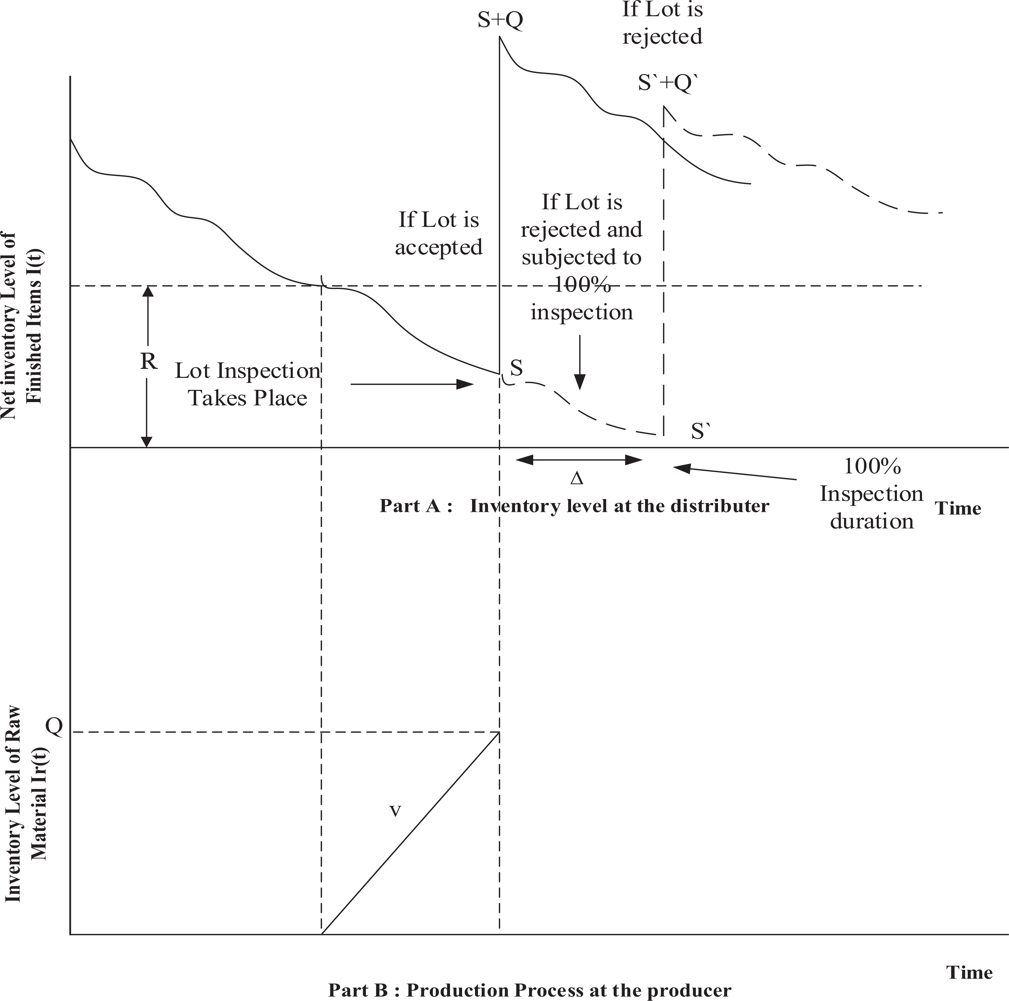
Inventory model over time for both the supplier and producer.

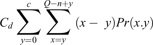
Sampling inspection trade-offs are extended to involve: the acceptance of defective items passing through the non-inspected portion of the accepted lots. The cost per unit of these items is c_d . And the time lost due to 100% inspection of the rejected lots. During this time, the inventory level is expected to drop to a lower level (S′ < S) due to the extension of the lead-time period with the additional 100% inspection duration (Figure 1). At the same time, the delivered lot size after 100% inspection (Q′) will be lower than the produced lot (Q) due to100% screening. The difference between Q and Q′ will not be replaced during the same cycle, since a reset up and reproduction is required. Therefore, this shortage will be treated in a similar way to the shortage encountered during lead time, and it will be backordered in subsequent cycles at a cost of rejection per unit c_r . Finally, the inspection cost per unit is considered. In this paper, the appropriate setting of the process parameters $Q$ , R, and $μ_{x}$ is simultaneously determined, such that the overall system cost is minimized.

To develop the model, the following assumptions are used:

Shortages are backordered;

The demand pattern is modeled by a normal probability distribution;

Inspection is free of errors;

Defective items after 100% inspection are not discarded, but they will be backordered in subsequent cycles;

The sampling inspection duration is negligible, but the 100% inspection duration is not. It is considered to be deterministic in nature and assumed to be proportional to the lot size Q;

The sampling inspection scheme is known and given.; and

In any cycle, the fraction of incoming defectives (p) is constant and depends on the setting of the production process parameter $μ_{x}$ .

The following notations will used throughout this paper:

A Setup cost of the producer per cycle.

c Number of defectives allowed per sample.

C Material cost per unit.

C_d Cost of accepting a defective item.

C_i Inspection cost per unit.

C_r Cost of rejecting a defective item during 100% inspection.

D Random variable that denotes demand rate.

h Inventory holding cost per unit of the finished item per unit of time.

l Lead-time duration.

L Lower specification limit.

n Sample size.

p Probability of producing a nonconforming item.

Q Lot size.

R Reorder point.

s Safety stock level before replenishment takes place.

$\bar{S} (s)$ Average expected shortage.

T Expected cycle length.

v Production rate of the producer.

x Random variable that denotes number of defectives per incoming lot.

y Random variable that denotes number of defectives per sample.

α Inspection time in hours per unit.

$Δ$ Deterministic variable that denotes 100% inspection duration.

$µ_{x}$ Process mean setting.

$π$ Shortage cost per unit short per unit of time.

$σ_{x}$ Standard deviation of the material used to produce an item.

$σ_{A}$ Standard deviation of the demand per unit time.

The effect of sampling inspection

In this section, we outline the effects of sampling inspection on the inventory cost model. Our main assumption throughout this model is that p is a decision variable controlled by the process mean setting $μ_{x}$ , and there is no drift in the process setting over time.

At the beginning, we need to define the following joint probability distribution $P r (x, y)$ of the two random variables x and y. Let $P r (x, y)$ be the joint probability distribution of x defectives per received lot Q, y defectives in a sample of size n. Using conditional probability, $P r (x, y)$ can be expressed as

P r (x, y) = P r (X = x) P r (y = y | X = x),

where $P r (X = x)$ is the marginal distribution of x defectives per lot. This marginal distribution is Binomially distributed with parameters p and Q. In addition, $P r (Y = y | X = x)$ is assumed to be Hypergeometric.³⁴

Lemma

The joint probability distribution Pr(x, y) can be stated as

$P r (x, y) = P r (y) . P r (x - y),$

y is a binomial random variable, $y = 0, ., n$ ,

x − y is a binomial random variable, $x - y = 0, \dots Q - n$ .

Proof

By replacing the right-hand side terms of $P r (x, y)$ with their binomial and hypergeometric forms respectively, we have

$Pr (x, y) = (\begin{matrix} Q \\ X \end{matrix}) p^{X} q^{Q - x} \frac{(\begin{matrix} X \\ y \end{matrix}) (\begin{matrix} Q - x \\ n - y \end{matrix})}{(\begin{matrix} Q \\ n \end{matrix})} .$

Simplifying the factorials, multiplying by $p^{- y} p^{y} q^{n - y} q^{- n + y}$ , and by further simplification:

$Pr (x, y) = (\begin{matrix} Q - n \\ X - y \end{matrix}) p^{X - y} q^{Q - n - x + y} (\begin{matrix} n \\ y \end{matrix}) p^{y} q^{n - y},$

$Pr (x, y) = Pr (y) . Pr (x - y) .$

In the following part, we follow a similar approach to that of Ben Daya et al.²⁵ to evaluate our inspection-related costs of our model.

Case 1: If the lot is accepted

The cost of inspection is the cost of taking a sample of size n and inspecting it; this is given by

$C_{i} n \sum_{y = 0}^{c} \sum_{x = y}^{Q - n + y} P r (x . y) = C_{i} n P r (y \leq c) .$
1

The cost of defective items passing through the non-inspected portion of the accepted lot is given by

$C_{d} \sum_{y = 0}^{c} \sum_{x = y}^{Q - n + y} (x - y) P r (x . y)$

Replacing $Pr (x, y) with Pr (y) . Pr (x - y)$ , and letting x − y = R gives

$C_{d} \sum_{y = 0}^{c} \sum_{R = 0}^{Q - n} (R) Pr (y) P r (R) = C_{d} (Q - n) p P r (y \leq c) .$
2

Case 2: If the lot is rejected

The cost of inspection will cover not only the sample of size n but also the remaining portion of the lot, $Q - n$ , that has to go for 100% inspection. This is expressed as

$C_{i} Q \sum_{y = c + 1}^{n} \sum_{x = y}^{Q - n + y} P r (x . y) = C_{i} Q - C_{i} Q P r (y \leq c) .$
3

The rejected items resulting from 100% inspection will not be replaced during the same cycle, but instead, they will be backordered at a cost per unit C_r . This cost could either be set to be equal to the penalty cost per unit short $π$ or have a different value. The expected cost of rejected units after 100% inspection is given by

$C_{r} \sum_{y = c + 1}^{n} \sum_{x = y}^{Q - n + y} (x - y) P r (x . y) .$

Simplifying in a similar manner to (2) gives

$C_{r} (Q - n) p P r (y > c)$

or

$C_{r} ((Q - n) p - (Q - n) p P r (y \leq c))$
4

Combining the costs in (1) through (4) gives the following expression for the expected quality cost:

$\begin{matrix} Quality costs : C_{i} Q + C_{r} (Q - n) p \\ + (Q - n) P r (y \leq c) ((C_{d} - C_{r}) p - C_{i}) . \end{matrix}$
5

The effect of sampling inspection on the received lot size Q

The reduction in the lot size Q will be realized from the defectives discarded from the inspected sample if the lot is either accepted or rejected and from the defective items resulting from the 100% inspection of the uninspected portion of the rejected lot, that is,

$\sum_{y = 0}^{n} \sum_{x = y}^{Q - n + y} y P r (x, y) + \sum_{y = c + 1}^{n} \sum_{x = y}^{Q - n + y} (x - y) P r (x, y)$

By further simplification,

$n p + (Q - n) p P r (y > c)$

or equivalently,

$Q p - (Q - n) p P r (y \leq c)$

Therefore, the expected quantity delivered due to sampling is

$\bar{Q} = Q - [Q p - (Q - n) p P r (y \leq c)]$
6

The effect on the safety stock level(s)

The safety stock level, s, changes according to the acceptance or rejection of the lot. If the lot is accepted, then $s = R - D l$ , while if the lot is rejected, the safety stock will drop further, and it will be given as $R - D (l + Δ) .$ That is,

$s = \{\begin{matrix} R - D l, Pr (y \leq c) \\ R - D (l + Δ), Pr (y > c) \end{matrix}$

Hence, the expected safety stock level is

$\bar{s} = R - D l - D ΔPr (y > c)$

or equivalently,

$\bar{s} = R - D (l + Δ) + D ΔPr (y \leq c) .$
7

The effect of sampling inspection on the inventory cycle time

The reduction in the lot size when the lot is accepted is due only to the defective items discarded from the sample. Thus, the delivered quantity is $Q - n p$ . In contrast, the reduction in the delivered lot size due to rejection because of the defectives discarded from the inspected sample and defectives discarded from the remaining portion of the lot is $Q p$ . Hence, the quantity delivered is $Q - Q p$ . The cycle length, T, is given as

$T = \{\begin{matrix} \frac{Q - n p}{D}, P r (y \leq c) \\ \frac{Q - Q p}{D} + Δ, P r (y > c) \end{matrix} .$

Hence,

$E (T) = \frac{\bar{Q}}{D} + Δ P r (y > c)$

or equivalently,

$E (T) = \frac{\bar{Q} + ΔDPr (y > c)}{D}$
8

Model development

In this section, we formulate the cost model by examining the costs associated with it for all the involved terms. The renewal theorem is used through adding inventory-related costs and dividing them by the expected cycle time in (8). The associated costs are given as follows.
1. Setup and material costs per unit of time at the manufacturer: A setup cost, A, is incurred once per cycle. The expected cost of material used per lot is $C Q μ_{x}$ . Thus, the expected setup and material costs per unit of time are equal to $(A + C Q μ_{x}) / E (T)$ . Substituting for $E (T)$ using (8) gives:

$\frac{D (A + C Q μ_{x} .)}{\bar{Q} + ΔDPr (y > c)}$
9

2. Holding cost per unit of time at the manufacturer and distributor: The average on-hand inventory for the $Q - R$ system at the distributor is $Q / 2 + s$ . However, with sampling inspection, depending on whether the lot is accepted or rejected, there are two possible values for both Q and s. In developing equations (7) and (8), we have considered the respective value of Q and $s$ that will take place in both cases. Therefore, the average on-hand inventory can be shown to be $E (Q) / 2 + E (s)$ or $\frac{\bar{Q}}{2} + \bar{s}$ . For the production side, the inventory starts to build up at a rate of v once an order is received and stops once Q units are produced. Thus, the average on-hand inventory per unit of time is $\frac{Q^{2}}{2 v E (T)}$ and the total holding cost per unit of time is

$h (\frac{\bar{Q}}{2} + \bar{s} + \frac{Q^{2}}{2 v E (T)})$

Substituting (6), (7) and (8) gives

$\begin{matrix} h (\frac{Q - [Q p - (Q - n) p P r (y \leq c)]}{2}) \\ + R - D (l + Δ) + D Δ P r (y \leq c) \\ + \frac{D Q^{2}}{2 v (Q - [Q p - (Q - n) p P r (y \leq c)]) + Δ D P r (y > c))} \end{matrix}$
10

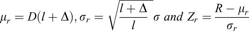
3. Shortage cost per unit of time at the distributor: The inventory system is subjected to shortages whenever the demand during lead time exceeds the reorder point, R. The expected number of shortages per cycle for the $Q - R$ system is given as

$S (z) = σ L (Z)$

where

$Z = \frac{R - μ}{σ}$

and $μ = D l$ is the mean of the lead time demand, $σ$ is the standard deviation of the lead time demand, and $L (z)$ is the standardized normal loss function.

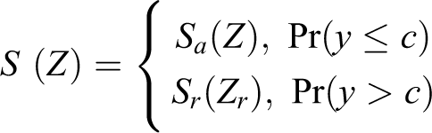
In our model, we must distinguish between shortages encountered when a lot is accepted versus those when a lot rejected. The distinction has to be made because of the additional 100% inspection period, $Δ$ , in the case of lot rejection. The parameters when the lot is rejected are as follows:

$μ_{r} = D (l + Δ), σ_{r} = \sqrt{\frac{l + Δ}{l}} σ a n d Z_{r} = \frac{R - μ_{r}}{σ_{r}}$

The suffixes r and a are added to denote rejection and acceptance, respectively; thus, shortages due to rejection are denoted by $S_{r} (Z_{r})$ , whereas shortages under acceptance are denoted by $S_{a} (Z)$ . The difference between $S_{a} (Z)$ and $S_{r} (Z_{r})$ is the use of different parameters. Hence, the shortage is expressed as

$S (Z) = \{\begin{matrix} S_{a} (Z), Pr (y \leq c) \\ S_{r} (Z_{r}), Pr (y > c) \end{matrix}$

Therefore, the expected shortage per unit of time is:

$\frac{π \bar{S} (Z)}{E (T)} = \frac{π D (S_{a} (z) Pr (y \leq c) + S_{r} (Z_{r}) Pr (y > c))}{\bar{Q} + ΔDPr (y > c)}$
11

The expected total cost per unit of time is the sum of the quality costs, setup costs, holding costs and shortage costs given by the equations (5), (9), (10) and (11), respectively, and by using (6), gives:

$\begin{array}{l} T C (Q, R, μ) = \frac{D (A + C Q μ_{x}) + π D (S_{a} (z) Pr (y \leq c) + S_{r} (z) Pr (y > c))}{Q - [Q p - (Q - n) p P r (y \leq c)] + ΔDPr (y > c)} \\ + \frac{C_{i} D Q + C_{r} D (Q - n) p + D (Q - n) P r (y \leq c) ((C_{d} - C_{r}) p - C_{i})}{Q - [Q p - (Q - n) p P r (y \leq c)] + ΔDPr (y > c)} \\ + h (\frac{Q - [Q p - (Q - n) p P r (y \leq c)]}{2} + R - D (l + Δ) + D Δ P r (y \leq c) + \frac{D Q^{2}}{2 v (Q - [Q p - (Q - n) p P r (y \leq c)]) + Δ D P r (y > c))}) \end{array}$

To simplify this expected total cost rate equation, we assume that the sample size, n, is negligible relative to the lot size $(Q > > n)$ . In addition, we assume that the inspection duration is linearly related to the lot size, that is, $Δ = α Q$ . Finally, as Figure 1 shows, $l = Q / v$ . This gives

$\begin{array}{l} T C (Q, R, μ) \\ = \frac{D (A + C Q μ_{x}) + π D (S_{a} (z) Pr (y \leq c) + S_{r} (z) Pr (y > c))}{Q (1 - (p - α D) (Pr (y > c))} \\ + \frac{C_{i} D Q + C_{r} D Q p + D Q P r (y \leq c) ((C_{d} - C_{r}) p - C_{i})}{Q (1 - (p - α D) (Pr (y > c))} \\ + h \frac{Q (1 - p P r (y > c))}{2} + R - \frac{D Q}{v} - α D Q P r (y > c) \\ + \frac{D Q^{2}}{2 v Q (1 - (p - α D) (Pr (y > c))} \end{array}$
12

Model analysis and solution procedure

This section presents an efficient solution technique for the model in Section 5. The decision variables are the order quantity (Q), the reorder level (R) and the process mean of the manufacturer ( $µ_{x}$ ). To determine the optimal values of these decision variables, we need to find an expression for each term at which the total cost vanishes. This is achieved by taking the derivative for each term and setting it to zero. By observing equation (12), it can be seen that $µ_{x}$ appears in various forms, either implicitly, as for the parameters p, $P r (y \leq c)$ , or even in an explicit manner. Therefore, it is not possible to have a first derivative for it. Working out the other two, we have

$\frac{\partial T C}{\partial Q} = 0 .$

$\begin{array}{l} - \frac{A D + π D (S_{a} (R) Pr (y \leq c) + S_{r} (R) Pr (y > c))}{B Q^{2}} \\ + h (\frac{v B (1 - p P r (y > c) - 2 B D (1 + α v P r (y > c)) + D}{2 v B}) \\ + \frac{π D^{2}}{B Q v} (Pr (y \leq c) (1 - Φ (Z)) + Pr (y > c) (1 + \propto v) (1 - Φ (Z_{r})) \\ = 0 \end{array}$
13

$\frac{\partial T C}{\partial R} = 0,$

$Pr (y \leq c) Φ (Z) + Pr (y > c) Φ (Z_{r}) = \frac{π D - h Q^{} B}{π D},$

where:

$B = 1 - (p - α D) Pr (y > c)$

$Z = \frac{R - D (Q / v)}{σ}$ , $Z_{r} = \frac{1}{\sqrt{1 + \propto v}} (Z - \frac{\propto Q D}{σ})$ ; applying the above for Z and Z_r* , we have:

$\begin{matrix} Pr (y \leq c) Φ (Z) + Pr (y > c) Φ (\frac{1}{\sqrt{1 + \propto v}} (Z - \frac{\propto Q D}{σ})) \\ = \frac{π D - h Q^{} B}{π D} \end{matrix}$
14

The presence of Q in the Z terms (Z and Z_r* ) gave the last term in equation (13). The derivative of $S (.)$ can be found by using its respective normal loss function, that is, $S (z) = σ L (z)$ and then by using the chain rule. When taking the derivative with respect to R, there will be two cases for Z. It can be easily verified that the maximum value equation (14) can take is 1.0. Thus, to have a feasible solution for equation (14), the right-hand side, $\frac{π D - h Q^{} B}{π D}$ , has to be less than or equal to 1. Hence,

$h Q B \leq π D, o r$

$Q \leq \frac{π D}{h B}$
15

Note that $B \geq 0$ . Equation (15) will set an upper limit for Q at any given pre-set value $µ_{x}$ . The inspection time per unit α has a clear effect on the feasible region of equation (14). If α is too small ( $α \to 0$ ), then equation (14) reduces to $Φ (Z) = (π D - h Q^{} B) / π D$ and a unique solution is found. In contrast, if α is extremely large ( $α \to \infty$ ), then $Z_{r} \to - \infty$ ; therefore, equation (14) becomes $Pr (y \leq c) Φ (Z) = (π D - h Q^{} B) / π D$ .This leads to the distortion of the feasible space. Therefore, a unique feasible solution is no longer guaranteed.

Equations (13) and (14) are not explicit in the variables Q and R. Therefore, to find a root for both equations, a search method is used. For equation (14), we use a simple search method over the range of Z ∈ [−3,3.9] at an increment of $δ$ . The search starts at Z = −3 and continues until the value obtained for the equation is close enough to the right-hand side within an acceptable margin of error. If such value does not exist, then set Z = 3.9 and $R = \frac{D Q}{v} + 3.9 σ$ . To determine the root for equation (13), the bisection method is used. This is a simple derivative-free method that requires bracketing the variable within two points with opposite function signs. To find the bracket limits, a simple search at a predetermined step size is used. This search will be conducted over the range (0, $minimum [\frac{π D}{h B}, D]$ ]) till a point K exists such that $\frac{\partial T C (K)}{\partial Q} > 0$ . If K does not exist, then $Q^{} = minimum [\frac{π D}{h B}, D]$ . The procedure for determining the optimal solution calls for letting $µ_{x}$ be controlled by a line search method. Here, we use the interval-halving method. This method is simple, derivative free and exhibits rapid convergence (Bazaraa et al. 1993). We start by bracketing $µ_{x}$ such that $µ_{x} \in [L, L + 3 σ_{x}]$ . We believe the bracket limits are adequate as they ensure the proportion of defectives will vary between almost 0 and 50%. During any iteration of the interval-halving algorithm, the corresponding $Q^{}$ and $R^{}$ values are determined using an iterative procedure that cycles between equations (13) and (14) until the values of Q and R are close enough within two subsequent iterations. The starting point of $Q = Q_{0}$ is assumed to be the economic production quantity, or $Q_{o} = \sqrt{\frac{2 A D}{h (1 - \frac{D}{v})}}$ . The iterative algorithm is as follows:

At any given $µ_{x}$ determine $Q^{}, a n d R^{}$ by the following procedure.
Step 1: Set Q_o to be equal to the $E P Q = Q_{o} = \sqrt{\frac{2 A D}{h (1 - \frac{D}{v})}}$ .

Step 2: Using the search method via equation (14), determine the value of R_i that corresponds to Q_i , where i represents the iteration number.

Step 3: Using the bisection method via equation (13), determine a new value for Q_i that corresponds to R_i from step 2.

Step 4: Using the value of Q_i from step 3, compute a new value for $R_{i}$ using the search method via equation (14).

Step 5: Repeat steps 3 and 4 until two successive values of $R_{i}$ and Q_i are approximately equal.

Step 6: The last values for $R_{i}$ and Q_i coming from step 5 are the optimal values of $Q^{}, and R^{}$ at any given $µ_{x}$ .

Numerical results

Below is a numerical example solved using the method outlined in Section 6. The goal here is to study the effect of the main model parameters and highlight various managerial insights. Unless otherwise specified, the following data are assumed throughout this section: L = 1.00, $σ_{x} = 1:00$ , $v = 500$ , $A = 100, D = 50 000, C_{i} = 1.25, h = 5, C_{d} = 30, C_{r} = 40, π = 20, α = 0.25 h r / u n i t, n = 89, c = 2, σ_{A} = 2000 a n d C = 1$ . We assume that the system operates 10 hours per day and 260 days per year. The inspection time per unit has to be converted to a yearly basis, considering the number of hours available per year. During our search for the proper Z value in equation (14) we used a fine value of δ = 0.0001. The numerical illustrations are carried out in the following sequence: First, we study the effect of inspection time over the model decision variables, assuming various sampling plans. Then, we study the effect of selected cost parameters using a fixed sampling plan.

Quality sampling plan and inspection time

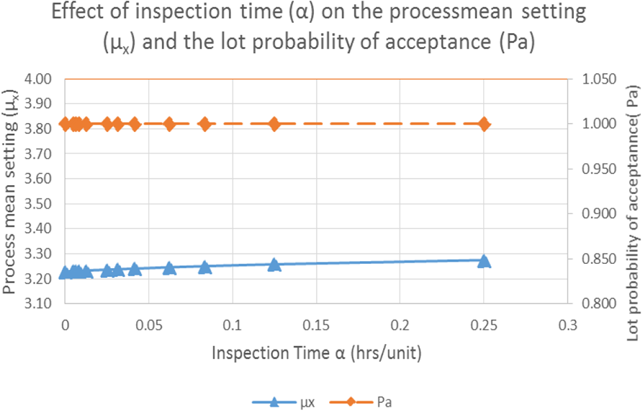
Sampling plans should be designed adequately to have sufficient segregation power when incoming lots’ quality deteriorates. Three different sampling plans are considered, each of which has the same sample size but different acceptance limits. The sample size used is fixed ( n = 89), whereas the acceptance limits are c = 2, 4 or 6. The three sampling plans are denoted as tightened (c = 2), moderate (c = 4) and relaxed (c = 6). For each sampling plan, the inspection time per unit (α) is changed and their impact on the model’s performance is monitored. Figures 2 –7 show the results of varying the inspection time on the model decision variables under various types of sampling plans.

Figure 2.
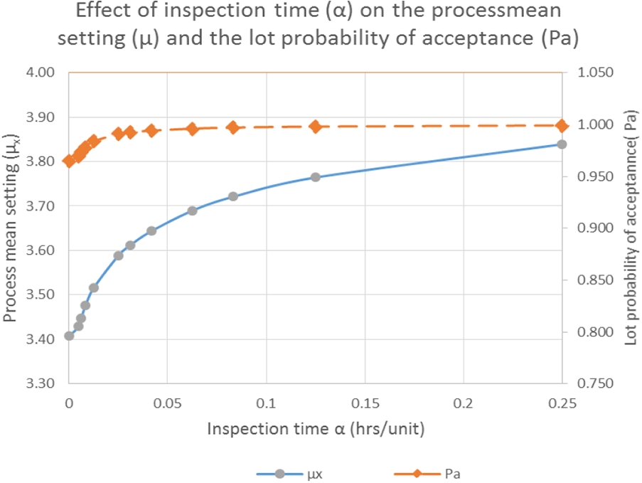
Effect of inspection time (α) on the process mean setting (µ) and lot probability of acceptance (Pa) under the tightened sampling plan.

Figure 3.
Effect of inspection time (α) on the reorder level (R) and order quantity (Q) under the tightened sampling plan.

Figure 4.
Effect of inspection time (α) on the process mean setting (µ_x) and lot probability of acceptance (Pa) under the moderate sampling plan.

Figure 5.
Effect of inspection time (α) on the reorder level (R) and order quantity (Q) under the moderate sampling plan.

Figure 6.
Effect of inspection time (α) on the process mean setting (µ) and lot probability of acceptance (Pa) under the relaxed sampling plan.

Figure 7.
Effect of inspection time (α) on the reorder level (R) and order quantity (Q) under the relaxed sampling plan.

Figures 2 and 3 show the effect of varying the inspection time under tightened sampling plan. Figure (2) shows that, as α increases, the process mean setting ( $µ_{x}$ ) will increase to reduce the effects of the extended lead-time period related costs. This increase in $µ_{x}$ leads to an increase in the probability of acceptance (Pa). It is clear that the increase in inspection time made $µ_{x}$ increase over the range of [3.41, 3.84]. This increase in $µ_{x}$ values is attributed to the effect of the tightened sampling plan, The effects of the inspection time over Q and R is almost negligible as seen by Figure 3.

The same behavior has been reported under the moderate sampling plan. Again, as can be seen in Figure 4, the increase in the inspection time is accompanied by the increase of both $µ_{x}$ and Pa. This increase is explained by the need to reduce the effects of the extended lead-time period related costs. In contrast to Figure 2, the variation of $µ_{x}$ was limited to fall over a smaller range of [3.26, 3.46]. This demonstrates how $µ_{x}$ can adapt to reduce the effects of inspection time under moderate sampling plans. The effects of the inspection time over Q and R is almost negligible as shown in Figure 5.

Figures 6 and 7 show the effect of inspection time for the relaxed sampling plan. In this case, the inspection duration (α > 0) has no effect on $µ_{x}$ , Q, or R. The process mean setting $µ_{x}$ is almost set at 3.23, with minor upward deviations ensuring a 100% acceptance level (Pa = 1.00 at three significance levels).

Figure 8 shows the effect of inspection time over total cost under the three sampling plans. It is clear that, under the relaxed sampling plan, the inspection time has no effect on the total cost, and the total cost is the least among the three modes. In contrast, whenever the sampling plan is more tightened, as for the moderate and tightened plans, the total cost becomes higher.

Figure 8.
Effect of inspection time on the total cost under various sampling plans.

The effect of the inspection time over Q, and R under different sampling plans is negligible. The values of Q and R did not vary that much. It was almost fixed at 1140, 495 with some variation around these levels.

Effects of the main cost parameters

In this section, we use a moderate sampling plan (n = 89, c = 4) throughout the analysis. Tables 1–3 show the effects of the main cost parameters $C_{d}$ C_r and C on the decision variables of the model. Table 1 presents the effect of $C_{d}$ . As seen by Table 1, the effect of C_d over Q, and R is negligible. Different values of C_d has been used with different inspection times and yet the values of Q and R were almost stable at 1140, and 480 with minor fluctuations. The effect of C_d over $µ_{x}$ and the total cost is clear. As C_d increases, and as α increases too, $µ_{x}$ will increase leading to an increase in the total cost.

Table 1.
Effect of the variation of Cd on the main cost parameters over various inspection times.

Sampling Plan n = 89 c = 4

µ_x R Q TC Pa

Cd = 10 0 3.07 487.63 1153.80 174,430 0.971

0.008 3.12 504.69 1135.10 176,160 0.982

0.025 3.21 491.34 1105.10 179,100 0.993

0.050 3.27 482.01 1128.70 181,150 0.996

0.125 3.35 484.88 1143.40 183,960 0.998

0.250 3.41 485.93 1148.00 186,140 0.999

Cd = 30 0 3.26 487.49 1153.50 189,750 0.996

0.008 3.28 482.01 1130.60 190,100 0.997

0.025 3.33 483.66 1139.10 190,780 0.998

0.050 3.36 484.82 1143.80 191,430 0.999

0.125 3.41 485.68 1147.40 192,570 0.999

0.250 3.46 486.01 1149.10 193,630 1.000

Cd = 50 0 3.45 487.73 1154.00 198,970 1.000

0.008 3.45 485.90 1148.70 199,010 1.000

0.025 3.46 486.00 1149.10 199,120 1.000

0.050 3.48 485.87 1148.90 199,260 1.000

0.125 3.50 486.17 1149.90 199,590 1.000

0.25 3.53 486.24 1150.2 200,000 1.000

Pa: is the Probability of accepting incoming lots.

Table 2.
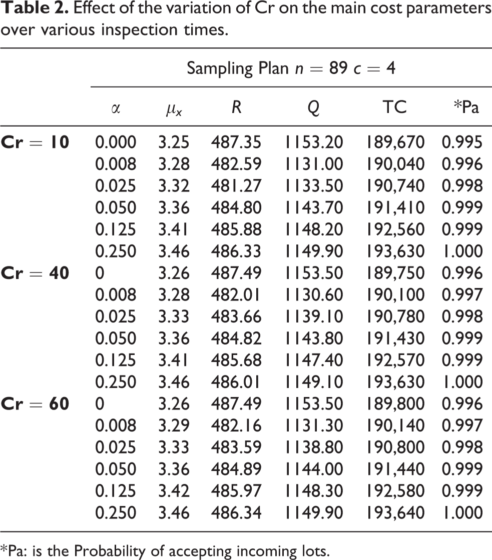
Effect of the variation of Cr on the main cost parameters over various inspection times.

Sampling Plan n = 89 c = 4

α µ_x R Q TC Pa

Cr = 10 0.000 3.25 487.35 1153.20 189,670 0.995

0.008 3.28 482.59 1131.00 190,040 0.996

0.025 3.32 481.27 1133.50 190,740 0.998

0.050 3.36 484.80 1143.70 191,410 0.999

0.125 3.41 485.88 1148.20 192,560 0.999

0.250 3.46 486.33 1149.90 193,630 1.000

Cr = 40 0 3.26 487.49 1153.50 189,750 0.996

0.008 3.28 482.01 1130.60 190,100 0.997

0.025 3.33 483.66 1139.10 190,780 0.998

0.050 3.36 484.82 1143.80 191,430 0.999

0.125 3.41 485.68 1147.40 192,570 0.999

0.250 3.46 486.01 1149.10 193,630 1.000

Cr = 60 0 3.26 487.49 1153.50 189,800 0.996

0.008 3.29 482.16 1131.30 190,140 0.997

0.025 3.33 483.59 1138.80 190,800 0.998

0.050 3.36 484.89 1144.00 191,440 0.999

0.125 3.42 485.97 1148.30 192,580 0.999

0.250 3.46 486.34 1149.90 193,640 1.000

Pa: is the Probability of accepting incoming lots.

Table 3.
Effect of the variation of the material cost per unit ( C ) on the main cost parameters over various inspection times.

Sampling Plan n = 89 c = 4

µ R Q TC Pa

C = 0.5 0.000 3.52 487.45 1153.40 105,390 1.000

0.008 3.53 486.20 1150.10 105,410 1.000

0.025 3.53 486.08 1149.90 105,460 1.000

0.050 3.55 486.23 1150.30 105,530 1.000

0.125 3.57 486.17 1150.10 105,680 1.000

0.250 3.59 486.54 1151.10 105,860 1.000

C = 1 0 3.26 487.49 1153.50 189,750 0.996

0.008 3.28 482.01 1130.60 190,100 0.997

0.025 3.33 483.66 1139.10 190,780 0.998

0.050 3.36 484.82 1143.80 191,430 0.999

0.125 3.41 485.68 1147.40 192,570 0.999

0.250 3.46 486.01 1149.10 193,630 1.000

C = 1.5 0 3.13 487.45 1153.40 269,450 0.983

0.008 3.16 504.17 1133.90 270,390 0.987

0.025 3.22 488.62 1099.00 272,440 0.994

0.050 3.27 482.19 1129.50 274,110 0.996

0.125 3.34 484.92 1143.00 276,710 0.998

0.250 3.39 485.89 1147.50 278,930 0.999

Pa: is the Probability of accepting incoming lots.

As shown in Table 2, changing C_r over three different values (10, 40, 60) had no effect on the model performance. The same results were evident at various inspection times. Recall that this experiment was conducted while other parameters were kept at their base levels. More specifically, $C_{d} = 30$ and $C = 1$ . This shows that both $C_{d}$ and C have more effect than $C_{r}$ . If $C_{d} = 30$ and $C = 1$ , the probability of acceptance is always beyond 0.995, leaving negligible chance for C_r to be active. This explains the behavior seen in Table 2.

Table 3 shows the effect of the variation of the material cost per unit (C) on the model performance. It is clear that the behavior of varying C is almost the reverse compared with C_d . When C = 0.5, as α increases, $µ_{x}$ will range between 3.52 and 3.59, At C = 1.0, and as α increases, $µ_{x}$ ranges between 3.26 and 3.46. At C = 1.5, and as α increases, $µ_{x}$ will change from 3.13 to 3.39. In general, higher material cost will restrict the ability of $µ_{x}$ to assume higher values since higher costs will be incurred. But as α increases, $µ_{x}$ will increase too leading to higher material/total costs. Again the effect of C on Q and R is also negligible. The values of Q and R are also stable at 1140, 480 with some variations.

In this example, the effects of sampling plans, inspection time, C, C_d , and C_r shows minor effect over Q, and $R$ values. However, their impact is clear over process mean setting $µ_{x}$ and the total cost of the model.

Discussion and conclusion

This paper presented a study on the effect of sampling inspection for a two-stage supply chain model that involves a producer and a distributer. The major contribution here is addressing a two-echelon supply chain involving a producer and distributer with sampling inspection. The distributer’s warehouse was controlled by a $Q - R$ system. Relaxed assumptions were made for negligible inspection time. Two cases of inspection were addressed; (1) sampling inspection for dispatched lots, and (2) 100% inspection for rejected lots. For the latter case, the time any lot spends under 100% inspection is not negligible, and it was assumed to be proportional to the lot size Q. Furthermore, the lead time duration had to be extended to account for the 100% inspection time. The developed cost model is helpful to find the optimal values of the production process mean ( $µ_{x}$ ), and simultaneously, determines the proper setting of the order quantity (Q) and reorder level (R), under a given sampling plan with non-negligible 100% inspection time.

In practice, sampling is still a viable alternative and in some scenarios, it is the only method that can be used to ensure the quality of incoming lots. Hence, sampling parameters can have large impact on the supply chain performance (especially the inspection time). For instance, whenever the inspection time is high, the supply chain will incur additional losses related to the extended lead-time period. To reduce the effects of these losses, the producer will need to improve the quality of his production (i.e., larger value of $µ_{x}$ in our model). The same effect was observed for both C_d and C_r . Yet, the material cost per unit, C, restricts the ability of the producer to improve the quality (i.e. larger value of $µ_{x}$ ). The type of sampling plans was also found to have a significant effect on the performance of the supply chain. Even though they have the largest segregation power, adopting a tightened sampling plans is not always the best policy for the considered supply chain. In this case, the producer is forced to adding extra material to avoid lots rejection. Therefore, higher total cost by the supply chain will be incurred. A similar analogy can be made for either moderate, or relaxed sampling policies. We believe that the best policy is not a specific one of the three presented modes. A dynamic sampling policy that uses a combination of them with the proper design of the switching rule will be more suitable. Proper determination of the switching rules between tightened, moderate and relaxed sampling plans will offer a strong, flexible sampling policy that considers producers’ commitment to quality and adopts for quality variations of incoming lots. At the same time, it balances the trade-offs among the relevant cost parameters. We believe that this could be an interesting topic for future research.

	Sampling Plan n = 89 c = 4
Cd = 10	0	3.07	487.63	1153.80	174,430	0.971
0.008	3.12	504.69	1135.10	176,160	0.982
0.025	3.21	491.34	1105.10	179,100	0.993
0.050	3.27	482.01	1128.70	181,150	0.996
0.125	3.35	484.88	1143.40	183,960	0.998
0.250	3.41	485.93	1148.00	186,140	0.999
Cd = 30	0	3.26	487.49	1153.50	189,750	0.996
0.008	3.28	482.01	1130.60	190,100	0.997
0.025	3.33	483.66	1139.10	190,780	0.998
0.050	3.36	484.82	1143.80	191,430	0.999
0.125	3.41	485.68	1147.40	192,570	0.999
0.250	3.46	486.01	1149.10	193,630	1.000
Cd = 50	0	3.45	487.73	1154.00	198,970	1.000
0.008	3.45	485.90	1148.70	199,010	1.000
0.025	3.46	486.00	1149.10	199,120	1.000
0.050	3.48	485.87	1148.90	199,260	1.000
0.125	3.50	486.17	1149.90	199,590	1.000
0.25	3.53	486.24	1150.2	200,000	1.000

	Sampling Plan n = 89 c = 4
Cr = 10	0.000	3.25	487.35	1153.20	189,670	0.995
0.008	3.28	482.59	1131.00	190,040	0.996
0.025	3.32	481.27	1133.50	190,740	0.998
0.050	3.36	484.80	1143.70	191,410	0.999
0.125	3.41	485.88	1148.20	192,560	0.999
0.250	3.46	486.33	1149.90	193,630	1.000
Cr = 40	0	3.26	487.49	1153.50	189,750	0.996
0.008	3.28	482.01	1130.60	190,100	0.997
0.025	3.33	483.66	1139.10	190,780	0.998
0.050	3.36	484.82	1143.80	191,430	0.999
0.125	3.41	485.68	1147.40	192,570	0.999
0.250	3.46	486.01	1149.10	193,630	1.000
Cr = 60	0	3.26	487.49	1153.50	189,800	0.996
0.008	3.29	482.16	1131.30	190,140	0.997
0.025	3.33	483.59	1138.80	190,800	0.998
0.050	3.36	484.89	1144.00	191,440	0.999
0.125	3.42	485.97	1148.30	192,580	0.999
0.250	3.46	486.34	1149.90	193,640	1.000

	Sampling Plan n = 89 c = 4
C = 0.5	0.000	3.52	487.45	1153.40	105,390	1.000
0.008	3.53	486.20	1150.10	105,410	1.000
0.025	3.53	486.08	1149.90	105,460	1.000
0.050	3.55	486.23	1150.30	105,530	1.000
0.125	3.57	486.17	1150.10	105,680	1.000
0.250	3.59	486.54	1151.10	105,860	1.000
C = 1	0	3.26	487.49	1153.50	189,750	0.996
0.008	3.28	482.01	1130.60	190,100	0.997
0.025	3.33	483.66	1139.10	190,780	0.998
0.050	3.36	484.82	1143.80	191,430	0.999
0.125	3.41	485.68	1147.40	192,570	0.999
0.250	3.46	486.01	1149.10	193,630	1.000
C = 1.5	0	3.13	487.45	1153.40	269,450	0.983
0.008	3.16	504.17	1133.90	270,390	0.987
0.025	3.22	488.62	1099.00	272,440	0.994
0.050	3.27	482.19	1129.50	274,110	0.996
0.125	3.34	484.92	1143.00	276,710	0.998
0.250	3.39	485.89	1147.50	278,930	0.999

Footnotes

Declaration of conflicting interests

The author(s) declared no potential conflicts of interest with respect to the research, authorship, and/or publication of this article.

Funding

The author(s) disclosed receipt of the following financial support for the research, authorship, and/or publication of this article: The authors would like to acknowledge the support provided by King Fahd University of Petroleum & Minerals, Dhahran, Saudi Arabia (grant #SB181035).

ORCID iD

Mohammad M AlDurgam

References

Simchi-Levi

Kaminsky

Simchi-Levi

. Designing and managing the supply chain: concepts, strategies, and case studies. 3rd edn. Boston: McGraw-Hill/Irwin, 2008.

Rahim

Ben-Daya

. Integrated models in production planning, inventory, quality, and maintenance. Berlin: Springer US, 2001.

AlDurgam

. Dynamic maintenance, production and inspection policies, for a single-stage, multi-state production system. IEEE Access 2020; 8: 105645–105658.

Goyal

. An integrated inventory model for a single supplier–single customer problem. Int J Prod Res 1977; 15: 107–111.

Glock

. The joint economic lot size problem: a review. Int J Prod Econ 2012; 135: 671–686.

Darwish

Abdulmalek

. An integrated single-vendor single-buyer targeting problem with time-dependent process mean. IJLSM 2012; 13: 51.

Darwish

Abdulmalek

Alkhedher

. Optimal selection of process mean for a stochastic inventory model. Eur J Oper Res 2013; 226: 481–490.

Hunter

Kartha

. Determining the most profitable target value for a production process. J Qual Technol 1977; 9: 176–181.

Chen

. Optimal process mean and standard deviation settings for rectifying sampling inspection plan with quality investment. J Stat Manag Syst 2019; 22: 893–899.

10.

Gong

Roan

Tang

. Process mean determination with quantity discounts in raw material cost. Decis Sci 1998; 29: 271–302.

11.

Al-Fawzan

Hariga

. An integrated inventory-targeting problem with time-dependent process mean. Prod Plan Control 2002; 13: 11–16.

12.

Hariga

Al-Fawzan

. Joint determination of target value and production run for a process with multiple markets. Int J Prod Econ 2005; 96: 201–212.

13.

Darwish

. Economic selection of process mean for single-vendor single-buyer supply chain. Eur J Oper Res 2009; 199: 162–169.

14.

Alkhedher

Darwish

. Optimal process mean for a stochastic inventory model under service level constraint. IJOR 2013; 18: 346.

15.

Darwish

Aldaihani

. Economic selection of process mean and lot-sizing decisions for multi-newsvendor supply chain. Int Trans Oper Res 2015; 22: 1055–1070.

16.

Uthayakumar

Rameswari

. An integrated inventory model for a single vendor and single buyer with order-processing cost reduction and process mean. Int J Prod Res 2012; 50: 2910–2924.

17.

Raza

Turiac

. Joint optimal determination of process mean, production quantity, pricing, and market segmentation with demand leakage. Eur J Oper Res 2016; 249: 312–326.

18.

Lee

Rosenblatt

. Optimal inspection and ordering policies for products with imperfect quality. IIE Trans 1985; 17: 284–289.

19.

Zhang

Gerchak

. Joint lot sizing and inspection policy in an EOQ model with random yield. IIE Trans 1990; 22: 41–47.

20.

Peters

Schneider

Tang

. Joint determination of optimal inventory and quality control policy. Manag Sci 1988; 34: 991–1004.

21.

Salameh

Jaber

. Economic production quantity model for items with imperfect quality. Int J Prod Econ 2000; 64: 59–64.

22.

Goyal

Cárdenas-Barrón

LE.

Note on: economic production quantity model for items with imperfect quality—a practical approach. Int J Prod Econ 2002; 77: 85–87.

23.

AlDurgam

Selim

Al-Shihabi

, et al. Economic production quantity model with variable machining rates and product quality. Int J Eng Bus Manag 2019; 11: 184797901987261.

24.

Cheung

Leung

. Coordinating replenishments in a supply chain with quality control considerations. Prod Plan Control 2000; 11: 697–705.

25.

Ben-Daya

Noman

Hariga

. Integrated inventory control and inspection policies with deterministic demand. Comput Oper Res 2006; 33: 1625–1638.

26.

Ouyang

. Integrated vendor–buyer inventory system with sublot sampling inspection policy and controllable lead time. Int J Syst Sci 2007; 38: 339–350.

27.

Hsieh

Liu

. Quality investment and inspection policy in a supplier–manufacturer supply chain. Eur J Oper Res 2010; 202: 717–729.

28.

Sharifi

Hasanpour

Taleizadeh

. A lot sizing model for imperfect and deteriorating product with destructive testing and inspection errors. Int J Syst Sci 2019; 1–12. DOI: 10.1080/23302674.2019.1648702.

29.

Bouslah

Gharbi

Pellerin

. Joint optimal lot sizing and production control policy in an unreliable and imperfect manufacturing system. Int J Prod Econ 2013; 144: 143–156.

30.

Duffuaa

El-Ga’aly

. A multi-objective optimization model for process targeting using sampling plans. Comput Ind Eng 2013; 64: 309–317.

31.

Duffuaa

El-Ga’aly

. A multi-objective mathematical optimization model for process targeting using 100% inspection policy. Appl Math Model 2013; 37: 1545–1552.

32.

Duffuaa

El-Ga’aly

. A multi-objective optimization model for process targeting with inspection errors using 100% inspection. Int J Adv Manuf Technol 2017; 88: 2679–2692.

33.

Chen

Chou

Kan

. Economic specification limits and process mean settings by considering unequal target value and specification center. J Ind Prod Eng 2014; 31: 199–205.

34.

Ben-Daya

Noman

. Integrated inventory and inspection policies for stochastic demand. Eur J Oper Res 2008; 185: 159–169.

35.

Al-Sultan

Pulak

MFS

. Optimum target values for two machines in series with 100% inspection. Eur J Oper Res 2000; 120: 181–189.

36.

Shao

Fowler

Runger

. Determining the optimal target for a process with multiple markets and variable holding costs. Int J Prod Econ 2000; 65: 229–242.

	Sampling Plan n = 89 c = 4
		µ_x	R	Q	TC	*Pa
Cd = 10	0	3.07	487.63	1153.80	174,430	0.971
	0.008	3.12	504.69	1135.10	176,160	0.982
	0.025	3.21	491.34	1105.10	179,100	0.993
	0.050	3.27	482.01	1128.70	181,150	0.996
	0.125	3.35	484.88	1143.40	183,960	0.998
	0.250	3.41	485.93	1148.00	186,140	0.999
Cd = 30	0	3.26	487.49	1153.50	189,750	0.996
	0.008	3.28	482.01	1130.60	190,100	0.997
	0.025	3.33	483.66	1139.10	190,780	0.998
	0.050	3.36	484.82	1143.80	191,430	0.999
	0.125	3.41	485.68	1147.40	192,570	0.999
	0.250	3.46	486.01	1149.10	193,630	1.000
Cd = 50	0	3.45	487.73	1154.00	198,970	1.000
	0.008	3.45	485.90	1148.70	199,010	1.000
	0.025	3.46	486.00	1149.10	199,120	1.000
	0.050	3.48	485.87	1148.90	199,260	1.000
	0.125	3.50	486.17	1149.90	199,590	1.000
	0.25	3.53	486.24	1150.2	200,000	1.000

An integrated process targeting and continuous review system with sampling inspection

Abstract

Keywords

Introduction

Literature review

Integrated process targeting and inventory control models

Integrated inventory and inspection sampling models

Synthesis of both research streams

Model assumptions and notations

The effect of sampling inspection

Lemma

Proof

Case 1: If the lot is accepted

Case 2: If the lot is rejected

The effect of sampling inspection on the received lot size Q

The effect on the safety stock level(s)

The effect of sampling inspection on the inventory cycle time

Model development

Model analysis and solution procedure

Numerical results

Quality sampling plan and inspection time

Effects of the main cost parameters

Discussion and conclusion

Footnotes

Declaration of conflicting interests

Funding

ORCID iD

References