Sage Journals: Discover world-class research

Abstract

Construction cost index has been widely used to prepare cost estimates, budgets, and bids for construction projects. It can also be regarded as an indicator of cost level, which makes it valuable to public authorities for understanding the conditions in the construction industry. Accurate forecasting of future construction cost index is essential for construction industry at both micro- and macro-level. To improve the accuracy of the cost forecasting, time series modeling techniques are adopted in this study. The performance of the exponential smoothing models and seasonal autoregressive integrated moving average (ARIMA) models for forecasting the building cost of five categories of residential building (one-story house, two-story house, town house, apartment, and retirement village building) in New Zealand is compared. Exponential smoothing models can produce more accurate forecasts for cost series of the one-story house and two-story house in New Zealand, while seasonal ARIMA models outperform exponential smoothing models across the cost series for town house, apartment, and retirement village building. This study contributes toward the development of the current state of knowledge in the area of cost index forecasting for New Zealand and provides insights that should be valuable from the practitioner perspectives.

Keywords

Residential building costs exponential smoothing model ARIMA model forecasting performance New Zealand

Introduction

Construction cost index has been widely used in construction cost estimate preparation, bid and budget preparation, and cost control and risk management.^1

–4 Accurate cost estimates can lead to more reliable bids and help to achieve goals since reliable and reasonable cost forecasting can improve business strategy. Over the past few decades, many projects have suffered huge losses due to the considerable difference between the final project cost and the initial cost estimate.⁵ Several studies found that changes in construction cost is one of the most critical risks that affect the project budget and profit.^6
–8 Moreover, contractors may suffer high cost variation, insufficient cash flow, and delayed progress associated with the high variation of cost index. Although cost index increases in the long term, it has short-term variations, which makes it difficult to obtain accurate cost estimates.

The construction industry is essential to New Zealand’s economy, contributing significantly to business, GDP, and employment.⁹ The construction industry is highly integrated across the economy and uses outputs from a number of key industries across New Zealand.⁹ This integration means that the construction industry can significantly influence other industries of New Zealand’s economy. It is an important sector and its economic performance and productivity plays an important role in the overall health of the economy.¹⁰ Economic growth is reliant on contributions from the construction industry. However, the construction industry is a resource-based sector. If the sector consumes an excessive amount of unrecoverable natural resources, they will cost more in the future. Monitoring the construction industry and proper allocation of resources are essential to long-term economic development. Given the importance of this industry to the overall economy, proper monitoring of the industry is essential to policy makers and strategy developers at the industry and national levels.¹¹ However, identifying an appropriate indicator for monitoring the construction industry is difficult. Some studies suggest that productivity may be a qualified indicator of the construction industry. However, according to Harrison¹² and Rojas and Aramvareekul,¹³ productivity is an inaccurate indicator of the construction industry since errors exist in the measurements and calculations. Also, Sui¹⁴ used quality to measure the construction industry; however, quality is a qualitative indicator that needs other quantified factors to measure it.

Cost index is an effective tool for capturing trends and provides insight into understanding complex and dynamic environments.¹⁵ Cost index reflects the unit price of basic materials, which is a good indicator for comparing the input and output. Moreover, compared with economic indicators that only reflect the economic activities in the construction industry,¹¹ construction cost index also incorporates other factors such as the relationship between demand and supply. Cost index forecasts can help the government to plan its investment in order to smooth the boom–bust cycle inherent to the construction industry. For example, countercyclical investment by the government may reduce volatility in the industry and reduce the magnitude of busts. Better planning can guarantee certainty of work and better resource planning in the industry, improving industry performance and productivity.

Given the utmost importance of cost forecasting and the important role of predicting it accurately, this study tends to use time series modeling techniques to forecast the building cost of five categories of residential building (one-story house, two-story house, town house, apartment, and retirement village building) in New Zealand. Building costs time series usually exhibit strong trends presenting challenges in developing useful models. How to effectively model building cost series and how to enhance forecasting performance are still outstanding questions. There are two most widely used time series forecasting methods: exponential smoothing and autoregressive integrated moving average (ARIMA). The performance of the two forecasting techniques was evaluated in terms of error measures.

Exponential smoothing method was originally introduced by Holt,¹⁶ Brown,¹⁷ and Winters¹⁸ for short-term sales forecasting in support of supply chain management and production planning. The widespread usage of this method is mainly due to the fact that it is a relatively simple forecasting method requiring a small-sized sample and having a comprehensible statistical framework and model parameters. Exponential smoothing models developed are based on the trend and seasonality in time series, while ARIMA models are supposed to describe the autocorrelations in the time series. A framework for exponential smoothing methods was developed based on state-space models.¹⁹

ARIMA approach is a renowned and widely used linear method.²⁰ It carries more flexibility by representing various components of time series including autoregressive (AR), moving average (MA), and combined AR and MA. ARIMA can model the underlying changes in cost data to make structural forecasts.²¹ It is the most efficient approach for short-term forecasting with rapid changes. ARIMA models can also predict the future based on modeling the behavior of the serial correlation between the observations of the time series. The future predictions based on ARIMA models can be explained by previous or lagged values and the terms of the stochastic errors.²²

Time series forecasting techniques such as exponential smoothing models and the ARIMA models have not yet been examined for residential building cost forecasting in New Zealand. Therefore, the study as original contribution to the existing literature is for the first time to evaluate the forecasting performance of these models for residential building cost in New Zealand. Moreover, based on the comparison of the forecasting techniques, industry practitioners can obtain a general understanding of forecasting techniques for building cost, and thereby improve forecasting accuracy.

The rest of this study is organized as follows. The second section presents the previous related works about forecasting methods for construction cost index. The third section illustrates exponential smoothing method and ARIMA models in detail. Both exponential smoothening and ARIMA models for the cost series of New Zealand are shown in the fourth section. In the fifth section, forecasting performance of the proposed models is compared based on error measures. Discussion of the results is presented in the sixth section. In the final section, conclusion is presented.

Research background

Two of the most widely used forecasting models for construction cost index were published in previous works: the causal method and the time series method.^5,21,23 Causal methods usually adopt regression models to estimate construction costs. Trost and Oberlender²⁴ introduced a mathematical model for investigating the accuracy of early cost estimates by using principal component analysis and regression analysis. Ng et al.²⁵ introduced an integrated regression analysis and ARIMA techniques to predict a tender price index for Hong Kong building projects. Moreover, Hwang²⁶ used dynamic model that includes past values of cost index and explanatory variables to forecast construction cost index of the United States. Hwang and Liu²⁷ addressed a dynamic regression model to examine the relationship between the economic conditions in the market and construction cost. Although these methods are effective by incorporating the explanatory variables to obtain accurate cost estimates, they are difficult to deal with as time-varying variables and reflect the time lag effects. Since much time-related variables have an autocorrelation,²⁸ time-related techniques can be adopted to overcome these limitations.

In an attempt to solve time-related problems in the methods, time series techniques, which estimate future values of a certain variable according to past values of itself and random shock factors, have been adapted to cost forecasting in construction projects. For example, Fellows²⁹ used time series models to provide reliable forecasts of building costs, tender prices, and the impacts of economic inflation on building projects. According to Wong et al.,³⁰ it is possible to make accurate predications based on historical patterns. Several studies have been conducted using the time series method. For example, Ashuri and Lu²¹ illustrated a time series method that estimates future values according to past values and corresponding random errors and produces a reliable prediction of construction cost. These time series techniques provide systematic and time-related models to forecast future values. Hwang² used a time series model to estimate the construction cost index. Xu and Moon⁴ employed a vector model to forecast construction cost trends.

Certain artificial intelligence (AI) methods were used to forecast the construction cost index. For example, Williams³¹ explained a way of applying neutral networks to forecast changes in the construction cost index. Kim et al.³² used three forecasting methods to estimate construction cost index including multiple regression analysis, neutral networks, and case-based reasoning. Cheng et al.³³ developed a hybrid model, the evolutionary least square support vector machine, to forecast the Taiwanese construction cost index. The results indicated that an AI method can be used as an effective method for forecasting the Taiwanese construction cost index. Also, Cao et al.³⁴ used a hybrid computation model that included multivariate adaptive regression splines, a radial basis function neutral network, and an artificial bee colony to forecast the Taiwanese construction cost index.

The forecasting methods described above generate accurate forecasts of the construction cost index. However, there are no studies that provide an effective tool for forecasting the construction cost index of New Zealand. This study provides time series models that can model the characteristics of the construction cost index of New Zealand and generate accurate cost forecast. Although many factors can impact the construction cost,³⁵ one of the main contributors to cost fluctuation is the prices changes in construction resources such as materials, labor, and equipment.^4,36
–38

Research methods

Data

The building cost index is useful for construction professionals to quantify cost variations.³⁹ The index can provide information of cost changes caused by a combination of changes in material, labor, and equipment.²⁷ Hence, the cost index has been used widely in the industry for cost estimation.³ The cost index provided by QV costbuilder has been accepted in the Architectural, Engineering and Construction (AEC) industry in New Zealand. Since 2000, QV has published construction cost index for four major cities of New Zealand. For more information about the construction cost index, readers can refer to the QV website.⁴⁰ The construction cost index includes costs among a wide range of materials and buildings. QV costbuilder carried out various surveys on construction economics including construction material, labor, and equipment costs to provide comprehensive statistical information. As for many other industries and sectors, QV costbuilder compiles historical data to guide construction organizations and industry professionals and to identify cost fluctuations in the construction industry.

This study uses quarterly CCI for the period of first quarter 2001 to the fourth quarter 2018. The available data set consists of quarterly cost data over a period of 18 years (72 observations) for five categories of residential buildings in New Zealand. It is usual to separate the data into two sections: in-sample data and out-of-sample data. The in-sample data are used for model fitting and the out-of-sample data aim to evaluate the forecasting performance of the model.⁴¹ The data (72 observations) were split into two parts: the training part for model fitting and the testing part for evaluating forecasting performance by comparing forecasts with observations.⁴² There is no clear rule for this dividing; in this study, about 72% of the data (2001: Q1–2013: Q4) were used for model fitting and the remaining 28% (2014: Q1–2018: Q4) were used for out-of-sample forecasts evaluation. The quarterly average building cost for the five categories of residential building in New Zealand from 2001: Q1 to 2018: Q4 are depicted in Figure 1.

Figure 1.

Building cost time series for five categories of residential building in New Zealand.

Exponential smoothing model

Exponential smoothing is one of the most effective forecasting methods when a time series has a trend that has changed over time, for example, since the 1950s.⁴³ It unequally weights the observed time series values. More recently observed values are weighted more heavily than more remote observations. The weights for the observed time series values decrease exponentially as one moves further into the remote. A smoothing constant can determine the rate at which the weights of older observed values decrease. Exponential smoothing techniques include simple exponential smoothing, linear trend corrected exponential smoothing, Holt–Winters methods, and damped trend exponential smoothing.⁴³

According to Hyndman et al.,⁴⁴ exponential smoothing models have been widely used in many research fields and industry practices due to their relative simplicity and good overall forecasting performance as well as considering trends, seasonality, and other features of the data. A large number of existing research and studies also indicated their extensive industrial applications.^45,46 In this study, Holt–Winters exponential smoothing method was adopted.

Holt–Winters method

Holt–Winters method can be applied to time series data displaying trend and seasonality; it has level and trend smoothing parameters (α and β) in addition to a seasonal parameter (γ). Although there is no strong evidence for seasonality in the time series of the residential building costs in New Zealand, Holt–Winters method is used to evaluate whether the involvement of a seasonal parameter can improve the model. Holt–Winters methods are designed for time series that exhibit linear trend and seasonal variation, which include additive Holt–Winters method and multiplicative Holt–Winters methods.⁴³ An advantage of these methods is that they can model data seasonality directly instead of stationary transforming for the data. If a time series has a linear trend and additive seasonal pattern, the additive Holt–Winters method is appropriate. Then the time series can be described in equation (1)

Y_{t} = (β_{0} + β_{1} t) + S_{t} + ϵ_{t}

where β ₁ is growth rate, S_t is a seasonal pattern, and $ϵ_{t}$ is error term.

For such time series, the mean, the growth rate, and the seasonal variation may be changing over time. A state-space model for these changing components can be found in equations (2) to (5)

l_{t} = l_{t - 1} + b_{t - 1} + α [Y_{t} - (l_{t - 1} + b_{t - 1} + S_{t - L})]

b_{t} = b_{t - 1} + b_{t - 1} + α γ [Y_{t} - (l_{t - 1} + b_{t - 1} + S_{t - L})]

S_{t} = S_{t - L} + (1 - α) δ [Y_{t} - (l_{t - 1} + b_{t - 1} + S_{t - L})]

{\hat{Y}}_{t} = l_{t - 1} + b_{t - 1} + S_{t - L}

To begin the estimation, the initial values for level, growth rate, and seasonal variation should be estimated. Hence, first, a least squares regression model should be generated based on available data. The regression model can be expressed in equation (6). The initial values l ₀, b ₀ were also obtained from the model

{\hat{Y}}_{t} = l_{0} + b_{0} t

Obtain estimated values for each time period based on the above regression model. The initial seasonal factor in each of L seasons can be calculated in equation (7)

S_{L i} = \frac{(y_{i} - {\hat{y}}_{i}) + (y_{i + L} - {\hat{y}}_{i + L}) + (y_{i + 2 L} - {\hat{y}}_{i + 2 L}) + \dots + (y_{i + n L} - {\hat{y}}_{i + n L})}{L}

where $S_{L i}$ are seasonal factors, L is the number of seasons in a year, and i is the number of time periods in each season.

After finding the values for the seasonal factors, the state-space models are employed to obtain model parameters that minimize the sum of the squared errors. Future values of the time series are predicted by the state-space model in equation (5).

Multiplicative Holt–Winters method

If a time series has a linear trend with multiplicative seasonal variations, the multiplicative Holt–Winters is appropriate to be used. The state-space models for this method can be described in equations (8) to (11)

l_{t} = l_{t - 1} + b_{t - 1} + α \frac{[Y_{t} - (l_{t - 1} + b_{t - 1}) S_{t - L}]}{S_{t - L}}

b_{t} = b_{t - 1} + α γ \frac{[Y_{t} - (l_{t - 1} + b_{t - 1}) S_{t - L}]}{S_{t - L}}

S_{t} = S_{t - L} + (1 - α) δ \frac{[Y_{t} - (l_{t - 1} + b_{t - 1}) S_{t - L}]}{l_{t}}

Y_{t} = (l_{t - 1} + b_{t - 1}) S_{t - L}

And the seasonal factors can be computed in the following equation (12)

S_{L i} = \frac{(y_{i} / {\hat{y}}_{i}) + (y_{i + L} / {\hat{y}}_{i + L}) + (y_{i + 2 L} / {\hat{y}}_{i + 2 L}) + \dots + (y_{i + n L} / {\hat{y}}_{i + n L})}{L}

ARIMA model

There are four steps to select an appropriate model for the time series data in the Box–Jenkins approach.⁴⁷ The development process of an ARIMA model is shown in Figure 2. ARIMA models are flexible and adaptive since they can forecast data values of a time series by a linear combination of its past values, past errors (in terms of univariate analysis), and past and present values of other time series (in terms of multivariate analysis). Besides, in univariate time series analysis, the development process of ARIMA model provides a comprehensive set of tools for model identification, parameters estimation, diagnosis checking, and forecasting. Taking into account the seasonality of the time series, a seasonal ARIMA model denoted as ARIMA(p, d, q)(P, D, Q) _L is introduced, where P represents seasonal AR orders, D indicates seasonal differencing orders, Q represents seasonal MA orders, and L indicates the number of seasons.

Figure 2.

ARIMA model development process. ARIMA: autoregressive integrated moving average.

Seasonality implies that a pattern repeats itself over a fixed time interval.⁴⁸ In this study, the quarterly data present a seasonal period of four quarters. The autocorrelation function (ACF) and partial autocorrelation function (PACF) were employed to determine the stationarity in the data set. The seasonal difference was used to transform the nonstationary seasonal data into stationary by taking the difference between the current observation and the corresponding observation from the previous year. A seasonal ARIMA model can be shown in equation (13)

\emptyset_{p} (B) ϕ_{P} (B^{L}) \nabla_{L}^{D} \nabla^{d} y_{t} = δ + θ_{q} (B) ϑ_{Q} (B^{L}) a_{t}

where

\emptyset_{p} (B) = (1 - \emptyset_{1} B - \emptyset_{2} B^{2} - \dots - \emptyset_{p} B^{p})

ϕ_{P} (B^{L}) = (1 - ϕ_{1, L} B^{L} - ϕ_{2, L} B^{2 L} - \dots - ϕ_{P, L} B^{P L})

\nabla_{L}^{D} \nabla^{d} y_{t} = {(1 - B^{L})}^{D} {(1 - B)}^{d} y_{t}

θ_{q} (B) = (1 - θ_{1} B - θ_{2} B^{2} - \dots - θ_{q} B^{q})

ϑ_{Q} (B^{L}) = (1 - ϑ_{1, L} B^{L} - ϑ_{2, L} B^{2 L} - \dots - ϑ_{Q, L} B^{P L})

where B is backshift operator; L is the number of seasons in a year (L = 4 for quarterly data and L = 12 for monthly data); δ is a constant term; $a_{t}, a_{t - 1}, \dots$ are random shocks; $\emptyset_{1}, \emptyset_{2}, \dots, \emptyset_{p}$ are nonseasonal AR parameters; $ϕ_{1, L}, ϕ_{2, L}, \dots, ϕ_{P, L}$ are seasonal AR parameters; $θ_{1}, θ_{2}, \dots, θ_{q}$ are nonseasonal MA parameters; and $ϑ_{1, L}, ϑ_{2, L}, \dots, ϑ_{Q, L}$ are seasonal MA parameters.

Stationary checking

Classical ARIMA models are usually used to describe stationary time series. Thus, in order to identify an appropriate ARIMA model, the stationary of the times series should be determined at first. If the time series is not stationary, the transformation of the time series to stationary should be undertaken. A stationary time series can be described as the statistical properties (e.g. the mean and the variance) of it are essentially constant over time.⁴³ The differences of the time series values are shown in equation (16).

The parameters are usually estimated by the least square method. The least square estimation method means that the model parameters minimize the sum of the squared errors. The sum of the squared errors can be computed by using equation (19)

SSE = \sum_{t = 1}^{n} {(y_{t} - {\hat{y}}_{t})}^{2}

where y_t is the real value of the time series and ${\hat{y}}_{t}$ is the value estimated by the tentative model.

Diagnostic checking

The obtained models should be checked for whether the ARIMA assumptions are satisfied. As a more accurate test, the Ljung–Box test is usually undertaken to examine whether the autocorrelation of the residuals are statistically different from an expected white noise process. If the p value is greater than 0.05, indicating no significant autocorrelation in residuals, in turn, the model is adequate.⁴⁹

Forecasting error measure

Error measures are widely used for examining the accuracy of a forecasting model, which have many forms, including root mean square error (RMSE),⁵⁰ mean squared error (MSE),⁵¹ and mean absolute percentage error (MAPE).⁵² This study evaluated the accuracy of the forecasts by MAPE between the actual and predicted values of building cost. The lower the values are, the better the forecasting performance of the proposed model. Denote the real observations for the time series by y_i and the forecasting values for the same series by ${\hat{y}}_{i}$ . MAPE can be computed in equation (20)

MAPE = \frac{{\sum_{i = 1}^{n} | \frac{y_{i} - {\hat{y}}_{i}}{y_{i}} |}_{}^{}}{n} \times 100 %

Models for cost series

Holt–Winters models for building cost

Both additive Holt–Winters and multiplicative Holt–Winters models were applied to the five cost series. Following the methods outlined in the third section, the model parameters were estimated. The results of the exponential smoothing models for the cost of the five categories of the residential building are displayed in Table 1. The p value of the model parameters is less than 0.05, indicating that the parameters are significant and that they can remain in the model. Moreover, the model fit R ² and error measures including RMSE, MAPE, and mean absolute error (MAE) were also generated. In addition, the model parsimony measure Bayesian information criterion (BIC) was also obtained. The results are shown in Table 3. As the results show, the values of BIC for the exponential smoothing models are similar, which indicate the models are parsimonious. The error measures indicate Holt–Winters models can fit the cost series fairly well.

Table 1.

Estimated parameter values with significant test for exponential smoothing models.

Series	Exponential smoothing model	Parameter	Estimate	SE	p Value
AR1	ES (AHW)	α	0.370	0.116	0.002
		β	0.634	0.287	0.032**
		γ	0	0.112	0.993
	ES (MHW)	α	0.379	0.112	0.001**
		β	0.537	0.251	0.037**
		γ	0.528	0.171	0.003**
AR2	ES (AHW)	α	0.899	0.150	***
		β	0	0.047	1
		γ	0	0.696	1
	ES (MHW)	α	0.846	0.145	***
		β	0.001	0.045	0.983
		γ	0.028	0.298	0.925
AR3	ES (AHW)	α	0.683	0.135	***
		β	0.218	0.113	0.059*
		γ	0.001	0.171	0.995
	ES (MHW)	α	0.578	0.128	***
		β	0.269	0.128	0.042**
		γ	0.020	0.091	0.830
AR4	ES (AHW)	α	0.200	0.079	0.014**
		β	1.000	0.467	0.037**
		γ	0	0.091	1
	ES (MHW)	α	0.198	0.083	0.021**
		β	1.000	0.503	0.052*
		γ	0.040	0.062	0.524
AR5	ES (AHW)	α	0.469	0.118	***
		β	0.441	0.194	0.027**
		γ	0.014	0.096	0.883
	ES (MHW)	α	0.361	0.096	***
		β	0.511	0.225	0.028**
		γ	0.479	0.151	0.003**

AHW: additive Holt–Winters; MHW: multiplicative Holt–Winters.

***p < 0.01; **p < 0.05; *p < 0.1.

Seasonal ARIMA models

Model selection

Box et al.²⁰ suggested that to properly implement the ARIMA method a time series with at least 30 observations is required. In this study, for each cost series, a total of 52 observations from 2001: Q1 to 2013: Q4 were used to obtain the proposed models. For the stationary analysis of the five cost series, ACF and PACF were used; results are shown in Figure 3. On investigating the graphs of ACF and PACF for the five building cost series, it can be observed that the ACFs decay very slowly at both nonseasonal and seasonal lags. For each cost series, the appropriate number of differencing should be determined. Hence, it is reasonable to transform to a stationary series by taking four quarter differencing of data to remove seasonality and regular differencing to remove trends for the four cost series, except the cost series for the two-story house in New Zealand. The cost series has only made a regular differencing to transform the data into stationary. After the differencing, the results of ACFs and PACFs for the five cost series are shown in Figure 4. The seasonal ARIMA models for the five cost series are shown in Table 2.

Figure 3.

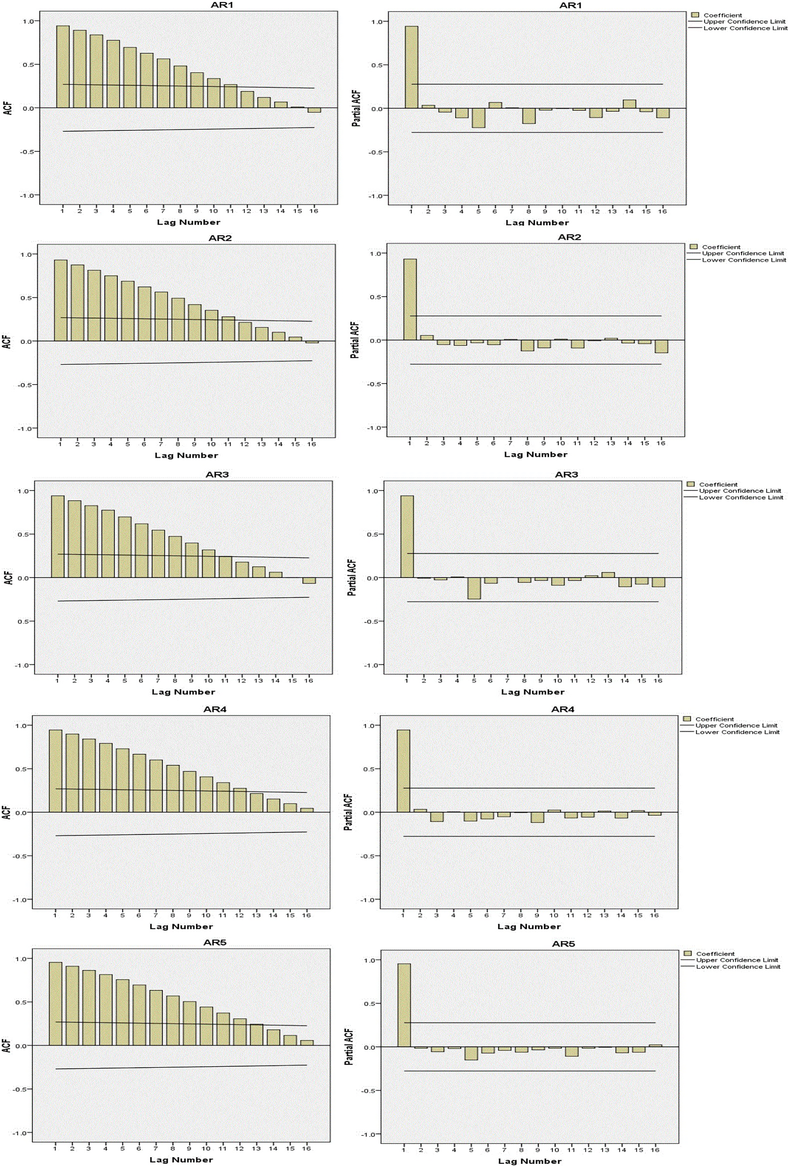
Sample ACF (left panels) and sample PACF (right panels). ACF: autocorrelation function; PACF: partial autocorrelation function.

Figure 4.

ACFs (left panels) and PACFs (right panels) of the differenced data series. ACF: autocorrelation function; PACF: partial autocorrelation function.

Table 2.

Estimated parameter values for seasonal ARIMA models.

Series	Model	AR	MA	SAR	SMA
AR1	ARIMA(0,1,3)(0,1,1) _L		MA(l) = 0.34 lMA(2) = −0.l0 lMA(3) = −0.295		SMA(l) = 0.447
AR1	ARIMA(0,1,1)(0,1,1) _L		MA(l) = 0.3l7		SMA(l) = 0.290
AR2	ARIMA(0,1,0)(2,0,0) _L			SAR(1) = 0.038SAR(2) = 0.348
AR2	ARIMA(0,1,0)(0,0,2) _L				SMA(l) = −0.005SMA(2) = −0.368
AR3	ARIMA(0,1,0)(1,0,0) _L			SAR(l) = 0.562
AR3	ARIMA(0,1,0)(0,1,0) _L			SAR(l) = 0.562
AR4	ARIMA(1,1,0)(0,1,0) _L	AR(l) = −0.4l9
AR4	ARIMA(0,1,1)(0,1,0) _L		MA(l) = 0.404
AR5	ARIMA(0,1,0)(0,1,1) _L				SMA(l) = 0.554
AR5	ARIMA(0,1,0)(0,1,0) _L				SMA(l) = 0.554

ARIMA: autoregressive integrated moving average; AR: autoregressive; MA: moving average; SAR: seasonal autoregressive; SMA: seasonal moving average.

Based on the approach provided by Box et al.,⁴⁷ the model parameters, model fit, and error measures were estimated for the five cost series. In order to select proper seasonal ARIMA models, different models with various combinations of regular orders (p and q) and seasonal orders (P and Q) were evaluated. The model parameters of the five cost series are presented in Table 2. Furthermore, the model fit and error measures of the ARIMA models are provided in Table 3. As seen from Table 3, the values of R ² indicate the ARIMA models fit the cost data fairly well.

Table 3.

Model fit statistics and residual statistics.

Series	Model	R ²	RMSE	MAPE	MAE	BIC	Ljung–Box	Shapiro–Wilk
AR1	ARIMA(0,1,3)(0,1,1) _L	0.959	37.234	1.716	25.866	7.644	0.873	0.461
	ARIMA(0,1,1)(0,1,1) _L	0.953	38.665	1.856	27.895	7.556	0.519	0.158
	ES (AHW)	0.976	33.205	1.655	24.52	7.233	0.238	0.203
	ES (MHW)	0.974	34.311	1.581	23.722	7.299	0.805	0.102
AR2	ARIMA(0,1,0)(2,0,0) _L	0.942	63.899	2.221	38.057	8.546	0.877	0.184
	ARIMA(0,1,0)(0,0,2) _L	0.942	63.865	2.256	38.766	8.545	0.898	0.136
	ES (AHW)	0.947	62.506	2.066	35.292	8.498	0.891	0.153
	ES (MHW)	0.943	64.989	2.159	37.134	8.576	0.904	0.133
AR3	ARIMA(0,1,0)(0,1,0) _L	0.944	54.277	1.913	35.836	8.07	0.855	0.153
	ARIMA(0,1,0)(4,1,0) _L	0.95	53.423	1.823	33.945	8.366	0.956	0.122
	ES (AHW)	0.964	52.405	1.953	36.27	8.146	0.13	0.103
	ES (MHW)	0.959	55.473	2.054	38.568	8.26	0.106	0.173
AR4	ARIMA(1,1,0)(0,1,0) _L	0.981	51.468	1.53	37.383	8.046	0.657	0.391
	ARIMA(0,1,1)(0,1,0) _L	0.981	51.889	1.505	36.868	8.062	0.628	0.24
	ES (AHW)	0.989	45.577	1.32	31.825	7.867	0.593	0.127
	ES (MHW)	0.988	47.836	1.385	34.24	7.964	0.333	0.104
AR5	ARIMA(0,1,0)(0,1,1) _L	0.986	40.162	1.325	27.306	7.55	0.489	0.127
	ARIMA(0,1,0)(0,1,0) _L	0.983	43.299	1.52	31.335	7.618	0.141	0.103
	ES (AHW)	0.991	36.083	1.312	27.824	7.4	0.477	0.393
	ES (MHW)	0.989	39.374	1.356	28.715	7.574	0.415	0.647

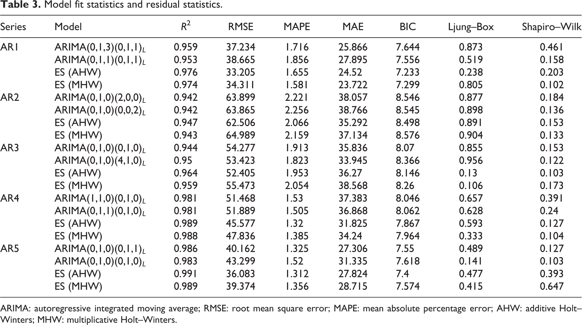
ARIMA: autoregressive integrated moving average; RMSE: root mean square error; MAPE: mean absolute percentage error; AHW: additive Holt–Winters; MHW: multiplicative Holt–Winters.

Model validation

The Ljung–Box Q test was employed to examine the autocorrelation of model residuals. If the p value is greater than the value of 0.05, the null hypothesis that the data are not correlated should be accepted.²⁰ To examine the normality of the residuals, the analysis applied the Shapiro–Wilk test. If the p value of the test is greater than the value of 0.05, it indicates that there is no evidence to reject the null hypothesis that the data follow a normal distribution.⁵³ As seen from Table 3, the residuals of all the models pass the tests, indicating the proposed models are adequate.

Comparisons of the models in the out-of-sample period

Although a model can fit the data fairly well, it does not indicate that the model can produce better forecasts.⁵⁴ The forecasting accuracy of a model is affected by many factors, such as the number of observations in the time series, the number of forecast time origins examined, and the number of forecast lead times regarded.⁵⁵ The forecasting performance of the univariate methods was evaluated by MAPE statistics. The AR1 results presented in Table 4 suggest that the exponential smoothing models generate better results in comparison to seasonal ARIMA models. In particular, the additive Holt–Winters model produces better forecasts based on MAPE measurement. When analyzing the AR2 results, the additive Holt–Winters model outperforms other models based on MAPE measurement. The results regarding AR3, the ARIMA model has the best forecasting performance among the proposed four models. For AR4 suggest that ARIMA(0,1,1)(0,1,0)₄ is the best forecasting model. For AR5, ARIMA(0,1,0)(0,1,1)₄ produced the best forecasts among the proposed models. Therefore, these results suggest that the ARIMA approach is better than the exponential smoothing method for building cost of the town house, apartments, and retirement village in New Zealand. The results show that seasonal ARIMA models perform better for predicting building cost for town house, apartments, and retirement village in New Zealand, while exponential smooth models are superior in cost forecasting for both the one-story house and the two-story house in New Zealand. This outcome may be due to the relative stability of the cost series for the one-story house and the two-story house.

Table 4.

Forecast values for building cost of one-story house in New Zealand.

Series	Model	MAPE
AR1	ARIMA(0,1,3)(0,1,1) _L	1.813
	ARIMA(0,1,1)(0,1,1) _L	1.651
	ES (AHW)	1.260
	ES (MHW)	1.556
AR2	ARIMA(0,1,0)(2,0,0) _L	0.922
	ARIMA(0,1,0)(0,0,2) _L	0.794
	ES (AHW)	0.395
	ES (MHW)	0.650
AR3	ARIMA(0,1,0)(0,1,0) _L	1.020
	ARIMA(0,1,0)(4,1,0) _L	2.318
	ES (AHW)	1.211
	ES (MHW)	1.130
AR4	ARIMA(1,1,0)(0,1,0) _L	0.501
	ARIMA(0,1,1)(0,1,0) _L	0.446
	ES (AHW)	0.748
	ES (MHW)	0.809
AR5	ARIMA(0,1,0)(0,1,1) _L	0.853
	ARIMA(0,1,0)(0,1,0) _L	1.213
	ES (AHW)	0.917
	ES (MHW)	0.949

ARIMA: autoregressive integrated moving average; MAPE: mean absolute percentage error; AHW: additive Holt–Winters; MHW: multiplicative Holt–Winters. The bold-faced values indicate the minimal MAPE of the four models for each cost series.

From the above results, it can be seen that both the exponential smoothing method and the ARIMA approach can produce good forecasts for residential building cost in New Zealand. Which method is better, depends on the characteristics of the data. For example, the ARIMA approach can produce better forecasts for building costs of town house, apartment, and retirement village, which indicates that these costs have a random walk characteristic. The MAPE of the proposed models for all the five cost series are presented in Table 4. Bold type is utilized to identify the lowest values of MAPE for the proposed models of each cost series. As the results show, no single forecasting method is better for all data series. This confirms the generally acceptable idea that no individual forecasting approach can describe all the situations.⁵⁶

Results and discussion

During 2001: Q1–2018: Q4, residential building cost has had an increasing trend. Exponential smoothing approach and ARIMA technique are both effective time series forecasting methods as they both can fairly well describe trend movement in the time series, but they have both strengths and weaknesses. For example, the ARIMA approach is more readily expanded to model interventions, outliers, variations, and variance changes in time series; but it is a relatively sophisticated technique. Due to different data patterns and limited sample size, it is unjust to attempt to determine whether one time series forecasting method is better than the other. Therefore, either the exponential smoothing method or the ARIMA approach should be given a chance to demonstrate its maximum potential in any empirical case study.

While exponential smoothing method is based on describing the trend and seasonality in the time series, ARIMA approach is focused on a description of the autocorrelation in the data. There is an idea that ARIMA approach is more advanced than exponential smoothing method since the former has fewer parameters to be estimated. Although ARIMA models are more general, exponential smoothing models can provide framework that is sufficient to capture the dynamics in the data series. ARIMA models are excellent for short-term forecasting. When they are used for long-term forecasting, the models need to be remodeled based on updated data incorporated into the model training process. exponential smoothing method can be very competitive by automatically incorporating updated information into the model, and then producing better forecasts for long-term forecasting. An advantage of ARIMA technique is that only several parameters need to be estimated for generating good forecasting results. However, extreme values in the data set are difficult to be estimated by ARIMA models due to the univariate nature of the model and the lack of a specific ability to simulate unexpected events.

In this study, exponential smoothing method is an effective tool for forecasting future values of building cost for one-story house and two-story house, while seasonal ARIMA models can produce more accurate forecasts for the building cost series of the town house, apartment, and retirement village in New Zealand. In practice, the fluctuations in building costs for the five categories of residential building in New Zealand differ. For example, building cost series for the one-story house and two-story house show a very consistent repetitive pattern, while the current observations of the cost series for town house, apartment, and retirement village in New Zealand would be affected by the previous observations.

Conclusions

In this study, quarterly building costs data (over an 18-year range from 2001: Q1 to 2018: Q4) for five categories of residential building (one-story house, two-story house, town house, apartment, and retirement village building) in New Zealand were analyzed and the major characteristics of these data were explored. It was found that time series data of residential building costs are nonstationary and autocorrelated and do not display a very strong seasonal pattern. Based on the identified characteristics, two time series forecasting techniques, exponential smoothing method and ARIMA approach, were adopted to take into account variations of residential building costs in predicting their future trends. It was concluded that both methods can produce reliable forecasts. The analysis of model residuals explored that the underlying modeling assumptions hold true. For a given data set, it is almost impossible to know in advance which forecasting method will perform better than others. This is supported by a generally accepted principle that no forecasting approach is better for all situations under all circumstances. From this point of view, the empirical findings of this study suggest that exponential smoothing models can be confidently used to forecast building cost for one-story and two-story houses in New Zealand, while seasonal ARIMA models can produce more accurate cost forecasts for town house, apartment, and retirement village building in New Zealand.

The findings of this study can help construction professionals prepare more accurate cost estimates, improve project cost management, and reduce the risk of cost variations in residential building projects. Residential projects of all types can benefit from the proposed models that improve the accuracy of cost estimates. The study also benefits stakeholders and organizations by improving their understanding of cost management. Moreover, the results also play an important role in guiding policy makers to formulate strategic planning by providing an effective monitoring indicator of construction industry. Additionally, the forecasting model provides an initial foundation for cost index estimates in New Zealand, which may provide a basis for researchers to forecast other cost indices in New Zealand.

It is important to emphasize that residential building costs in New Zealand are difficult to forecast due to many factors which impose pressures on them. Future work may consist of an analysis of the predictors affecting building cost specifically in New Zealand, the application of these forecasting techniques to other building cost such as commercial buildings and industrial buildings, and an analysis of the evolution of building cost by economic sectors. To investigate whether combined forecasting methods and multivariate methods can improve accuracy of cost forecasting. Although this study used the QV’s residential building cost index, the proposed methods can be used for similar data sets in other cities as well as globally. Moreover, although the model can provide accurate cost forecasts, specific features of a construction project should be thoroughly examined in order to generate accurate cost estimates.

Supplemental Material

Supplemental Material, Forecasting-revision - Forecasting residential building costs in New Zealand using a univariate approach

Supplemental Material, Forecasting-revision for Forecasting residential building costs in New Zealand using a univariate approach by Linlin Zhao, Jasper Mbachu and Huirong Zhang in International Journal of Engineering Business Management

Footnotes

Acknowledgments

The authors would like to thank the China Scholarship Council (CSC) for its support through the research project and also the Massey University. The authors also would like to thank the Reserve Bank of New Zealand and the Ministry of Business, Innovation, and Employment for providing data to conduct this research. In addition, the authors would like to thank all practitioners who contributed to this project.

Author contributions

Conceptualization: LZ and JM; methodology: LZ and HZ; software: LZ; validation: LZ; writing—original draft preparation: LZ and HZ; writing—review and editing: JM; supervision: JM; project administration: JM; funding acquisition: LZ.

Data availability

The research data will be provided as request.

Declaration of conflicting interests

The author(s) declared no potential conflicts of interest with respect to the research, authorship, and/or publication of this article.

Funding

The author(s) disclosed receipt of the following financial support for the research, authorship, and/or publication of this article: This research was funded by China Scholarship Council (grant no. 201206130069) and Massey University (grant no. 09166424), and The APC was funded by the both grants.

ORCID iD

Linlin Zhao

References

Ashuri

Shahandashti

. Is the information available from historical time series data on economic, energy, and construction market variables useful to explain variations in ENR construction cost index? In: Construction Research Congress, West Lafayette, Indiana, United States, 21–23 May 2012.

Hwang

. Time series models for forecasting construction costs using time series indexes. J Constr Eng Manage 2011; 137: 656–662.

Ashuri

. Time series analysis of ENR construction cost index. ASCE J Constr Eng Manage 2010; 136(11): 1227–1237.

Moon

. Stochastic forecast of construction cost index using a cointegrated vector autoregression model. J Manage Eng 2013; 29: 10–18.

Touran

Lopez

. Modeling cost escalation in large infrastructure projects. J Constr Eng Manage 2006; 132(1): 853–860.

Ervin

. How to protect profit as material prices rise. Bus J 2007.

Gallagher

. Material price escalation: managing the risks. Construction eNewsletter 2008.

Shahandashti

Ashuri

. Forecasting engineering news-record construction cost index using multivariate time series models. J Constr Eng Manage 2013; 139: 1237–1243.

PwC. Valuing the role of construction in the New Zealand economy. Auckland: PwC, 2016.

10.

MBIE. Briefing for the incoming Minister for Building and Construction. Wellington: Ministry of Business, Innovation & Employment, 2017.

11.

Willis

Rankin

. The construction industry macro maturity model (CIM3): theoretical underpinnings. Int J Prod Perf Manage 2012; 61(4): 382–402.

12.

Harrison

. Can measurement error explain the weakness of productivity growth in the Canadian construction industry? Int Prod Monitor 2007; 14: 53–70.

13.

Rojas

Aramvareekul

. Is construction labour productivity really declining? J Constr Eng Manage 2003; 129: 41–46.

14.

Sui

. The conceptual relationship between construction quality and economic development. Int J Qual Reliab Manage 1993; 10(2): 18–30.

15.

Naderpajouh

Boppana

Hastak

. Need for indices to assess health of the construction industry. In: Construction Research Congress, West Lafayette, Indiana, United States, 21–23 May 2012.

16.

Holt

. Forecasting trends and seasonals by exponentially weighted moving averages. ONR Memorandum 1957; 52(52): 5–10.

17.

Brown

. Statistical forecasting for inventory control. New York: McGraw-Hill, 1959.

18.

Winters

. Forecasting sales by exponentially weighted moving average. Manage Sci 1960; 6: 324–342.

19.

Hyndman

Koehler

Ord

, et al. Forecasting with exponential smoothing: the state space approaches. Berlin: Springer-Verlag, 2008.

20.

Box

GEP

Jenkins

Reinsel

. Time series analysis: forecasting and control. 5th ed. Oakland: Holden-Day, 2011.

21.

Ashuri

. Forecasting ENR construction cost index: a time series analysis approach. In: Construction Research Congress, Banff, Alberta, Canada, 8–10 May 2010.

22.

Gujarati

. Basic econometrics. Rio de Janeiro: Elsevier, 2006.

23.

Taylor

Bowen

. Building price-level forecasting: an examination of techniques and applications. Constr Manage Econ 1987; 5(1): 21–44.

24.

Trost

Oberlender

. Predicting accuracy of early cost estimates using factor analysis and multivariate regression. J Constr Eng Manage 2003; 129(2): 198204.

25.

Cheung

Skitmore

, et al. An integrated regression analysis and time series model for construction tender price index forecasting. Constr Manage Econ 2004; 22(5): 483–493.

26.

Hwang

. Dynamic regression models for prediction of construction costs. J Constr Eng Manage 2009; 135: 360–367.

27.

Hwang

Liu

. Contemporaneous time series and forecasting methodologies for predicting short-term productivity. J Constr Eng Manage 2010; 136(9): 1047–1055.

28.

AbouRizk

. Automated Box–Jenkins forecasting modelling. Automat Constr 2009; 18(5): 547–558.

29.

Fellows

. Escalation management: forecasting the effects of inflation on building projects. Constr Manage Econ 1991; 9(2): 187–204.

30.

Wong

JMW

Chan

Chiang

. Time series forecasts of construction labor market in Hong Kong: the Box-Jenkins approach. Constr Manage Econ 2005; 23(9): 979–991.

31.

Williams

. Predicting changes in construction cost indexes using neural networks. J Constr Eng Manage 1994; 120(2): 306–320.

32.

Kim

Kang

. Comparison of construction cost estimating models based on regression analysis, neural networks, and case-based reasoning. Build Environ 2004; 39(10): 1235–1242.

33.

Cheng

Hoang

. Hybrid intelligence approach based on LS-SVM and differential evolution for construction cost index estimation: a Taiwan case study. Autom Constr 2013; 35: 306–313.

34.

Cao

Cheng

. Hybrid computational model for forecasting Taiwan construction cost index. J Constr Eng Manage 2015; 141: 1–11.

35.

Pierce

Huynh

Guimaraes

. Cost indexing and unit price adjustments for construction materials. Report no. FHWA-SC-12-06, GT-12-01, 30 October 2012. Columbia, SC United State: University of South Carolina. https://rosap.ntl.bts.gov/view/dot/25179.

36.

Smith

Miller

Christofferson

, et al. Best practices for dealing with price volatility in Utah’s residential construction market. Int J Constr Educ Res 2011; 7(3): 210–225.

37.

Weidman

Miller

Christoffersen

, et al. Best practices for dealing with price volatility in commercial construction. Int J Constr Educ Res 2011; 7(4): 276–293.

38.

Hwang

Park

Lee

, et al. Automated time-series cost forecasting system for construction materials. J Constr Eng Manage 2012; 138(11): 1259–1269.

39.

Nam

Han

Kim

. Time series analysis of construction cost index using wavelet transformation and a neutral network. In: 24th International Symposium on Automation & Robotics in Construction, IIT Madras, 19–21 September 2007. Madras, India: Indian Institute of Technology Madras.

40.

QV. Construction cost index. Wellington, New Zealand: QV, 2018.

41.

Arlot

Alain

. A survey of cross-validation procedures for model selection. Statis Survey 2010; 4: 40–79.

42.

Chatfield

. Time series forecasting. London: Chapman & Hall/CRC, 2001.

43.

Bowerman

O’Connell

Koehler

. Forecasting, time series, and regression. Boston: Thomson Learning Inc., 2005.

44.

Hyndman

Koehler

Snyder

, et al. A state space framework for automatic forecasting using exponential smoothing methods. Int J Forec 2002; 18(3): 439–454.

45.

Gardner

Jr ES

. Exponential smoothing: the state of the art. Int J Forec 2006; 22(4): 637–666.

46.

Maia

ALS

de Carvalho

FAT

. Holt’s exponential smoothing and neural network models for forecasting interval-valued time series. Int J Forec 2011; 27(3): 740–759.

47.

Box

GEP

Jenkins

Reinsel

. Time series analysis: forecasting and control. 3rd ed. New Jersey: Prentice Hall, 1994.

48.

Taneja

Ahmad

, et al. Time series analysis of aerosol optical depth over New Delhi using Box–Jenkins ARIMA modeling approach. Atmos Pollut Res 2016; 7: 585–596.

49.

Ljung

Box

. On a measure of a lack of fit in time series models. Biometrika 1978; 65: 297–303.

50.

Krol

. Evaluating state revenue forecasting under a flexible loss function. Int J Forec 2013; 29(2): 282–289.

51.

Kankal

Uzlu

. Neural network approach with teaching–learning-based optimization for modelling and forecasting long-term electric energy demand in Turkey. Neural Comput Appl 2016; 28: 737–747.

52.

Musttaffa

Yusof

Kamaruddin

. Enhanced artificial bee colony for training least squares support vector machines in commodity price forecasting. J Comput Sci 2014; 5(2): 196–205.

53.

Hanusz

Tarasinska

Zielinski

. Shapiro–Wilk test with known mean. REVSTAT- Stat J 2016; 14(1): 89–100.

54.

Makridakis

Wheelwright

Hyndman

. Forecasting: methods and applications. 3rd ed. New York: John Wiley & Sons, 1998.

55.

Pack

. In defense of ARIMA modelling. Int J Forec 1990; 6: 211–218.

56.

Chatfield

. What is the best method of forecasting? J Appl Stat 1988; 15(1): 19–38.

Supplementary Material

Please find the following supplemental material available below.

For Open Access articles published under a Creative Commons License, all supplemental material carries the same license as the article it is associated with.

For non-Open Access articles published, all supplemental material carries a non-exclusive license, and permission requests for re-use of supplemental material or any part of supplemental material shall be sent directly to the copyright owner as specified in the copyright notice associated with the article.

0.00 MB

2.06 MB