Sage Journals: Discover world-class research

Abstract

The literature has several models that jointly determine the economic production quantity (EPQ) and the rate of production. Very few models define production rate explicitly. In this article, the cutting speed controls the production rate and the proportion nonconforming. Thus, we propose a model that integrates EPQ, machining economics and quality. Even though the objective function of the model is non-convex, we show for realistic values of some technical parameters that a local minimum of the proposed mathematical model is also global. Examples clearly show the effect of the production economics factors on the optimal machining speed and production quantity.

Keywords

Production planning and controlling manufacturing quality control industrial engineering manufacturing planning and execution

Introduction

The economic production quantity (EPQ) is a well-known concept in operations management. Over the past hundred years, thousands of papers have found the optimal production quantity for different scenarios.¹ EPQ is the batch size that a manufacturer produces to satisfy a certain demand and minimize the production cost. In its basic form, the EPQ seeks to find the best trade-off between holding and setup costs. Finding the optimal trade-off between inventory and the frequency of production/replenishment orders leads to substantial savings in operations costs.²

Many researchers studied different settings and extensions of this classical problem. These include, but are not limited to, integrated models,³ bundling strategies,⁴ variable lead-time,⁵ variable production rate,⁶ and variable holding cost.⁷ Several survey papers can be found on this problem and its variations, as examples: Glock,⁸ Ramasesh,⁹ Drexl and Kimms,¹⁰ and Zoller and Robrade.¹¹

Most EPQ models assume a constant production rate. In practice, the production rate of a manufacturing facility can be controlled either by varying the manufacturing equipment rate or by inserting idle times between jobs.¹² Production rate is an essential control parameter in any industry, because it affects equipment availability, productivity, and quality. In machining economics, cutting speed is a key decision variable, and it has a direct link to the production rate.¹³

To the best of our knowledge, in comparison to fixed production rate models, variable production rates are not well-studied in the literature.^12,14,15 Further, variable production rate models rarely define an explicit mechanism to vary the rate of production, rather a unit production cost function is usually assumed.¹⁶ This article contributes to the literature by considering quality in an economic lot sizing and machining economics model with variable production rates. The authors are unaware of any model in the literature that accounts for quality within the context of integrated machining economics and economic lot sizing. Furthermore, the behavior of the model is characterized with respect to the model parameters and the global optimal solutions are obtained. To the best of the authors’ knowledge, this point has not been addressed in the literature.

The rest of this article is organized as follows: the second section presents the relevant literature review, the mathematical model is provided in the third section, the fourth section presents some illustrative examples, and the fifth section concludes the article.

Literature review

Variable production rates in lot sizing models

Contrary to most EPQ models that assume fixed production rate, Gallego⁶ distinguished two approaches to production-rate control. The first is flexible where the production rate is allowed to change at any time, while the second is rigid where the production rate is set once at the beginning of a production run.

Some of the models that consider production rate as a decision variable assume that the unit production cost is a convex function of the production rate. Khouja¹⁷ included the production rate as a decision variable in determining the single-product EPQ. Unit production cost was assumed to be a convex function of the production rate. The author showed that the more volume-flexible a production system is, the larger the EPQ and the smaller the optimal production rates are. Eiamkanchanalai and Banerjee¹⁸ considered a single-product economic run length with variable production cost for the two cases: with and without idle capacity cost. The authors discussed the effect of idle capacity cost on the economic run length and economic production rate.

Glock¹² addressed the case of batch sizing with controllable production rates for equal- and unequal-sized batch shipments. The author showed that deviating from the design production rate of a production system can be advantageous for holding and total costs. Glock¹⁴ extended his previous model¹² to a serial production line and showed that varying the production rate of a system depends on factors related to the number of batch shipments, adjacent stage rates, and inventory holding cost of the buffers before and after a given production stage. The author also underlined the advantage of reducing inventory cost. AlDurgam et al.¹⁵ extended the works of Glock^12,14 by considering variable production rates in a two-echelon supply chain with stochastic demand and demonstrated that considering variable production rates can benefit the supply chain members.

In production processes that involve metal cutting operations, the production rate can be directly controlled by varying the cutting speed. This, however, involves some cost trade-offs. Building on the work of Taylor,¹⁹ wherein he developed the famous equation that shows the relationship between the cutting speed and the expected tool life, different models have been formulated to determine the optimal cutting speed for machining operations. These models determine the cutting speed to minimize production time or cutting tool cost per produced product. The effect of batch size on the optimal cutting speed was first addressed by Wysk et al.²⁰ He considered lot-size information in the determination of optimal machining speed. On the other hand, Koulamas²¹ developed a model for the joint determination of optimal cutting speed and production lot size to minimize the manufacturing lead-time in multi-stage, multi-product machining systems. Koulamas²² provided a solution methodology that jointly determined the optimal cutting speed and the EPQ under a finite demand rate. The solution method suggested in Koulamas²² guarantees the convergence to local optimal solutions.

The impact of production rate on quality

The majority of EPQ models do not consider production rate²³ and those models that consider production rate ignore its impact on quality. The work of Hui et al.²⁴ is one of few research papers that do not ignore the cost of quality. In that paper, the quality cost depended on the deviation from the targeted roughness and dimensions. The quality cost was incorporated explicitly in the total machining cost function, rather than being a constraint. The model, however, did not target the EPQ.

Owen and Blumenfeld²⁵ considered the impact of cutting speed on the scrap percentage, which was regarded as the quality cost in their model. A trade-off policy was developed to determine the joint optimal production rate and scrap percentage. Al-Fawzan and Al-Ahmari²⁶ explicitly incorporated cutting speed in a model that determines the optimal process target value for a single machine.

Salameh and Jaber²⁷ developed an EOQ model which assumed that lots are received in batches where the fraction of the nonconforming products follows a known probability distribution and the produced units are subject to 100% inspection. Papachristos and Konstantaras²⁸ examined the model of Salameh and Jaber²⁷ for the non-shortage condition and were able to show that it might not prevent shortage. Wee et al.²⁹ extended the model of Salameh and Jaber²⁷ by allowing backordering, such that shortages are satisfied at the beginning of the cycle before quality screening. Recently, Öztürk et al.³⁰ proposed an EOQ model for lots with shortage and rework option. To justify the rework option, the authors compared their model with the case where rework is not available.

Sana³¹ considered an EPQ model where the fraction of nonconforming products depends on the production rate and production run time. Yassine et al.³² developed an EPQ model which assumed that the fraction of nonconforming products follows a probability distribution function and that the nonconforming products are salvaged. The model further allowed for disaggregating shipments of imperfect quality over single and multiple production runs. Further literature on EPQ models with imperfect quality is provided by Khan et al.³³

Multi-product models

In flexible and make-to-order manufacturing systems, it is not optimal to determine the EPQ for each product separately; this is due to resource sharing such as equipment, space, labor, and budget. Multi-product EPQ models are widely addressed in the literature and under different settings. For example, Guchhait et al.³⁴ examined a model with breakable products with stock-dependent demand and breakability rates. The model had an investment constraint. Due to nonlinearity and complexity of the model, they solved it using the genetic algorithm. The model in Zhou³⁵ replaced the investement constraint by an order size one, where a manufacturer imposes a minimum order size constraint. The author developed a lower bound to the optimal policy and suggested heuristic solution methods to compute the optimal order quantities.

Wu et al.³⁶ presented the problem of scheduling, encountered in the production of multi-product problem. The authors developed a hybrid-nested partitions algorithm for the problem. Chiu et al.³⁷ provided a closed form solution to the problem of determining the EPQ and the optimal rotation cycle of multiple product on a single machine with random defect rate.

Recent works on multi-product economic lot sizing include Taleizadeh et al.³⁸ who developed an EPQ model with process interruption, scrapped, rework, and backorders. Chiu et al.³⁹ developed a multi-product economic manufacturing quantity model involving rework and overtime production. The authors proved convexity of the objective function of their model. Kundu et al.⁴⁰ developed a multi-product production inventory model for seasonal products over a finite planning horizon; the developed model considers rework of items with imperfect quality and variable production cost.

Synthesis of the three research streams

The literature review indicates that variable production rates are not well-studied in the literature.^12,14,15 Further, variable production rate models rarely define an explicit mechanism to vary the rate of production, rather a unit production cost function is usually assumed.¹⁶

In this article, we propose a model that jointly determines the economic batch size and cutting speed, taking production quality into consideration. To the best of our knowledge, this model has not been discussed in the literature. The quality measure used in this article is the proportion of nonconforming units. Previous work ignores this quantity, hence the optimal solution will select the cutting speed and batch size that will minimize cost, but it may result in a high proportion of defective items. This means that further production is needed to satisfy the demand. Obviously, this contradicts the concept lean production. The proposed model considers the following costs: holding cost, setup cost, cutting tool cost, quality cost, and opportunity cost. This article extends the work of Koulamas²² by considering quality using the results of Owen and Blumenfeld.²⁵ Furthermore, we address the cases of single and multi-products and show that the global optimal solution can be obtained using an efficient solution methodology. Lastly, we characterize the behavior of the proposed model with respect to the model parameters theoretically and numerically.

Model development

The EPQ problem assumes that there is an annual demand for a product and the objective is to find the production batch size that results in minimizing the total inventory/holding cost and production setup cost associated with each batch. In this article, we consider a product that is produced through a machining operation. The machine has different settings for the cutting speed. Obviously, the time to finish the operation will depend on the selected speed and this, in turn, will determine the production rate. From a machining perspective, it is known that the cutting speed affects both tool life and the quality of produced products. In general, higher cutting speeds result in shorter tool life but result in better quality surface finish. The problem we address here is determining the cutting speed that will result in minimizing the costs associated with tool life and product quality in addition to the EPQ costs, namely holding cost and setup cost. We propose a mathematical model to address the above scenario assuming the following:

Deterministic demand.^22,41

Batch production.^15,22

Quality cost is represented by the cost of fraction nonconforming.^42,43

Nonconforming products are sold in a secondary market at a reduced price.^42,43

Cutting speed affects cutting time and hence the rate of production.²²

In practice, cutting speed is changed stepwise. However, since step size can be very small, we assume it is continuous in our model.²²

Cutting speed is set once before production starts and stays fixed for the rest of time.^15,22

The time to replace a cutting tool is negligible.

We use machine opportunity cost that is incurred when the machine is in operation. Note that the machine may have idle times. If the production rate is sufficiently high, the generated products will satisfy future demand and the machine will be idle until the extra production is consumed.²²

We assume that the demand is satisfied once the production batch/cycle is completed. In the traditional EPQ models, demand is satisfied as products are produced.⁴¹

The nomenclature used in the mathematical model is provided as follows:

	Parameters
A	Setup cost ($/setup)
c	Constant used in Taylor’s tool life equation
C₀	Opportunity cost associated with the machine run time ($/min)
C_t	Tool cost ($/tool)
D	Annual demand (products/year)
h	Holding cost ($/product/year)
k	Machining constant relating cutting time to cutting speed
k′	Fraction nonconforming multiplier
MPY	Minutes per year, a conversion factor from a year of 200 working days to minutes; used to achieve unit consistency between t_m and T and r and D
n	An exponent used in Taylor’s tool life equation
r_max	Maximum production rate
s₁	Selling price of conforming products ($/product)
s₂	Selling price of nonconforming products ($/product)
v_max	Maximum cutting speed
w	Raw material cost ($/product)
α	Fraction nonconforming exponent
	Auxiliary variables
p	Fraction of nonconforming products in a batch
r	Production rate (products/min)
T	Cycle time (years)
T_p	Production time (years)
t_m	Cutting time per product (min) = 1/r = k/v
τ	Tool life (e.g. 60–120 min for high-speed steel)
	Decision variables
v	Cutting speed (foot/min)
y	Number of units produced per cycle, batch size

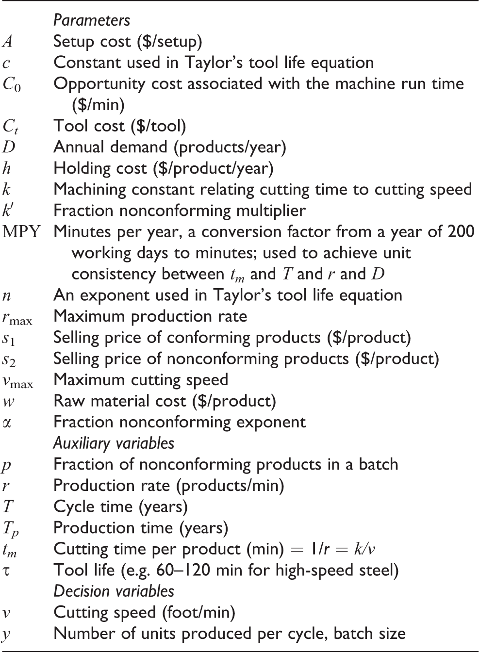
In this article, we consider the EPQ for both single- and multi-products cases. The “Single-product model” section discusses the case of producing one product while the “Multi-product model” section under “Model development” is about production of several products.

Single-product model

In this section, we construct a mathematical model that accounts for all costs associated with production, holding inventory and machine setup. The model will be used to determine the EPQ and the optimal production rate for a single product.

We consider manufacturing operations where the cutting speed, v, does not change at different production stages. These include facing using a milling machine or a lathe. It also includes drilling. In this case, the cutting time, t_m , depends on the length of the part or the depth of the hole. Hence t_m = k/v, where k is a constant related to the length of the surface being faced and conversion of units of measurements. We assume that the time between completion of cutting of a product and the start of cutting of the next product is negligible. This is valid if the products are laid next to each other on the machine bed or special jigs and fixtures are used. In this case, the production rate r is inversely proportional to the cutting speed, r =v/k.

Owen and Blumenfeld²⁵ suggested a relation to express the fraction nonconforming, p, as a function of the production rate, where p = k′(r/r _max) ^α . The parameters α and k′ are process dependent and α ≥ 1. This relation shows that the proportional nonconforming is an increasing function of the production rate.

Cutting speed affects tool life. We estimate tool life using the well-known Taylor formula vτⁿ = c, where n and c are parameters that depend on cutting tool material and cutting conditions.

Figure 1 presents inventory buildup during a cycle of length T at two different production rates: r ₁ and r ₂, where r ₂ > r ₁. The same batch size, y, is produced at both rates. Hence, p ₂ > p ₁ and T_p ₁ > T_p ₂. The problem is to select the optimal values of y and r that minimize the total production cost per unit time. The total production cost is composed of several elements which we will describe next. In our model, r is considered as a function of the cutting speed, hence, an optimal value of v leads to the optimal value of r.

Figure 1.

Inventory buildup at different production speeds.

Assuming that a setup cost is incurred each time a batch is produced, the average annual setup cost is equal to A(D/y). The average annual on hand inventory is 0.5yT_p /T, where T_p is the production time during a typical cycle of length T. Since T_p = y/(r·MPY) and T = y/D, the average annual inventory is given by yD/(2r·MPY).

We estimate the per-product tool cost as C_tt_m /τ, as recommended by Al-Fawzan and Al-Ahmari.²⁶

Recalling that D products are produced per year, the annual tool cost is equal to D·C_t (k/v)/(c/v)^1/n.

At each production cycle, py nonconforming units are produced. Hence, the annual number of nonconforming products is pD. Using this relationship, the number of nonconforming products per year is k′(r/r _max) ^αD. Finally, the opportunity cost of machine time per product is C ₀ t_m which is C ₀ Dk/v per year. The total cost per year is the sum of the setup cost, holding cost, materials cost, quality cost, tool cost, and opportunity cost.

In case of a single-product case we solve the following mathematical program:

Minimize

F (y, r, v) = A D / y + h y D / (2 r \cdot MPY) + w D + k' {(r / r_{max})}^{α} D (s_{1} - s_{2}) + D C_{t} \frac{k}{v} / {(\frac{c}{v})}^{\frac{1}{n}} + D C_{0} \frac{k}{v}

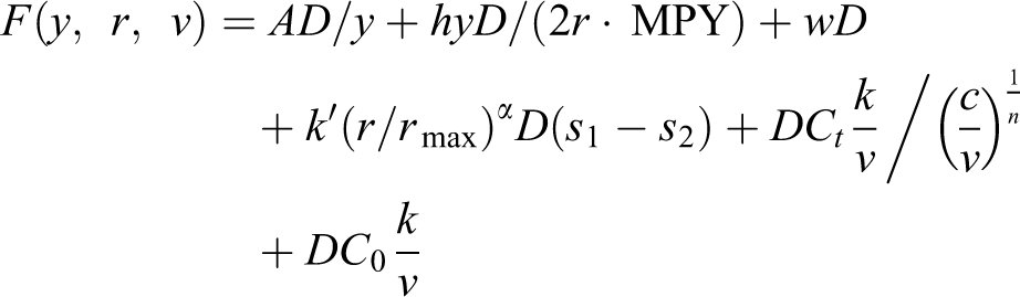
subject to:

r \times MPY \geq D

r \leq r_{max}

y \geq 0

MPY is used to maintain the unit consistency between the left and right sides of constraint (1). Constraint (2) ensures that the production rate does not exceed the machine capability.

Since r = 1/t_m = v/k, the above mathematical program can be expressed as follows:

Minimize

Z (y, v) = \frac{A D}{y} + h y D k / (2 v . MPY) + w D + k' {(v / v_{max})}^{α} D (s_{1} - s_{2}) + D C_{t} \frac{k}{v} / {(\frac{c}{v})}^{\frac{1}{n}} + D C_{0} \frac{k}{v}

subject to:

D k / (v \cdot MPY) \leq 1

v \leq v_{max}

y \geq 0

Note that when constraint (4) is binding, that is, satisfied as a strict equality, and if the quality cost is ignored, then the cutting speed becomes known and the model reduces to the classical EPQ model with the optimal batch size equal to $\sqrt{2 A D / h}$ .

Theorem 1

For n ≤ 0.5 and α ≥ 1, a local minimum solution to the above mathematical program is also global.

Proof

Z(y,v) is non-convex, since the second term is quasi-linear. For any v that satisfies constraints (4) and (5), the resulting objective is a convex function of y. Setting dZ/dy to 0, gives a unique solution, y*, where $y^{*} (v) = \sqrt{2 MPY \cdot A \cdot v / (h \cdot k)}$ . Let $H (v) = Z (y^{*} (v), v)$ , then

H (v) = D \sqrt{2 A \cdot h \cdot k / (MPY \cdot v)} + w D + k' {(v / v_{max})}^{α} D (s_{1} - s_{2}) + D \cdot C_{t} \frac{k}{v} {(\frac{v}{c})}^{\frac{1}{n}} + D \cdot C_{0} \frac{k}{v}

Note that a function of the form v^t is convex for $t \leq 0$ and $t \geq 1$ . Each term in $H (v)$ is a function of the form v^t . The third term is convex if $α \geq 1,$ while the fourth term is convex if $n \leq 0.5$ . The sum of convex functions is convex hence $H (v)$ is a convex function of v for $n \leq 0.5$ and $α \geq 1$ . Hence a local minimum of $Z (y, v)$ is also global. This completes the proof.

The minimum of $H (v)$ , where $D k / MPY \leq v \leq v_{max}$ could be found by any line search method.

Remark

Koulamas²² reported that $n \leq 0.5$ covers a wide range of cutting tools, such as high-speed steel and cemented carbide and ceramic. On the other hand, $α = 1$ was suggested by Owen and Blumenfeld.²⁵ In general, the theorem applies for any quality cost function, provided that it is convex (e.g. Taguchi quadratic function). Several models in the literature assume linear or quadratic quality cost functions, but the one proposed by Owen and Blumenfeld²⁵ was used because it directly links fraction nonconforming to the cutting speed.

Multi-product model

In this section, we consider the production of J products on the same machine. Each product has its EPQ and economic cutting speed. The multi-product model is given by:

Minimize

Z (y_{1}, v_{1}, y_{2}, v_{2} \dots y_{J}, v_{J}) = \sum_{i = 1}^{J} D_{i} [A_{i} / y_{i} + h_{i} \cdot y_{i} \cdot k_{i} / (2 v_{i} \cdot MPY) + w_{i} + {k'}_{i} {(v_{i} / v_{max}_{i})}^{α_{i}} (s_{1}_{i} - s_{2}_{i}) + C_{t}_{i} \cdot k_{i} / v_{i} {(\frac{v_{i}}{c_{i}})}^{\frac{1}{n_{i}}} + C_{0} k_{i} / v_{i}]

subject to:

v_{i} \geq k_{i} D_{i} / MPY i \in {1, 2, 3 \dots J}

v_{i} \leq v_{max}_{i} i \in {1, 2, 3 \dots J}

y_{i} \geq 0 i \in {1, 2, 3 \dots J}

\sum_{i = 1}^{J} k_{i} \cdot D_{i} / (v_{i} \cdot MPY) \leq 1

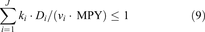
The multi-product model is similar to the single-product model except for constraint (9), which ensures that machine capacity is not exceeded when several products are processed on the same machine. Note that satisfaction of constraint (9) implies satisfactions of the set of constraints given by constraint (6). Hence we drop the set of constraints given by constraint (6). We do not consider scheduling the products on the machine. For further details on the economic batch scheduling problem, refer to Chan et al.⁴⁴

Theorem 2

For $n_{i} \leq 0.5$ and $α_{i} \geq 1$ , $i = 1, \dots, J$ , a local minimum of the above mathematical program is also global.

Proof

The proof is similar to the single-product case. For any given set of cutting speeds, $v_{1}, v_{2} \dots, v_{J}$ that satisfy constraints (6) to (9), the objective function above is a convex function of $y_{1}, y_{2}, \dots y_{J}$ . Setting the partial derivatives $d Z / d y_{i}$ to 0 yields unique solutions $y_{i}^{*} (v_{i}), i = 1, 2, \dots, J$ , where $y_{i}^{*} (v_{i}) = \sqrt{2 MPY \cdot A_{i} \cdot v_{i} / (h_{i} k_{i})}$ . Let $H (v_{1}, v_{2} \dots, v_{J}) = Z (y_{1} (v_{1}), y_{2} (v_{2}), \dots y_{J} (v_{J}), v_{1}, v_{2} \dots, v_{J})$ .

H is a separable function and is convex in $v_{1}, v_{2} \dots, v_{J}$ for $n_{i} \leq 0.5$ and $α_{i} \geq 1$ . Hence, a local minimum of $Z (y_{1}, v_{1}, y_{2}, v_{2} \dots y_{J}, v_{J})$ is also global. This completes the proof.

Numerical illustrations

In this section, we demonstrate the applicability of the proposed models through a number of numerical examples. In the “Single-product model” section, we provide example on the single-product case and study the effect on the solution when some parameters change their values. The “Multi-product model” section under “Model development” is for the case of multi-product.

Single-product examples

This section presents two examples on the single-product problem that differ only in the opportunity cost C ₀. Following each example, we present sensitivity analyses.

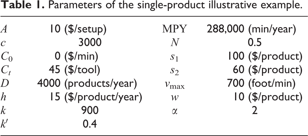
Example 1

Table 1 shows the set of parameters used in this example, where the opportunity cost, C ₀ = 0, implying that the machine run time cost is ignored. The optimal solution is $v^{*} = 19.2$ , $y^{*} = 90.5$ , $p^{*} = 0.0003$ , $Z (y^{*}, v^{*}) = 41, 278$ , $T^{*} = 0.022625$ , and $T_{p}^{*} = 0.014729.$ In this example, 65% of the cycle time is used for production and the machine is idle 35% of the time.

Table 1.

Parameters of the single-product illustrative example.

A	10 ($/setup)	MPY	288,000 (min/year)
c	3000	N	0.5
C₀	0 ($/min)	s₁	100 ($/product)
C_t	45 ($/tool)	s₂	60 ($/product)
D	4000 (products/year)	v_max	700 (foot/min)
h	15 ($/product/year)	w	10 ($/product)
k	900	α	2
k′	0.4

Effect of change in D on the solution

Note that the demand, D, is common to all terms of the objective function, hence its effect will be through constraint (4). D appears in the lower limit on the cutting speed. As the demand increases, the lower limit increases. It is easy to show that if D ≤ 6144, then $v^{*} = 19.2$ . If D > 6144, then $v^{*} (D) = D k / MPY$ which is a linear function of D. Also, the optimal production quantity, $y^{*},$ increases proportional to $\sqrt{D}$ . The fraction nonconforming increases proportional to $D^{α} .$ From Theorem 1, $H (v)$ is convex, then for D > 6144, H is increasing function of D.

Effect of change in A on the solution

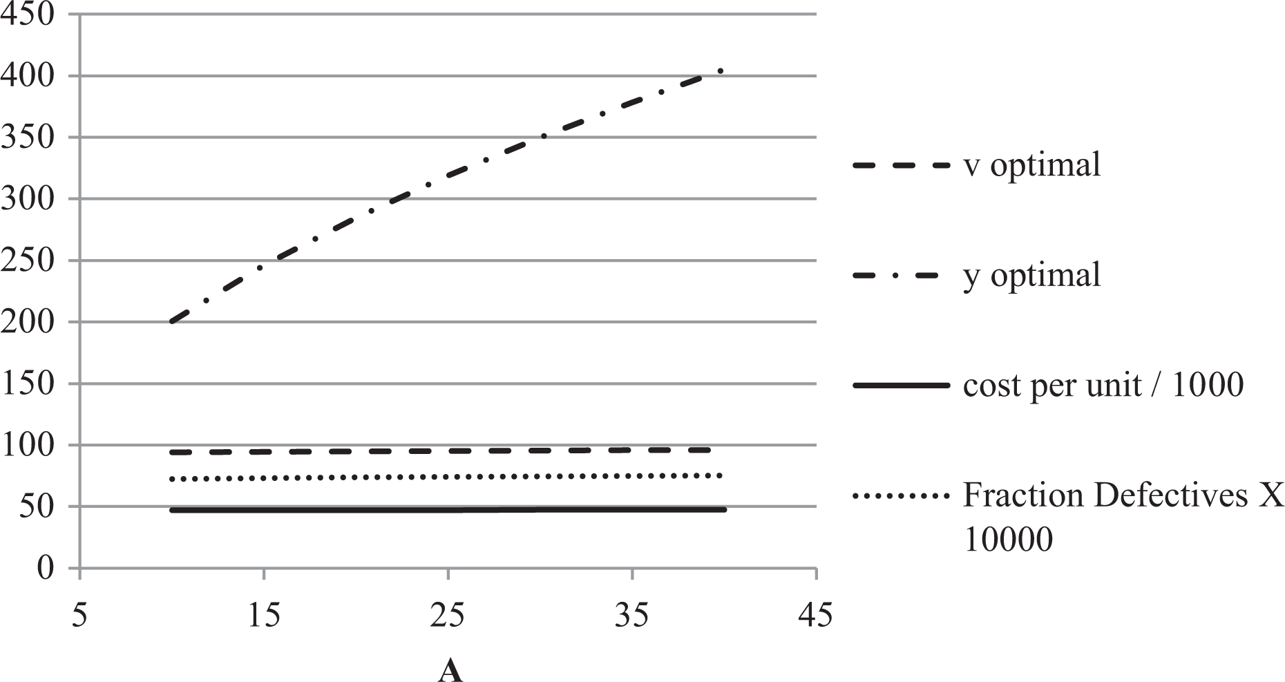
As A increases, the solution will result in less setups hence larger values of $T^{*}$ . Since $T^{*} = y^{*} / D,$ then $y^{*}$ will increase. Note that $y^{*} (v) = \sqrt{2 MPY \cdot A \cdot v / (h \cdot k)}$ , hence $v^{*}$ can be expressed as $β_{1} {(y^{*})}^{2} / A$ where $β_{1}$ is a constant. It is difficult to predict the behavior of $v^{*}$ since the rate of increase in $y^{*}$ is not known to us. The change in $p^{*}$ is similar to that of $v^{*} .$ Figure 2 shows the effect of increasing A on $y^{*}$ and the objective function.

Figure 2.

Effect of the setup cost, A.

The effect of change in h on the solution

Both A and h appear in the numerator of the first term of the objective function, $H (v)$ , hence they have the same effect and $v^{*}$ should increase as discussed earlier. Note that, as in the previous case, $y^{*} (v) = \sqrt{2 MPY \cdot A \cdot v / (h \cdot k)} = β_{2} \sqrt{v / h}$ where $β_{2}$ is a constant, both $v^{*}$ and h are increasing, but since the rate of change of $v^{*}$ is unknown to us, we cannot predict its effect on $y^{*}$ . Figure 3 shows the change in $y^{*}$ and the objective function as h changes.

Figure 3.

Effect of the holding cost, h.

Effect of change in the machining constant, k

k appears in three terms of $H (v)$ as well as constraint (4). Figure 4 shows that as the machining constant, k, increases, the optimal production quantity decreases the cutting speed and the fraction of nonconforming products.

Figure 4.

Effect of the machining constant, k.

Effect of tool change in cost C_t on the solution

C_t appears only in the fourth term of $H (v)$ . An increase in C_t results in a decrease in $v^{*}$ to reduce the tool cost. This in turn will reduce the production level, $y^{*}$ and the proportion nonconforming $p^{*}$ .

Effect of change in n on the solution

Figure 5 shows that as the Taylor exponent increases, the cutting speed decreases, which results in a decrease in both the optimal production quantity and the fraction of nonconforming products.

Figure 5.

Effect of Taylor’s exponent, n.

Effect of change in the opportunity cost C ₀ on the solution

C ₀ appears only in the last term of $H (v)$ . Increasing C ₀ is compensated for by increasing $v^{*}$ to reduce the time the machine is run. This will result in increasing both $y^{*}$ and $p^{*}$ .

Example 2

In this example, we consider the same data of Example 1, except for the opportunity cost, C ₀, which equals $0.1/min. The optimal solution is $v^{*} = 94.27$ , $y^{*} = 200.58$ , $p^{*} = 0.0073$ , $Z (y^{*}, v^{*}) = 47, 075$ , $T^{*} = 0.05014$ , and $T_{p}^{*} = 0.00665.$ Here, the production time is 13.3% of the cycle time. The large drop in machine utilization is a response to the increase in the machine opportunity cost.

When considering the effect of change of A, we find that Figure 6 exhibits the same behavior as that in Figure 2. The increase in the optimal cutting speed results in the increase of y, p, and cost per unit.

Figure 6.

Effect of the setup cost, A, with C₀ = 0.1.

Similarly, if we consider the effect of changing h, we find that Figure 7 exhibits the same behavior as Figure 3. The increase in the optimal cutting speed results in the increase of $y^{*}$ , $p^{*}$ , and the cost per unit.

Figure 7.

Effect of the holding cost, h, with C₀ = 0.1.

Multi-product examples

In this section, we demonstrate the multi-product case by considering three products. In Example 3, the solution satisfies constraint (9) as a strict inequality, while in Example 4, constraint (9) is active or binding.

Example 3

We use the same parameters as in Example 1 except for k, D, h, and s ₁. The following table shows the parameters of each product as well as the optimal cutting speed and production quantity.

Product	k	D	h	s₁	v*	y*
1	900	4000	15	100	94.27	200.58
2	950	6000	10	85	104.5	252.07
3	800	3000	20	140	77.44	166.92

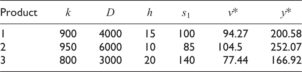
The total cost is 140,502.6. Note that $\sum_{i = 1}^{3} k_{i} \cdot D_{i} / (v_{i} \cdot MPY) = 0.4291 < 1$ , hence constraint (9) is not binding.

Example 4

The data in this example is same as those used in Example 3, except for the demand, where $D_{1} = 40, 000$ , $D_{2} = 60, 000$ , and $D_{3} = 30, 000$ . The optimal solution is $v_{1}^{*} = 401.61$ , $y_{1}^{*} = 413.94$ , $v_{2}^{*} = 468.24$ , $y_{2}^{*} = 532.82$ , $v_{3}^{*} = 313.20$ , $y_{3}^{*} = 335.78$ , total cost = 222,061.2, and $\sum_{i = 1}^{3} k_{i} \cdot D_{i} / (v_{i} \cdot MPY) = 1$ .

Conclusion and managerial insights

This article considers the problem of determining the batch size and cutting speed that result in minimum production cost for single- and multi-product cases. The mathematical model includes, in addition to the standard EPQ costs, the cost of tools and the cost of quality. The function of the total cost is not convex because it includes a quasi-linear term, y/v. Nevertheless, we show that the global minimum cost is obtained. In the above models, and indeed in the literature, it is assumed that tool change times are negligible. If this is not the case, then the attainment of a global solution is questionable. We show through some examples that machining parameters have an impact on the EPQ decision and the optimal cutting speed, justifying the integrated model approach.

Sensitivity analyses show that changing the setup cost, A, in a wide range, will affect very slightly the optimal cost per unit, the fractional nonconforming, p, and the cutting speed, v. This implies that the solution is robust for errors in estimating the setup cost. The only quantity that will increase significantly is the batch size y. This is not an issue for the decision maker if there is no shortage of storage space. If space is an issue, estimating A precisely becomes important. Then steps should be taken to accommodate the large batch size which include acquiring storage space or arranging for speedy delivery to customers.

Large changes in the holding cost, h, does not change the optimal cost per unit, changes the fractional nonconforming, p, very slightly, and increases the cutting speed slightly. Increasing h results in decreasing the batch size which does not cause any problem to the decision maker. Hence, imprecise estimation of h has no negative effect on the solution.

Estimation of the machining constant, k, requires experimentation and time. Luckily, it does not affect the optimal cost per unit, the fractional nonconforming, p, and the cutting velocity, v. It results in a decrease in the batch size, y, which does not raise any issue to the decision maker. Hence, a rough estimate of k is acceptable.

Estimation of the parameter, n, of Taylor’s tool life formula requires experimentation and time. Changes in n do not affect the cost per unit. However, as n increases, p, v, and y decrease. Hence, an error in estimating n on the high side results in smaller fractional nonconforming, p, and batch size, y.

In conclusion, this research work presented a relationship between quality, expressed as fraction nonconforming, and cutting speed. The literature lacks models that take quality into consideration. However, in practice, quality is affected by raw material and tool types; thus, this is an area which warrants further investigation.

Footnotes

Declaration of conflicting interests

The author(s) declared no potential conflicts of interest with respect to the research, authorship, and/or publication of this article.

Funding

The author(s) disclosed receipt of the following financial support for the research, authorship and/or publication of this article: This research is supported by the Deanship of Scientific Research, King Fahd University of Petroleum & Minerals, Dhahran, Saudi Arabia, under project no. JF101011.

ORCID iD

Mohammad M AlDurgam

References

Taleizadeh

Kalantari

Cárdenas-Barrón

. Determining optimal price, replenishment lot size and number of shipments for an EPQ model with rework and multiple shipments. J Ind Manag Optim 2015; 11(4): 1059–1071.

Baciarello

D’Avino

Onori

, et al. Lot sizing heuristics performance. Int J Eng Bus Manage 2013; 5: 5.

Ettaye

El Barkany

Jabri

, et al. Optimizing the integrated production and maintenance planning using genetic algorithm. Int J Eng Bus Manage 2018; 10: 1–9.

Yassine

AlSagheer

Azzam

. A bundling strategy for items with different quality based on functions involving the minimum of two random variables. Int J Eng Bus Manage 2018; 10: 1–9.

Ben-Daya

Hariga

. Integrated single vendor single buyer model with stochastic demand and variable lead time. Int J Prod Econ 2004; 92(1): 75–80.

Gallego

. Reduced production rates in the economic lot scheduling problem. Int J Prod Res 1993; 31: 1035–1036.

Alfares

. An EPQ model with variable holding cost. Int J Ind Eng 2012; 19(5): 232–240.

Glock

. The joint economic lot size problem: a review. Int J Prod Econ 2012; 135(2): 671–686.

Ramasesh

. Lot-sizing decisions under limited-time price incentives: a review. Omega 2010; 38(3–4): 118–135.

10.

Drexl

Kimms

. Lot sizing and scheduling—survey and extension. Eur J Oper Res 1997; 99(2): 221–235.

11.

Zoller

Robrade

. Dynamic lot sizing techniques: survey and comparison. J Oper Manag 1988; 7(3–4): 125–148.

12.

Glock

. Batch sizing with controllable production rates. Int J Prod Res 2010; 48(20): 5925–5942.

13.

Kalpakjian

Schmid

. Manufacturing engineering and technology. London: Pearson, 2014.

14.

Glock

. Batch sizing with controllable production rates in multi-stage production systems. Int J Prod Res 2011; 49(20): 6017–6039.

15.

AlDurgam

Adegbola

Glock

. A single-vendor single-manufacturer integrated inventory model with stochastic demand and variable production rate. Int J Prod Econ 2017; 191: 335–350.

16.

AlDurgam

. An integrated inventory and workforce planning Markov decision process model with a variable production rate. Accepted by the 9th IFAC conference MIM 2019, Berlin, Germany, August 2019.

17.

Khouja

. The economic production lot size model under volume flexibility. Comput Oper Res 1995; 22(5): 515–523.

18.

Eiamkanchanalai

Banerjee

. Production lot sizing with variable production rate and explicit idle capacity cost. Int J Prod Econ 1999; 59(1–3): 251–259.

19.

Taylor

. On the art of cutting metals. New York: American Society of Mechanical Engineers, 1907.

20.

Wysk

Davis

Tanchoco

JMA

. Machining parameter optimization with lot size considerations. AIIE Trans 1980; 12(1): 59–63.

21.

Koulamas

. Lot sizing and machining economics: the multi-item, multi-stage cost minimization case. Int J Prod Res 1992; 30(10): 2265–2280.

22.

Koulamas

. Simultaneous determination of the cutting speed and lot size values in machining systems. Eur J Oper Res 1995; 84(2): 356–370.

23.

Khouja

Mehrez

. Economic production lot size model with variable production rate and imperfect quality. J Oper Res Soc 1994; 45(12): 1405–1417.

24.

Hui

Leung

Linn

. Optimal machining conditions with costs of quality and tool maintenance for turning. Int J Prod Res 2001; 39(4): 647–665.

25.

Owen

Blumenfeld

. Effects of operating speed on production quality and throughput. Int J Prod Res 2008; 46(24): 7039–7056.

26.

Al-Fawzan

Al-Ahmari

AMA

. Simultaneous determination of the optimal process mean and cutting speed for a manufacturing process. Prod Plan Control 2004; 15(3): 336–341.

27.

Salameh

Jaber

. Economic production quantity model for items with imperfect quality. Int J Prod Econ 2000; 64(1–3): 59–64.

28.

Papachristos

Konstantaras

. Economic ordering quantity models for items with imperfect quality. Int J Prod Econ 2006; 100(1): 148–154.

29.

Wee

Chen

. Optimal inventory model for items with imperfect quality and shortage backordering. Omega 2007; 35(1): 7–11.

30.

Öztürk

Eroglu

Lee

. An economic order quantity model for lots containing defective items with rework option. Int J Ind Eng 2016; 22(6): 683–704.

31.

Sana

. An economic production lot size model in an imperfect production system. Eur J Oper Res 2010; 201(1): 158–170.

32.

Yassine

Maddah

Salameh

. Disaggregation and consolidation of imperfect quality shipments in an extended EPQ model. Int J Prod Econ 2012; 135(1): 345–352.

33.

Khan

Jaber

Guiffrida

, et al. A review of the extensions of a modified EOQ model for imperfect quality items. Int J Prod Econ 2011; 132(1): 1–12.

34.

Guchhait

Maiti

. Multi-item inventory model of breakable items with stock-dependent demand under stock and time dependent breakability rate. Comput Ind Eng 2010; 59: 911–920.

35.

Zhou

. Inventory management of multi-item systems with order size constraint. Int J Syst Sci 2010; 41(10): 1209–1219.

36.

Shi

Duffie

. An HNP-MP approach for the capacitated multi-item lot sizing problem with setup times. IEEE Trans Autom Sci Eng 2010; 7(3): 500–511.

37.

Chiu

YSP

Huang

, et al. Joint determination of rotation cycle time and number of shipments for a multi-item EPQ model with random defective rate. Econ Model 2013; 35: 112–117.

38.

Taleizadeh

Cárdenas-Barrón

Mohammadi

. A deterministic multi product single machine EPQ model with backordering, scraped products, rework and interruption in manufacturing process. Int J Prod Econ 2014; 150: 9–27.

39.

Chiu

YSP

Chiu

, et al. Determining the optimal cycle length for a multiproduct EMQ problem considering rework and overtime options. J King Saud Univ Eng Sci 2019; in press.

40.

Kundu

Guchhait

Das

, et al. A multi-item EPQ model with variable demand in an imperfect production process. In: Chandra

Giri

Kar

Jana

(eds) Information technology and applied mathematics. Singapore: Springer, 2019, pp. 217–233.

41.

Ben-Daya

Hassini

Hariga

, et al. Consignment and vendor managed inventory in single-vendor multiple buyers supply chains. Int J Prod Res 2013; 51(5): 1347–1365.

42.

Hanna

Marcus Jobe

. Including quality costs in the lot-sizing decision. Int J Qual Reliabil Manage 1996; 13(6): 8–17.

43.

Hariga

Al-Fawzan

. Joint determination of target value and production run for a process with multiple markets. Int J Prod Econ 2005; 96(2): 201–212.

44.

Chan

Chung

Lim

. Recent research trend of economic-lot scheduling problems. J Manuf Technol Manage 2013; 24(3): 465–482.

Economic production quantity model with variable machining rates and product quality

Abstract

Keywords

Introduction

Literature review

Variable production rates in lot sizing models

The impact of production rate on quality

Multi-product models

Synthesis of the three research streams

Model development

Single-product model

Theorem 1

Proof

Remark

Multi-product model

Theorem 2

Proof

Numerical illustrations

Single-product examples

Example 1

Example 2

Multi-product examples

Example 3

Example 4

Conclusion and managerial insights

Footnotes

Declaration of conflicting interests

Funding

ORCID iD

References