A comparative study of artificial neural network (ANN) and adaptive neuro-fuzzy inference system (ANFIS) models in distribution system with nondeterministic inputs

Abstract

Most deterministic optimization models use average values of nondeterministic variables as their inputs. It is, therefore, expected that a model that can accept the distribution of a random variable, while this may involve some more computational complexity, would likely produce better results than the model using the average value. Artificial neural network (ANN) is a standard technique for solving complex stochastic problems. In this research, ANN and adaptive neuro-fuzzy inference system (ANFIS) have been implemented for modeling and optimizing product distribution in a multi-echelon transshipment system. Two inputs parameters, product demand and unit cost of shipment, are considered nondeterministic in this problem. The solutions of ANFIS and ANN were compared to that of the classical transshipment model. The optimal total cost of distribution using the classical model within the period of investigation was 6,332,304.00. In the search for a better solution, an ANN model was trained, tested, and validated. This approach reduced the cost to 4,170,500.00. ANFIS approach reduced the cost to 4,053,661. This implies that 34% of the current operational cost was saved using the ANN model, while 36% was saved using the ANFIS model. This suggests that the result obtained from the ANFIS model also seems marginally better than that of the ANN. Also, the ANFIS model is capable of adjusting the values of input and output variables and parameters to obtain a more robust solution.

Background

Transshipment problem allows the movement of goods from some source points to some destination points, with the possibility of transshipping through some other source or destination points if it would provide cost benefit. This model is a further generalization of the transportation model because it relaxes the assumption that movement can only be made to a destination point from one or more supply point/s without passing through an intermediate point. This model should be capable of producing a better solution than that of typical transportation problem, if such exists, but it is also known to be more difficult to solve.

The transshipment problem itself is deterministic, and being non-deterministic polynomial-time (NP) hard, solving it is a challenge on its own. Making some of the input parameters nondeterministic makes its solution even more arduous. However, the deterministic transshipment model only uses approximate values of the model parameters, and the extension of the problem to that with some nondeterministic variables is expected to produce a better solution, if tractable. This is what has been done in many stochastic models, and the marginal difference is usually referred to as the value of the stochastic solution. ¹

Representing nondeterminism in input parameters is another interesting issue. While traditionally the nondeterministic variables of most models have been represented in stochastic forms, recent advances in artificial intelligence have brought the use of fuzzy models to prominence. Solutions to stochastic models of linear programming problems (LPPs), for instance, use various techniques that exploit the block separability of the variables, while fuzzy representation makes use of fuzzy operations and fuzzy arithmetic theories. A popular approach of fuzzy logic is based on the fuzzy decomposition theorem and utilizes the properties of alpha cuts along various sections of the fuzzy set. Birge and Louveaux ¹ and Klir and Yuan ² are good readings in order to compare the stochastic LPP and fuzzy modeling and solution approaches to problems.

Finding solution to NP hard problems in itself is difficult; hence, finding solutions to transshipment problems with nondeterministic input parameters could be even more challenging. A number of solutions have been proposed in each case. The main difference in their representation is that while a stochastic model uses an indicator function to allocate a variable to the most likely class in its set based on the estimate of the likelihood of its membership of each set, fuzzy logic assumes that the variable is a member of all of the sets, but by different likelihood of membership. It uses a function ranging from zero to unity to represent the membership across its different sets and uses a different type of set operations from those of probability models to find the variables’ joint membership values. Gaines ³ tried to explain the difference between fuzzy logic and stochastic process in relationship with probability logic, where stochastic processes assume statistical independence and fuzzy logic is purely logical inference.

This article presents solutions to a transshipment problem with nondeterministic input variables in order to estimate the value of the nondeterministic solutions. The demand and unit cost of product distribution were considered to be nondeterministic and solved through adaptive models. Artificial neural network (ANN) model was used to solve the model with stochastic demand and cost variables, while adaptive neuro-fuzzy inference system (ANFIS) was used to solve the same problem with both variables considered fuzzy. The solutions obtained in both cases were then compared. The main difference in these model solutions is in the training paradigm. The data in both cases were separated into training and test samples, and the performance of the test samples in both cases was compared to that of the traditional solution approach. While the manufacturing area seems replete with comparison of these different paradigms of solution in diverse contexts, no author seems to be known in logistics functions, and in transshipment of goods in particular, that has compared the quality of solutions obtained from these two paradigms.

This article is further sectioned as follows: the next section is a presentation of the articles comparing the performance of ANN models to those of ANFIS models in various contexts. The third section is a presentation of the ANN and ANFIS models of the transshipment problem with the two nondeterministic input variables (demand and cost). In the fourth section, the ANN and the ANFIS models were trained, and the levels of fitness achieved were presented. The final section discusses the result of the test sample on the two trained models.

Comparative performance of ANN and ANFIS

ANN and ANFIS performances have been compared in many instances, but mostly in mechanical systems. He et al. ⁴ used both ANN and ANFIS to predict the flow of river in a small river basin in a semiarid mountain region, where the actual mathematical relationships were not fully understood, but the results were observable under diverse conditions. In the study, support vector machine (SVM), ANFIS, and ANN methods were compared. The values of coefficient of correlation (R), root mean squared error, Nash–Sutcliffe efficiency coefficient, and mean absolute relative error were used in assessing the strengths of the three modeling paradigms. The outcome suggests that the three techniques were good enough, while SVM outperforms both ANN and ANFIS. Anari et al. ⁵ did a study on infiltration rate using ANN, ANFIS, local linear regression (LLR), and dynamic LLR and observed that ANFIS appeared to have performed better than all other three techniques.

Do and Chen ⁶ used ANN and ANFIS to forecast post-admission evaluation of students using some preadmission parameters as inputs. They claimed that ANFIS produced better results than ANN. Kamali and Binesh ⁷ used ANN and ANFIS to study the diffusion of water through nanotubes using the molecular dynamics data. They also experimented with data set of different sizes and concluded that ANFIS outperformed ANN. Sredanovic and Dica ⁸ used both ANN and ANFIS to predict the strength of minimal quantity lubrication and high-pressure cooling in the turning task. Both were said to have performed well. Azeez et al. ⁹ compared the performance of ANN and ANFIS in the triage of emergency patients using various vital signs of patients as input parameters. Data were collected from a Malaysian University Hospital. They used ANN backpropagation technique for training, testing, and validation of data set. Fuzzy rules were developed with alpha cuts for ANFIS model, and fuzzy subtractive clustering was used to find the fuzzy rules for the ANFIS model. ANN model gave a better result.

Esen ¹⁰ conducted experiment on heat pump system by comparing the performance of ANFIS and ANN in the upright ground structure. The author stated preference for ANFIS over ANN. Vieira ¹¹ modeled the temperature evolution of a kiln using both the feed-forward ANN and ANFIS system and concluded that ANFIS produced results with less error than the ANN model. Kisi and Ay ¹² compared the performance of radial basis ANN with ANFIS in the study of dissolved oxygen in evaluating water quality. It was established that the ANN model outpaced the ANFIS model. Farahmand et al. ¹³ analyzed the temporal distribution of groundwater contaminants in Iran. They found that ANFIS model outperformed the ANN models, having higher efficiency of estimation. Research areas in other fields of comparative study of ANN and ANFIS are available in the literature but it cannot be said emphatically that either technique always performs better than the other. The performance depends on the context.

There have also been cases where the performance of ANN or ANFIS (or both) has been compared to those of other techniques (like meta-heuristics); or other situations where they have been complementarily applied with other techniques. Li and Chen ¹⁴ used both the least square method (LSM) and the ANFIS to train the artificial systems used in modeling traffic flow in Beijing ring roads and connected lines in order to develop and evaluate the intelligent transport systems. The results obtained from the two approaches were validated against real-life data, and they concluded that model trained with ANFIS produced better results than that trained with LSM. Azadeh and Zarrin ¹⁵ used data envelopment analysis, and meta-heuristics trained ANN and ANFIS logics to evaluate the efficiency of staff along three parameters. It was concluded that ANFIS models trained with genetic algorithm (GA) and particle swarm optimization fared best. Barak and Sadegh ¹⁶ used a combination of autoregressive integrated moving average (ARIMA) and ANFIS to model energy demand. The linear time series parameters were modeled with the ARIMA logic, and the nonlinear residual was later captured using the ANFIS logic in building an expanded model. They concluded that this model performed better than some others. Mansouri et al. ¹⁷ compared the performance of M5Tree, ANN, ANFIS, and multivariate adaptive regression splines (MARS) in analyzing the axial compression of fiber-reinforced polymer and found that ANN predicted an accurate result. Mostafa and El-Masry ¹⁸ used gene expression programming (GEP), ANN, and ARIMA to forecast the evolution of oil prices between January 1986 and June 2016. They reported that both ANN and GEP outperformed ARIMA, and that GEP produced the best result of the three using R ² as the measure of performance. Oduro et al. ¹⁹ did a comparative analysis of the prediction of vehicular emission using boosting MARS (BMARS), classification and regression trees (CART), ANN, and a hybrid of CART–BMARS. They reported that the combined system proved superior to the models of ANN and those of each of the techniques when not hybridized.

While the transshipment problem has been solved using a number of heuristics and meta-heuristics, it is hard to come about those solved using artificial intelligence. Most transshipment models presented recently have been done under the theme of cross-docking. Augustina et al. ²⁰ presented a summary of recent works done on transshipment. They classified the literature into three main categories based on strategic intent and planning horizon: operational, tactical, and strategic. They reviewed some 50 papers. At operational level, the two main issues addressed are about scheduling the cross-docking of trucks and dock-door assignment problems. The most common solution approaches are the different variants of modified Johnson, modified linear programming solution techniques, and meta-heuristics. Tactical-level decision focuses mainly on facility layout decisions, and a number of these problems are solved using meta-heuristics. The long-term decision relates to network design: cross-dock area location and sizes and choice of vehicle sizes and routes. Some other recent papers in the area include a multi-objective GA solution for transportation, assignment and transshipment problems, ²¹ and a Just-in-time (JIT) multi-objective truck forecast problem with door assignment using differential evolution in the cross-dock system. ^22,23

Model notations and formulation

The following notations are adopted for the modeling purpose:

I is the set of all source points, indexed by i and including transshipment points (TPs) as necessary

J is the set of all demand points, indexed by j and including TPs as necessary

K denotes set of TPs, indexed by k

P denotes set of product types, indexed by p

X_ijp is the amount of product p transported from production point i to depots

X_ikp is the amount of product p shipped from production point i to TP k

X_kjp is the amount of product p shipped from TP k to depot j

Z_pi is the capacity of source point i, including the TP, to produce or store product p, whichever is smaller

d_pj is the demand for product p at the destination point j, including the TP

c_pij is the unit amount of transporting product p from production point i to depot j

c_pik is the unit amount of transporting product p from production point i to TP k

c_pkj is the unit amount of transporting product p from TP k to depot j

ξ is a time indexed random vector on which the outcome of the demand and cost depends, which helps to partition decisions into periods before and after the evolution of ω, a random event that affects demand and shipment cost

ω is a random event, $\omega \in \Omega$ , that influences demand and cost of product, p

q is the second-stage objective vector of a stochastic programming model, $q\in Q$

x is the first-stage feasible decision vector, $x\in X$

y is the second-stage feasible decision vector, $y\in Y$

E(·) is the expectation operator

M(·) is the membership function operator

A is the first-stage constraint matrix in a two-stage stochastic model with recourse

h is the RHS vector of the second stage (recourse action) of the stochastic program;

W is the Recourse matrix, based on the values from the evolution of ξ

T is called the Technology matrix such that $Wy=h-Tx$

a is the lower bound value of a triangular distribution

b is the upper bound value of a triangular distribution

m is the modal value of a triangular distribution

The deterministic model of the transshipment problem can be represented as:

Minimize

${\displaystyle \sum }_i{\displaystyle \sum }_j{\displaystyle \sum }_p{c}_{pij}{X}_{pij}+{\displaystyle \sum }_i{\displaystyle \sum }_k{\displaystyle \sum }_p{c}_{pik}{X}_{pik}+{\displaystyle \sum }_j{\displaystyle \sum }_k{\displaystyle \sum }_p{c}_{pjk}{X}_{pjk}$

1

subject to

${\displaystyle \sum }_j{X}_{pij}+{\displaystyle \sum }_k{X}_{pik} \le z_{p,i} \forall p,i$

2

${\displaystyle \sum }_i{X}_{pij}+{\displaystyle \sum }_k{X}_{pkj}\ge d_{pj}\forall j,p$

3

${\displaystyle \sum }_i{X}_{pij}-{\displaystyle \sum }_j{X}_{pjk}\ge d_{pk}\forall k,p$

4

$X_{pij}, X_{pik}, X_{pkj} \ge 0$

5

Equation (1) is the objective function and is the total cost of shipment of product p, consisting of three cost terms: the first term being the cost of shipment from source i directly to destination j, the second term being that from source i to TP, k, and the third term being that from TP, k, to destination j. Equation (2) is the set of supply constraints, ensuring that the quantity of items delivered to TPs, k, and directly to final destination points, j, do not exceed the capacity of the supply point, i. Equation (3) is the set of demand constraints, ensuring that the quantity of items delivered from TPs, k, and directly from supply points, i, do not fall below the demand at the destination point, j. Equation (4) is the set of balancing equation for TPs to ensure that the difference between the sum of item p, shipped to the TP k, and the sum of items shipped away from the point is the demand at the TP if the TP also serves as a destination point (or zero otherwise). The last set of equations is the non-negativity constraints of the variables.

Allowing for nondeterministic variables (demand and cost) in the model, the two-stage stochastic model with recourse is presented next. The general equivalent of the deterministic objective function is minimize c^TX, with c and X being the cost and demand vectors, respectively. To modify equations (1) to (5) as a stochastic programming model, according to Birge and Louveaux, ¹ the model equations (6) to (9) become:

Minimize

$c^{T}X+ E_{\xi }\left[\text{min} q{\left(\omega \right)}^{T}y\left(\omega \right)\right]$

6

subject to

$AX=b$

7

$T\left(\omega \right)x+Wy\left(\omega \right)=h\left(\omega \right)$

8

$x, y\left(\omega \right)\ge 0$

9

c^TX is the objective function presented in equation (1), which is the deterministic component of equation (6). $E_{\xi }\left[\text{min} q{\left(\omega \right)}^{T}y\left(\omega \right)\right]$ is the expected value of the stochastic component of the objective function and is added to the deterministic function to be minimized together for the optimal values of x and y, where the X vector is the set of the foremost decision variables, and the Y vector is the set of the subsequent decision variables, which are made after the evolution of the random event, ξ, which affects the result observed after the first decisions, and thus, guides the optimal decision taken in the second stage. Equations (2) to (4) from the first stage (before ξ evolves) are rolled into the first-stage constraint matrix, A, as shown in equation (7) in the stochastic model. Equation (8) is the set of matrices and vectors defining the set of constraints that the decision vector, y(ω), must satisfy at the optimal point, when choosing recourse values based on the time-dependent random variable, ξ, which have been realized based on the evolution of the random event, ω. Equation (9) is the extended non-negativity constraint for the decision variables, x and y(ω).

The model in equations (6) to (9) representing the two-stage stochastic programming model with recourse has been solved using various solution approaches to large matrix linear programs (LP) such as the column generation technique, the Lagrange decomposition technique, and various meta-heuristics. In this article, two artificial intelligence approaches, ANN and ANFIS, are utilized, and the results of the two are compared to that of the traditional transportation tableau. The modeling approach is presented next.

The second term in equation (6) could be expanded in different ways depending on whether it is being considered to be stochastic or fuzzy, and on whether it is discrete or continuous. For the purpose of this work, a triangular distribution is assumed for both the cost and demand variables, howbeit with different parameter values for the demand and cost variables involved. The function can be written out as either a stochastic component or a fuzzy component for the second term of equation (6), respectively, in the following equations ^1,2

$f(x)=\{\begin{array}{ll}0\hfill & \text{for\hspace{0.17em}}x<a\hfill \\ \frac{2(x-a)}{(b-a)(m-a)}\hfill & \text{for\hspace{0.17em}}a\le x\le m\hfill \\ \frac{2(b-x)}{(b-a)(b-m)}\hfill & \text{for\hspace{0.17em}}m\le x\le b\hfill \\ 0\hfill & \text{if\hspace{0.17em}}x>b\hfill \end{array}$

10

$M(x)=\{\begin{array}{ll}0\hfill & \text{for\hspace{0.17em}}x\le a\hfill \\ \frac{x-a}{m-a}\hfill & \text{for\hspace{0.17em}}a<x\le m\hfill \\ \frac{b-x}{b-m}\hfill & \text{for\hspace{0.17em}}m\le x<b\hfill \\ 0\hfill & \text{for\hspace{0.17em}}x\ge b\hfill \end{array}$

11

The deterministic component (i.e. the first term of equation (6)) still remains as defined in equation (1).

Company of case study

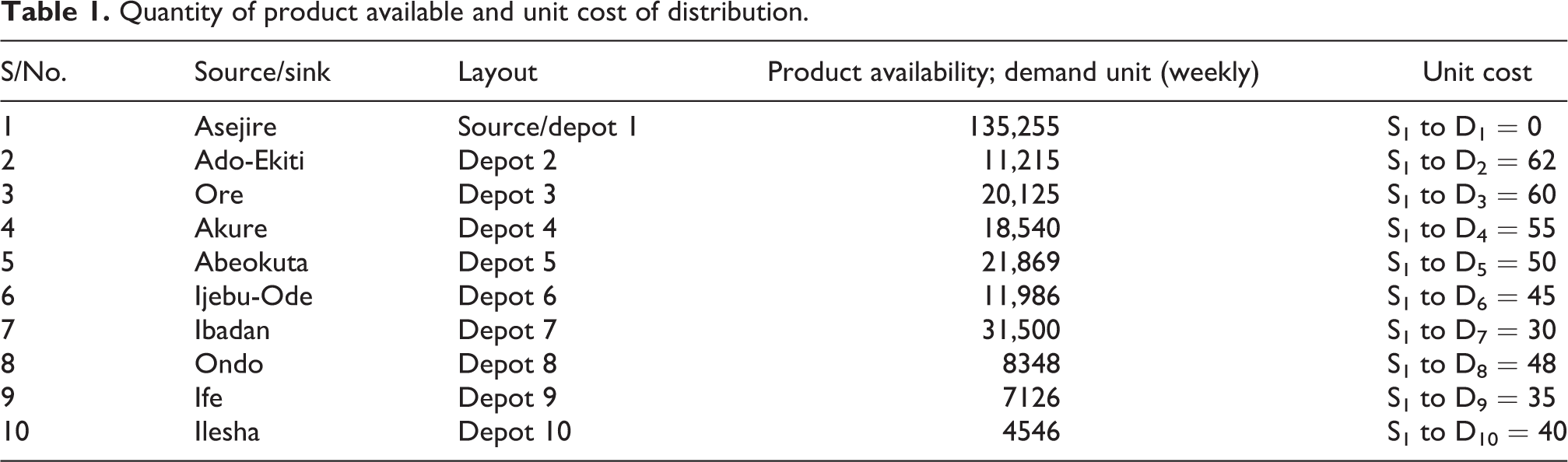
The company used as a case study is a multinational beverage bottling company with a single production plant, n = 1, a range of products represented by the single product family, i = 1, servicing the south western part of Nigeria and some neighboring cities via 10 depots, j = 10, and three TPs, k = 3, which also serve as depots. Data collected from the bottling plant are used for analysis. Matrices are developed for the distances, and the associated cost is as shown in Table 1. The current practice in the company is to ship directly to all depots from the plants, although they could have three TPs, D7, D9, and D10 selected through greedy heuristics, through which they could ship to the other depots as shown in Figure 2.

Table 1.

Quantity of product available and unit cost of distribution.

S/No.	Source/sink	Layout	Product availability; demand unit (weekly)	Unit cost
1	Asejire	Source/depot 1	135,255	S1 to D1 = 0
2	Ado-Ekiti	Depot 2	11,215	S1 to D2 = 62
3	Ore	Depot 3	20,125	S1 to D3 = 60
4	Akure	Depot 4	18,540	S1 to D4 = 55
5	Abeokuta	Depot 5	21,869	S1 to D5 = 50
6	Ijebu-Ode	Depot 6	11,986	S1 to D6 = 45
7	Ibadan	Depot 7	31,500	S1 to D7 = 30
8	Ondo	Depot 8	8348	S1 to D8 = 48
9	Ife	Depot 9	7126	S1 to D9 = 35
10	Ilesha	Depot 10	4546	S1 to D10 = 40

Figure 1.

Structure of the MATLAB ANN model. ANN: artificial neural network.

Figure 2.

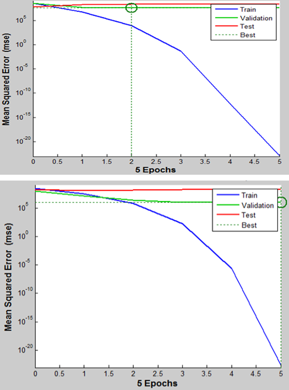
Rough and final MSE variations for training, testing, and validation data sets against epoch during the training. MSE: mean squared error.

Model implementation

The triangular functions were approximated by the deterministic equivalents (quantile values for the stochastic model and alpha cuts for the fuzzy model) to derive the training rules during implementation. The stochastic model is divided into quantiles of demand and cost value ranges from which the class values are used for determining the values required for ANN training process. The associated linguistic values for ANFIS model were defined, and different alpha cut values were defined using the fuzzy rules developed and the corresponding values of linguistic variables determined in consistence with the fuzzy decomposition theorems. ANN and ANFIS training of models were done using the derived values from the available data set.

In solving the transshipment problem where product flows from source through TPs for onward distribution to the final destination, the deterministic model was solved using Tora software 2.0. For the nondeterministic input variables problem, popular solvers were not useful. The ANN technique, using neural weight update algorithm, and the ANFIS technique, which works based on the principle of fuzzy inference rules, were used to determine the optimal weight vectors that minimize the objective function of the LP problem presented.

The ANFIS rule viewer is a simplified toolbox with inbuilt algorithms for both the fuzzification of input parameters and the optimization of neural weights inside the same toolbox. It presents the analyst with the input interface to specify the necessary fuzzy parameters for each variable involved and presents the output in a de-fuzzified manner once the appropriate de-fuzzification algorithm of choice has been specified.

The creative model

In implementing the ANN model, a feed-forward model with backpropagation, having 4-neuron input layer with linear combiner, 10-neuron middle layer, and a single-neuron output layer was designed using the sigmoid output transfer function. This is shown in Figure 1. The model is trained with the MATLAB ANN toolbox using the gradient descent algorithm. Mean squared error (MSE) was selected as the performance function, and R ² values were examined throughout the training period.

The following notations are defined for exclusive use within the ANN and ANFIS models.

U_k is the linear combiner output due to input signal

W_kv the connection weight from neuron v to neuron k

X_j the signal flow from source/input through synaptic weights to summing junction, that is, X ₁, X ₂, X ₃,…, X_j

j the index identifying the number of inputs

n the index identifying destinations

k the index identifying the processing elements

V_k the linear combiner with bias to support input signal

Y_k the total weighted sum of input to the kth processing element

p the index representing TPs (p = 1 for depot 7, p = 2 for depot 9, and p = 3 for depot 10)

W_ki the weight or strength of connection from neuron, i to k

X_ki the demand input signal from depots i to TPs k

η the learning rate of the neural network (NN) in the backpropagation algorithm implementation

A typical standard neuron consists of set of synapses, each characterized by weight or strength of connections. It also comprises the bias or summing junction and the activation junction. The total sum of the neuron $U_k$ is obtained by linearly combining all the inputs, multiplied by the appropriate weight or strength of connection so that in mathematical form, a neuron K is expressed as shown in the below equation

$U_k={\displaystyle \sum _{j=1}^n{x}_j}{w}_{kj}$

12

Rewriting equation (12) for each transshipment location (i.e. at each TP)

$U_{pk}={\displaystyle \sum _{j=1}^6{x}_j}{w}_{pkj}\forall p$

13

Introducing a bias (b_k ), then the combined input (V_k ) can be expressed as

$V_k={\displaystyle \sum _{p=1}^3{U}_{pk}}+bk$

14

Substituting the value of U_k for each p in equation (13) into equation (14), the combined input can be computed as

$V_k={\displaystyle \sum _{p=1}^3{\displaystyle \sum _{j=1}^6{x}_j}{w}_{pkj}}\forall p$

15

Defining the output threshold function as a sigmoid function $\varphi (.)= \frac{1}{1+e^{-\alpha x}}$ , then the total output can be expressed for each p, and with $W_{kn}$ from middle layer neuron k to output layer neuron n, equation (12) can be written as

$Y_{pk}=\varphi \left(w_{pkn}{x}_n+b_{pk}\right)= \frac{1}{1+ e^{-\Sigma w_{pkn}{x}_n+b_{pn}}}\forall p$

16

Batch update was done to train the neurons, and the general weight update rule for the NN is

$w_{\text{new}}= w_{\text{old}}- \eta \sum \delta x_j$

17

where $\delta =\left(Y_{\text{exp}.m}-Y_{\text{pred}}\right)$ when the transfer function is linear, $\delta =Y_{\text{pred}}\left(1-Y_{\text{pred}}\right)\left(Y_{\text{exp}}-Y_{\text{pred}}\right)$ when the transfer function is sigmoid, $Y_{\text{pred}}$ represents the predicted ANN value, and $Y_{\text{exp}}$ denotes the expected or targeted output value. According to Lotfan et al., ²⁴ equations (18) and (19) are used to test the fitness during training

$\text{MSE}=\frac{1}{n}{{\displaystyle \sum _{m=1}^n\left(Y_{\text{exp}.m}-Y_{\text{pred}.m}\right)}}^{\mathrm{ }}$

18

$R=\left(\frac{{\displaystyle {\sum }_{m=1}^n\left(Y_{\text{pred}.m}-y_{\text{pred}}\right)}\left(Y_{\text{exp}.m}-y_{\text{exp}}\right)}{\sqrt{{\displaystyle {\sum }_{m=1}^n{\left(Y_{\text{pred}.m}-y_{\text{pred}}\right)}^2{\displaystyle \sum _{m=1}^n{\left(Y_{\text{exp}.m}-y_{\text{exp}}\right)}^2}}}}\right)$

19

Data analysis, results, and discussion

Approach 1 (Using ANN)

Using a three-layer (input, hidden, and output) NN model as a result of the quantitative and architectural characteristics of the NN which has a close resemblance of the outbound manufacturing system where the input denotes product available at the source, and the route to different destinations represents weighted strength of the network. Table 2 shows the available data set for network training, with cost and demand set as input variables of W and X and the output which is the product availability, Y, at different TPs. D is the demand of products at various locations. In NN programming, it is necessary to train the network for accurate value. The accuracy of the value is a function of MSE and R values. Our goal is to minimize these errors. This was achieved by running series of iterations and training continuously with many weighted input parameters till a fairly minimal error is obtained.

Table 2.

ANFIS training data.

S/No.	Cost at TP7	Cost at TP9	Cost at TP10	D	YK 1	YK 2	YK 3
1	45	27	20	11,215	65,355	35,599	34,301
2	33	20	25	20,125
3	32	22	18	18,540
4	20	29	35	21,869
5	25	32	30	11,986
6	26	30	15	8348

ANFIS: adaptive neuro-fuzzy inference system; D: product demand; TP: transshipment point. Note: Y_{K 1} = product available at transshipment point 1; Y_{K 2} = product available at transshipment point 2; Y_{K 3} = product available at transshipment point 3.

Results and discussion

The goal of this section is to obtain the optimum cost of product distribution in a bottling system. The ANN was trained with four inputs, 10 hidden, and an output layer (4–10–1). The network was trained many times for effective evaluation of the accuracy of the model using MSE and R value to determine the degree of association between the predicted and expected values. The system of equation for MSE and R value is established in equations (18) and (19). Y _pred and Y _exp denote the predicted and experimental values obtained for the NN model, respectively. y _exp and y _pred also signify the average experimental and predicted values, correspondingly. The performance and best possible iteration result of the ANNs are presented in Table 1. Figure 4 presents testing performance with worthy MSE value of 1.57 × 10⁻⁵. Bold items in Table 3 also reveal good performance solution. Training and performance values of this network were obtained at 1.000 and 0.80369, respectively.

Figure 3.

Plot of ANN-predicted output against actual value for (a) training, (b) validation, (c) testing, and (d) target. ANN: artificial neural network.

Figure 4.

High-level fuzzy architecture for transshipment model.

Table 3.

Performance results of multilayer perceptron (MLP) network for different numbers of neurons in the hidden layer for testing data set.

		R value
No.	MSE	Training	Testing	Validation	Performance
1 (Rough)	6,514,260	0.9688	−0.9990	0.5950	0.37153
2	2,940,735	0.4768	−1.0000	1.0000	0.41513
3	3505	0.9994	−0.5558	−0.19681	0.63866
4	2800	1.0000	0.1035	−0.5057	0.69111
5	2851	1.0000	0.11657	0.80388	0.68865
6	3586	1.0000	0.10346	−0.5057	0.69111
7	3357	1.0000	−0.55358	0.71808	0.56428
8	2676	0.6810	0.4638	0.81260	0.65247
9	2280	0.9821	0.7218	0.56580	0.73260
10	1950	0.9784	0.7136	0.6842	0.71216
11 (Final)	1.57 × 10−5	1.0000	0.77089	0.95504	0.80369
12	78	0.9999	0.4447	0.67610	0.69830
13	1900	0.9998	0.6669	0.85110	0.78962
14	3839	0.9999	0.7134	0.82341	0.79990
15	2348	0.9999	0.7614	0.71320	0.68530

MSE: mean squared error, R: regression coefficient; R ²: average determination coefficient.

Figure 2(a) is the MSE value for rough iteration in which the best validation result was obtained at epoch 2 with the minimum MSE value of 65 × 10⁻⁵ (see Table 3, no. 1 in bold items).

In Figure 2(b), the training process was repeated for MSE and the best validation result was obtained at epoch 5 with minimum MSE of 1.57 × 10⁻⁵. This performance is meritorious compared to the MSE result obtained for rough iteration (see Table 3, no. 11 in bold items). Figure 5 shows the plots of the ANN-predicted outputs generated by the ANN model for training, validation, testing, and target. The performance value obtained is demonstrated in Table 4. A satisfactory iteration, though not hundred percent, is obtained in Table 4.

Figure 5.

ANFIS architecture with input–output membership functions. ANFIS: adaptive neuro-fuzzy inference system.

Table 4.

Performance value for ANN modeling (final iteration).

Results	Samples (%)	MSE	R
Training	68	1.56999 × 10−5	1.000000
Validation	16	—	0.955041
Testing	16	—	0.770892

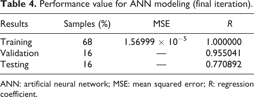
ANN: artificial neural network; MSE: mean squared error; R: regression coefficient.

Interpretation of the correlation coefficient (R)

The correlation coefficient specifies the degree of association or relationship among some variables of interest. Generally speaking, a correlation value of 0 is believed to be the absence of linear relationship, while 1 implies perfect relationsip between variables. There are rules for interpreting the R ² value, but a value greater than 0.7 and less than 1 can be regarded as substantial to meritorious for a reasonably sized data set.

Continuous iteration (or refining) of weight parameters was done to obtain a model with the best possible fit. The iteration was performed several times to obtain the best value as shown in Table 3 and Figure 3. Table 3 is a summary table showing the MSE and R values for the iterations. Apart from the 11th value in Table 3, other values have high MSE value for training, validation, and testing. The best solution to the programmed ANN system is obtained at the 11th run with the minimal MSE value. The ANN model at the first trial stage was trained with 50 data points of which the best 15 are shown in Table 3. This was done to test the effectiveness of the tool.

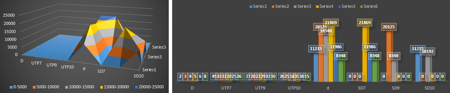
As shown in Figure 3(a) to (d), the R values for training, validation, and testing are: 1.000, 0.95504, and 0.77089, respectively, with performance value of 0.80369. Therefore, the ANN prediction for training, validation, and testing are substantial and meritorious in terms of correlation. The performance value for the final iteration gave a satisfactory result as shown clearly in Figure 9, where SD7 represents the Supply signal at D7; SD9 is the Supply signal at D9; SD10 is the Supply signal at D10; TP is the transshipment point; D is the product demand; UTP7 is the Unit cost from TP7 to depots; UTP9 is the Unit cost from TP9 to depots; UTP10 is the Unit cost from TP10 to depots; and D represents the Depots which are 10 in all.

Total cost of distribution at D7 = (45 × 0) + (33 × 0) + (32 × 0) + (20 × 21,869) + (25 × 11,986) + (26 × 0) = 737,030

Total cost of distribution at D9 = (27 × 8348) + (20 × 20,125) = 225,396 + 402,500 = 627,896

Total cost of distribution at D10 = (20 × 2867) + (18 × 18,540) + (15 × 8348) = 516,280

Total cost of transshipment = Supply cost at D7 + Supply cost at D9 + Supply cost at D10 = 737,030 + 627,896 + 516,280 = 1,881,206

Total cost of distribution in the entire system = Cost of distribution from source to TPs plus cost of distribution from TPs to final destination

$={\displaystyle \sum _{i=1}^n{\displaystyle \sum _{k=1}^m{C}_{ik}{X}_{ik}}}+{\displaystyle \sum _{k=1}^n{\displaystyle \sum _{j=1}^m{C}_{kj}{X}_{kj}}}=2,289,327+1,881,206=4,170,533$

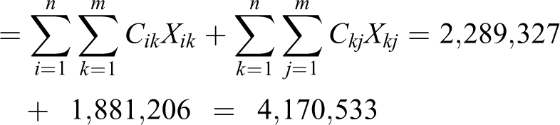
Therefore, total cost of distribution using the developed ANN model = 4,170,533.00

Approach 2 (Using ANFIS model)

In this section, fuzzy logic was used to find a delivery pattern that would meet customer demand and minimize delivery cost. Since there exists a source and 10 destinations with three possible TPs and there are two imprecise inputs, finding optimal solution requires continuous iterations. Using ANFIS, transshipment routes were created and analysis was carried out. Using the graphical user interface of Simulink to generate input, an initial fuzzy model was derived to trigger the modeling process. Membership functions were established for the input signals.

The high-level fuzzy model logic is shown in Figure 4. The input variables were passed into the fuzzy toolbox that utilizes the Sugeno class function for fuzzification. The membership functions (mf) at the input and output ends of the ANFIS logic were then defined so that the appropriate rules can be developed for training as shown in Figure 5. The triangular membership function (mf) was selected for the inputmf variables and the Gaussian for the outputmf supply signal. Examples of these can be seen in Figure 6(a) to (d). Figure 8 is an example of the three-dimensional (surface) views generated using the ANFIS rule viewer. Example of the application of the rule viewer using discretization of the continuous triangular inputs to take the relevant alpha cuts in order to generate the fuzzy inputs is shown in Figure 7. Eighty one training rules were developed. These rules are shown in the Appendix.

Figure 6.

Fuzzy Inference System (FIS) membership function plot for cost of distribution from TP7, TP9, and TP10 and demand at various destinations. TP: transshipment point.

Figure 7.

Rule viewer for input–output supply signals.

Figure 8.

Three-dimensional input–output surface plots.

Table 2 is the data set representing product demand at source and the available products at the TPs 7, 9, and 10 for onward distribution to the final destinations. Figure 8 shows the membership function plot for input variables in terms of demand.

The final allocation is presented in Figures 9 and 10, showing the quantity to be supplied from each TP to each of the destinations using ANN and ANFIS, respectively. It should be noted that each of the TPs supplied its own demands. The total distribution cost per week obtained (in Nigerian Naira, NGN) is shown in Figures 9 and 10. The solution produced using ANFIS is marginally cheaper than the one produced using ANN and the company’s traditional transshipment model. While the company’s traditional solution produced NGN6,332,304 minimum cost per week, ANN generated a minimum of NGN4,170,533. ANFIS, however, yielded a minimum cost of 4,053,661, which is better than both the traditional technique of the company and the ANN model solution.

Figure 9.

ANN solution figures for supply signal at TPs 7, 9, and 10. ANN: artificial neural network; TP: transshipment point.

Figure 10.

ANFIS optimal solution figures for supply signal at TPs 7, 9, and 10. ANFIS: adaptive neuro-fuzzy inference system; TP: transshipment point.

Total cost from TP to final destination = 1,764,334

Total cost of distribution from source to TPs = 2,289,327

Total cost of distribution in the entire system

$={\displaystyle \sum _{i=1}^n{\displaystyle \sum _{k=1}^m{C}_{ik}{X}_{ik}}+}{\displaystyle \sum _{k=1}^n{\displaystyle \sum _{j=1}^m{C}_{kj}{X}_{kj}}}=2,2\text{8}9,3\text{2}7+1,7\text{6}4,3\text{3}4=4,0\text{5}3,6\text{6}1$

Conclusion

In this article, ANN and ANFIS models have been applied successfully to solve a transshipment problem with nondeterministic demand and cost input variables. With data set obtained from a bottling company, training was performed using ANN fitting tool where the best iteration was considered based on MSE and R values obtained. The model based on the ANFIS logic was also implemented using the rule viewer interface. This model is capable of adjusting parameters based on series of alpha cuts taken on the data set. Our results seem to have followed the pattern reported in other papers that have compared the performance of models with nondeterministic inputs to those that used the mean values to approximate such variables. The results suggest that the ANFIS logic seems to have produced a slightly better solution than that obtained using the ANN, and both are much better than that obtained using the company’s traditional distribution algorithm. ANFIS is, however, only marginally better in this context, and it is generally inconclusive in the literature if one technique is better than the other.