Sage Journals: Discover world-class research

Abstract

In this article, we present the modeling of cutting performances in turning of 2017A aluminum alloy under four turning parameters: cutting speed, feed rate, depth of cut, and nose radius. The modeled performances include surface roughness, cutting forces, cutting temperature, material removal rate, cutting power, and specific cutting pressure. The experimental data were collected by conducting turning experiments on a computer numerically controlled lathe and by measuring the cutting performances with forces measuring chain, an infrared camera, and a roughness tester. The collected data were used to develop an artificial neural network that models the pre-cited cutting performances by following a specific methodology. The adequate network architecture was selected using three performance criteria: correlation coefficient (R ²), mean squared error (MSE), and average percentage error (APE). It was clearly seen that the selected network estimates the cutting performances in turning process with high accuracy: R ² > 99%, MSE < 0.3%, and APE < 6%.

Keywords

Turning surface roughness cutting forces cutting temperature material removal rate cutting power specific cutting pressure artificial neural networks

Introduction

Manufacturing processes can be classified into five principal types: shaping processes, property enhancing processes, surface processing operations, permanent joining processes, and mechanical fastening.¹ Shaping processes can be grouped into four categories: solidification processes, particulate processing, deformation processes, and material removal processes.¹

Machining is the most important category of material removal processes as it offers excellent dimensional tolerances and the best surface quality. However, machining processes tend to be wasteful as the material removed from the initial shape is waste, at least in terms of the unit operation.¹ Therefore, the most important task in these processes is to select the optimal combination of cutting parameters in order to achieve the required cutting performances² such as surface roughness, cutting forces, cutting temperature, material removal rate (MRR), power consumption, specific cutting pressure, and tool wear.

Machining can be defined as the process of removing excess material from an initial workpiece to produce the desired final geometry.¹ The workpiece is cut from a larger piece, which is available in a variety of standard shapes such as round bars, rectangular bars, round tubes, and so on. This material removal process includes three principal categories: turning, drilling, and milling.¹

Turning is one of the extensively used machining processes in industrial applications. It consists of removing material from an external or internal, cylindrical or conical surface.¹ The workpiece is rotated at a particular speed (cutting speed), and the cutting tool is fed against the workpiece (feed rate) at a certain level of engagement (depth of cut) as shown in Figure 1. Turning process can be conducted either on conventional lathe or on computer numerically controlled (CNC) lathe. Nowadays, the CNC lathe is widely used where machining operations are controlled by a program of instructions based on alphanumeric code. This machine tool provides more sophisticated and versatile means of control than mechanical devices.¹

Figure 1.

Basic turning operation.²

Surface roughness remains the main indicator of the machined workpiece quality and its dimensional precision. In fact, a low surface roughness improves several features of the machined product such as tribological properties, fatigue strength, corrosion resistance, and esthetical appeal. Consequently, the most important tasks in turning process are measurement and characterization of surface properties. There are different parameters to characterize the surface roughness.³ In this study, we selected the arithmetic average surface roughness (Ra) to characterize the surface roughness as it is a key requirement for many relevant applications in industry.

Cutting forces constitute representative data to characterize machining operations. They have to be known precisely in order to predict deflections on the machined part and optimize the industrialization of this part on the machines.⁴ In order to have true values of cutting forces, they have to be measured during cutting process which leads to costly trials. Consequently, there is a necessity to develop reliable models that predict these forces and investigate the effects of turning parameters on them.

In a turning operation, a considerable amount of the generated energy is largely converted into heat, which increases the temperature in the cutting area. This cutting temperature may cause several consequences such as (i) affecting the strength, hardness, wear resistance, and tool life; (ii) difficulty to control the accuracy of the machined piece due to its dimensional changes; and (iii) causing thermal damage to the workpiece and affect its properties and service life.⁵ Moreover, lower cutting temperatures cause pressure welding creating a built-up edge, while higher temperatures trigger oxidation and diffusion processes.⁶ Hence, the necessity of modeling the cutting temperature is of great prevalence.

MRR is the volume of material removed per minute. Higher value of this cutting performance is desired by the industry to satisfy the requirements of mass production without affecting the product quality. Higher MRR can be achieved by increasing the cutting parameters such us cutting speed, feed rate, and depth of cut. However, excessive cutting speeds may produce larger power, which may exceed the power available on the machine tool.⁷

Many parameters affect the cutting performances in turning process:

cutting conditions: cutting speed, feed rate, and depth of cut;

cutting tool geometry: nose radius, rake angle, side cutting edge angle, and cutting edge;

workpiece and tool material combination and their mechanical properties;

quality and type of the machine tool;

auxiliary tooling;

lubricant used;

vibrations between the workpiece, machine tool, and cutting tool.

The current article constitutes a considerable extension of our previous study,⁸ where we modeled the surface roughness in turning of AISI 1042 steel using the artificial neural networks (ANNs) approach. The developed network estimated this cutting performance with high accuracy (correlation coefficient (R ²) > 95%, mean squared error (MSE) < 0.1%, and average absolute error e < 10%). These relevant results have constituted a motivation to model additional cutting performances in turning process, for example, cutting forces, cutting temperature, MRR, cutting power, and specific cutting pressure using the same artificial intelligence technique. In order to realize this modeling, we used large and consistent data by conducting turning experiments on a CNC lathe under four turning parameters: cutting speed, feed rate, depth of cut, and nose radius and by measuring the cutting performances by forces measuring chain, roughness tester, and infrared (IR) camera. The developed network was evaluated by three performance criteria: R ², MSE, and average percentage error (APE).

In comparison to the previous studies conducted in this research field, the contributions of our study can be dressed as follows:

The developed model (ANN) can be efficiently exploited by researchers, industrials, and practitioners to estimate; at the same time, a set of eight cutting performances rather than using a model to estimate each performance as we found in the previous studies. In fact, each study evaluated only one or two cutting performances at most, while it is crucial to have information about a maximum number of cutting performances at the same time, as there are significant interactions between them and the cutting parameters. Indeed, the results of our previous study reveal that interactions between turning parameters have significant effects on surface roughness.⁹

The three main turning parameters considered in the previous studies were cutting speed, feed rate, and depth of cut. Unfortunately, few studies integrated the tool nose radius as a crucial cutting parameter in their modeling approaches. In fact, nose radius and its interaction with the three main cutting parameters have significant effects on surface roughness according to our previous study.⁹ Therefore, the integration of this parameter as an input of our ANN will contribute to take into account its main and interaction effects to model the eight cutting performances with high accuracy.

In this article, the second section presents a literature overview. In the third section, we will describe the experimental system. The fourth section is consecrated to detail the modeling approach followed by our study, while results and discussions are presented in the fifth section. Finally, the article concludes with conclusions and future work.

Literature review

A considerable number of research studies investigated the effects of cutting parameters on cutting performances.^10

–14 In addition, these studies developed models to estimate these performances by following various modeling approaches, such as the multiple regression modeling, mathematical modeling based on process’s physics, and artificial intelligence modeling.

Őzel et al.¹⁵ investigated the effects of feed rate, cutting speed, workpiece hardness, and cutting edge geometry on surface roughness and cutting forces in finish turning. The results revealed that the effect of cutting edge geometry on the surface roughness is remarkably significant. In addition, the authors concluded that the cutting forces are influenced not only by cutting conditions but also by the cutting edge geometry and workpiece surface hardness.

Kumar et al.¹⁶ investigated the effects of cutting speed and feed rate on surface roughness during turning of carbon alloy steels. Results revealed that surface roughness is directly influenced by the two studied parameters. Indeed, surface roughness increases with increased feed rate and it was higher at lower speeds and vice versa for all feed rates.

Thiele and Melkote¹⁷ conducted an experimental investigation of workpiece hardness and tool edge geometry effects on surface roughness in finish hard turning. They analyzed experimental results by an analysis of variance (ANOVA) to distinguish whether differences in surface quality for various runs were statistically important.

Aouici et al.¹⁸ compared the surface roughness obtained after machining of AISI H11 steels by ceramics and cubic boron nitride (CBN7020) cutting tools. Experiments were conducted according to Taguchi L₁₈ orthogonal array, and experimental data were used to develop multiple linear regression models for surface roughness prediction in respect of cutting speed, feed rate, and depth of cut. These models were validated by the response surface methodology (RSM) and the ANOVA. Moreover, these two tools were used to determine the effects of machining parameters, their contributions, their significances, and the optimal combination of these parameters that minimize surface roughness.

Effects of cutting parameters and various cutting fluid levels on surface roughness and tool wear in turning process were investigated by Debnath et al.¹⁹ Turning experiments were planed according to a Taguchi orthogonal array and carried out on mild steel bar using a TiCN + Al₂O₃ + TiN-coated carbide tool insert. Results of this study revealed that feed rate had the main influence on surface roughness (34.3% of contribution), followed by cutting fluid level (33.1% of contribution). For the tool wear, it was found that cutting speed and depth of cut were the dominant parameters influencing this cutting performance (43.1% and 35.8% of contribution, respectively). Authors determined also the optimum cutting parameters that lead to the desired surface roughness and tool wear.

Bensouilah et al.²⁰ studied the effects of cutting speed, feed rate, and depth of cut on surface roughness and cutting forces during hard turning of AISI D3 cold work tool steel with CC6050 and CC650 ceramic inserts. For both ceramics, a comparison of their wear evolution during time and its impact on surface quality was proposed. In addition, the study investigated the effects of cutting parameters on surface roughness and cutting forces and determined the levels of cutting regime that minimize these performances.

Azizi et al.²¹ investigated the influence of cutting parameters and workpiece hardness on surface roughness and cutting forces during machining of AISI 52100 steel with coated mixed ceramic tools. The authors demonstrated using the ANOVA that feed rate, workpiece hardness, and cutting speed have significant effects on surface roughness, while cutting forces are significantly influenced by depth of cut, workpiece hardness, and feed rate.

For cutting temperature, several studies have developed models to estimate this cutting performance in respect of different cutting parameters. Shihab et al.⁵ investigated the effect of cutting parameters (cutting speed, feed rate, and depth of cut) on cutting temperature during hard turning process. Significance of cutting parameters was investigated using statistical ANOVA, which indicated that the three cutting parameters have significant effects on cutting temperature. Results also revealed that within the investigated range, the cutting temperature is highly sensitive to cutting speed and feed rate. In addition, the study proposed a model to predict the cutting temperature and determined optimal values of cutting parameters using RSM.

Mia and Dhar²² proposed models to predict the average tool–workpiece interface temperature during hard turning of AISI 1060 steels. These models were developed using the RSM and ANN in respect of cutting speed, feed rate, and material hardness. In the RSM modeling, two quadratic equations of temperature were derived from experimental data. The ANOVA and mean absolute percentage error were performed to evaluate the adequacy of the developed models.

Experimental system

Material of workpieces and cutting tool

For the workpieces, 2017A aluminum alloy in the form of round bars with a diameter of 80 mm and a cutting length of 40 mm was used to conduct turning experiments. For the cutting tool, standard carbide tool inserts CNMG120404 and CNMG120408 were used for turning operations with nose radii of 0.4 mm and 0.8 mm, respectively.

Turning conditions and measurement

Turning experiments were performed on a CNC lathe in the Laboratory of Mechanical Manufacturing of ENSAM, Moulay Ismail University, Meknes, Morocco.

For each turning parameter, two levels were selected as we can notice in Table 1. The selection of levels took into consideration the material of both workpiece and cutting tool. The experiments were performed without cutting fluid.

Table 1.

Turning parameters and their levels.

		Levels
Parameters		Low	High
V	Cutting speed (m/min)	300	350
f	Feed rate (mm/rev)	0.2	0.4
a	Depth of cut (mm)	1.5	2
r	Nose radius (mm)	0.4	0.8

For the surface roughness measurement, the work surface was characterized by the arithmetic average surface roughness (Ra).³ After each turning operation, Ra was measured by a roughness tester, and the measurement was repeated thrice at different locations for each workpiece and average value was reported. Details of setting parameters of measure are as follows:

Cut-off length = 0.8 mm;

Cut-off number = 5;

Standard: ISO 4287;

Speed = 1 mm/s.

For the cutting forces measurement, we used a measuring chain formed by the following components:

Dynamometer Kistler 9129AA;

Multichannels Charge amplifier Kistler 5070A;

Data acquisition hardware 5697A;

DynoWare Software 2825D-02;

All necessary cabling.

During each turning experiment, cutting forces were measured by the dynamometer mounted below the cutting tool. Forces acting on the cutting tool were amplified by the multichannels charge amplifier, and the measured numerical values and graphics were stored in the computer using the data acquisition hardware and the DynoWare software already installed in the computer. The cutting forces were measured in three mutually perpendicular directions corresponding to:

passive force Fp (x-direction);

cutting force Fc (y-direction);

feed force Ff (z-direction).

For the cutting temperature measurement (T), we mounted an IR camera (Optris PI) on the machine tool and we connected it with the computer to get the cutting temperature during each turning experiment via the camera’s software. This IR method is best utilized as it un-interrupts turning process and data can be collected and analyzed at the same time.

For the MRR, cutting power (Pc), and specific cutting pressure (Ks), we computed their values for each turning experiment as follows:

MRR = f \times a \times V

P c = F c \times V

K s = \frac{F c}{a \times f}

Figure 2 summarizes the experimental system and procedure of each cutting performance measurement. By this experimental system, we conducted turning experiments with different combinations of turning parameters and their levels. We obtained a large data set of 48 experimental results, which can be exploited to model the cutting performances using the ANNs approach.

Figure 2.

Experimental system and cutting performances measurement.

Methods

In this study, ANNs approach was used to model the cutting performances in turning process in respect of turning parameters. They constitute a type of artificial intelligence techniques that emulate the biological connections between neurons.²³ These networks are able to replicate the same functions of human behavior, which are formed by a finite number of layers with different computing nodes called neurons. These latter are interconnected to form an ANN, and the organization of connections between neurons determines the type of the network and its objectives.²⁴ The processing ability of the network is stored in the interunit connection strengths called weights, which are adjusted during the training process using a training algorithm (or learning) so as to minimize a function of error between actual and desired outputs.²⁵ The most used function of error is the MSE. ANNs are efficiently exploited for modeling various problems due to their ability to model linear and nonlinear systems without the need to make assumptions implicitly as in most conventional statistical approaches. Currently, this artificial intelligence approach is extensively applied in various aspects of sciences, engineering, and technology: agricultural sciences,^26
–28 medicine,^29,30 business, management and accounting,^31,32 energy,^33
–35 environmental sciences,^36,37 chemical engineering,^38,39 engineering,^40

–43 and so one.

Based on their architectures, ANNs can be classified into two major categories: feed-forward networks and feedback networks.⁴⁴ The first category allows signals to travel only from input to output, and it is appropriate to model relationships between a set of input variables and one or more output variables. Feed-forward network is memoryless because the response of each layer does not affect that same layer.²³ The most commonly used family of feed-forward networks is the multilayers perceptron (MLP), where neurons are grouped into layers with connections absolutely in one sense from one layer to another.^23,24 In the feedback (or recurrent) networks, signals can travel in both directions by introducing loops in the network.²³ The neuron’s outputs are computed once a new input sample is introduced to the network⁴⁴ and the extracted computations from earlier input are fed back into the network, which provides a memory to the feedback networks. This type of networks is dynamic; its state is changing continuously until it achieves an equilibrium point and remains at this point until the presentation of a new input and a new equilibrium needs to be found.²⁴

Multilayers perceptron

The MLP network is a widely used type of feed-forward networks.²⁴ Figure 3 shows an MLP formed by an input layer, hidden layers, and an output layer. Neurons in input layer transfer the input variables x_i (i = 1,…, n) to neurons in the hidden layer. The following points describe the basic characteristics of an MLP network²³:

Each neuron in the network includes a nonlinear activation function that is differentiable.

The network is formed by one or more layers that are hidden from both the input and output neurons.

The network exhibits a high degree of connectivity, determined by the synaptic weights of connections between neurons.

Figure 3.

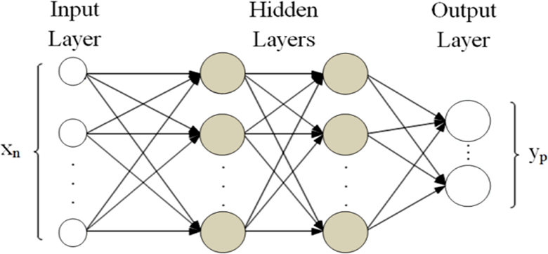
Multilayers perceptron network.⁸

The structure of an artificial neuron j (Figure 4) is characterized by

An addition function, which sums up the input signals x_i after weighting them with the weights of the respective connections w_ji from the input layer. The weighted sum S_j is given as follows:

S_{j} = \sum_{i = 1}^{n} w_{j i} x_{i}

An activation function f, which activates the neuron by the following equation:

y_{j} = f (\sum_{i = 1}^{n} w_{j i} x_{i} + b_{j})

Figure 4.

Structure of an artificial neuron.⁸

where b_j is the bias of neuron j.

The function f can also be called “transfer function” and can be linear, sigmoid, hyperbolic tangent, or radial basis function. The frequently used one is the sigmoid function, given as follows:

f (x) = \frac{1}{1 + exp (- x)}

Back-propagation algorithm

In order to adjust the weights of an ANN, we can exploit a training algorithm. In this context, the back-propagation algorithm is the most frequently used one for training the MLP networks.²³ The basic idea of this algorithm is defining an error function and use gradient descent to find a set of weights that optimize performance on a particular task.⁴⁵ The training process is carried out in two stages:

Forward stage

In this stage, the synaptic weights of connections between neurons are fixed and the input signal is propagated through the network’s layers until it attains the output layer. Hence, changes are limited to the activation potentials and neurons’ outputs in the network.^23,24

Backward stage

Once the forward stage is accomplished, an error signal is generated by comparing the network’s output and the required response. This error is propagated through the network’s layers in the backward direction. In this second stage, the synaptic weights of the network are subject to successive adjustments. These latter are simple for the output layer but more difficult for the hidden layers.^23
–25

Back-propagation algorithm includes several types: Levenberg–Marquardt algorithm, gradient descent algorithm, scaled conjugate gradient algorithm, one step secant, and resilient back-propagation algorithm.^23,46

Results and discussion

In this section, we will present the ANN that we developed to model the cutting performances in turning process. First, we will describe the methodology followed to choice the network’s architecture. Next, we will present the retained network, the steps of its development, and its performances. Finally, we will present the cutting performance models and the comparisons between their experimental and estimated values by the network.

For the network’s type, we selected an MLP network, which is a kind of feed-forward ANNs. It is widely used by researchers and it was noticed that this type trained with a back-propagation algorithm gave the most accurate results.^47,48

For the MLP’s architecture, we selected two architectures: (4-j-8) and (4-j-j-8). The first one is composed of three layers: one input layer for the four input parameters (cutting speed, feed rate, depth of cut, and nose radius), one hidden layer with j neurons, and one output layer for the eight outputs: surface roughness (Ra), cutting forces (Fp, Fc, and Ff), cutting temperature (T), MRR, cutting power (Pc), and specific cutting pressure (Ks). We selected this architecture because a three-layer feed-forward network with sigmoid hidden neurons and linear output neurons can fit multidimensional mapping problems arbitrarily well, if it is provided by consistent data and satisfactory number of neurons in its hidden layer.⁴⁹ The second architecture is the same as the first one except the number of hidden layers which is two for this architecture.

To ascertain the number j of neurons in the hidden layers, we followed the guidelines given by the study.⁵⁰ According to its authors, the recommended number of neurons in the hidden layer is n/2, 1n, 2n, and 2n+1, where n is the number of neurons in the input layer. Therefore, we developed eight networks with the following architectures:

One hidden layer: 4-2-8, 4-4-8, 4-8-8, 4-9-8.

Two hidden layers: 4-2-2-8, 4-4-4-8, 4-8-8-8, 4-9-9-8.

For the training process, we selected the Levenberg–Marquardt back-propagation algorithm,²³ which is a variation of Newton’s method designed to minimize functions that are sums of squares of other nonlinear functions.⁵¹ This characteristic makes this algorithm the adequate one to train our MLP network since the MSE is among the performance criteria to evaluate our developed network. Moreover, this algorithm is the most frequently used one as it guaranties faster training for networks of moderate size.^51,52

The eight networks were developed using the Neural Network Toolbox of MATLAB software. After the development, training, testing, and simulation of these networks, we determined their R ², MSE, and APE, and we recorded these performances criteria in Table 2. The best architecture must achieve the following performances: high R ², minimal MSE, and minimal APE. Therefore, the optimal architecture corresponds to (4-8-8) and it is detailed in Figure 5.

Table 2.

Performances of the developed networks.

MLP network	R ² (%)	MSE (%)	APE (%)
4-2-8	89.77	1.41	13.33
4-4-8	96.07	0.68	11.37
4-8-8	98.70	0.29	5.16
4-9-8	97.23	0.36	6.41
4-2-2-8	91.79	1.11	14.62
4-4-4-8	97.00	0.48	8.68
4-8-8-8	96.25	0.51	7.79
4-9-9-8	96.18	0.80	6.84

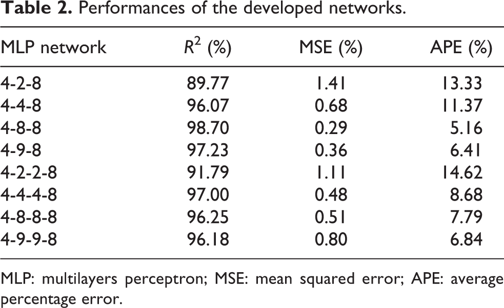
MLP: multilayers perceptron; MSE: mean squared error; APE: average percentage error.

Figure 5.

Architecture of the Multilayers perceptron (4-8-8).

The following steps describe in details the development of the retained network⁸:

Reading, randomization, and normalization of data

Before the creation of the MLP network, the program started by reading data (formed by 48 samples) from an Excel file, where each sample is defined by a combination of turning parameters (V, f, a, r) and the corresponding cutting performances (Ra, Fp, Fc, Ff, T, MRR, Pc, and Ks). Then, the data samples were randomized using the function “randperm” which returned a random permutation of samples, while the order of columns containing turning parameters and cutting performances for each sample was kept unchanged. After these two steps, data samples were normalized using the function “mapminmax” in order to equalize the importance of variables before introducing data to the network. Normalization of input and output variables was performed using their minimum and maximum values within a range of 0.1 and 0.9 as detailed below:

$x_{norm} = 0.8 \times \frac{x - x_{min}}{x_{max - x_{min}}} + 0.1$
7

where x _norm is the normalized value of a variable, x is real value of this variable, and x _max and x _min are the maximum and minimum values of x, respectively.

Creation of the network

After the normalization procedure, the network was created according to the parameters presented in Table 3.

Table 3.
Parameters of ANN process.

Network type Feed-forward back- propagation

Transfer function Hidden layer Sigmoid

Output layer Linear

Training algorithm Levenberg–Marquardt

Performance function MSE (goal = 10⁻⁴)

Data division Training data set 60% of the data

Validation data set 20% of the data

Test data set 20% of the data

Number of epochs 1000

Validation checks 100

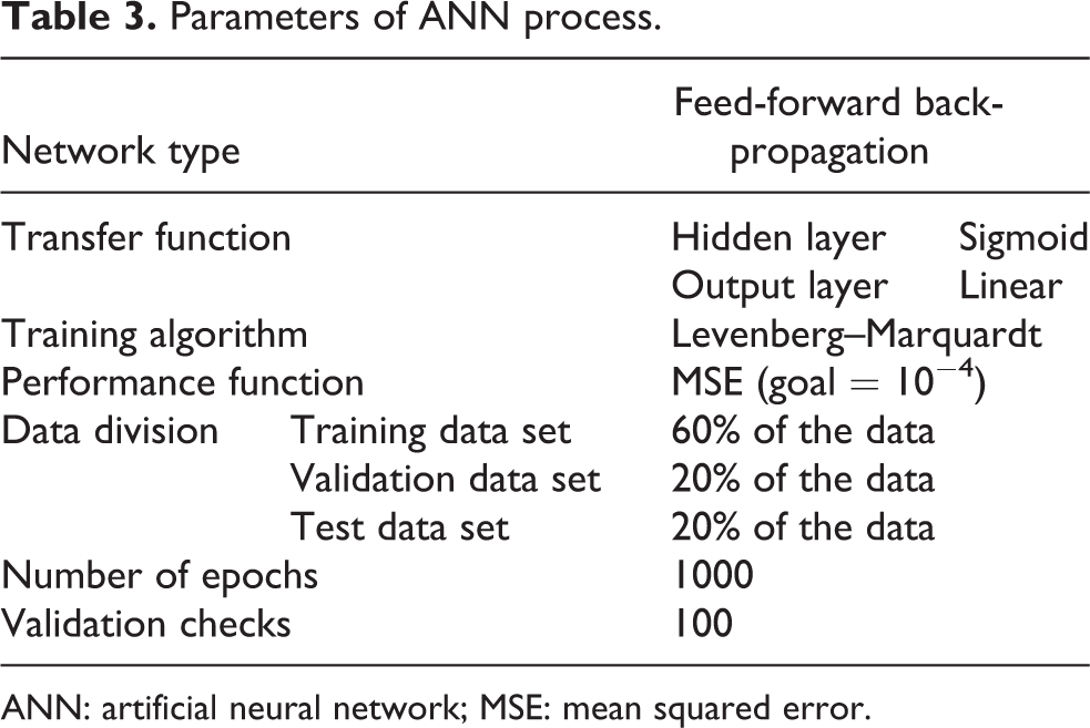
ANN: artificial neural network; MSE: mean squared error.

Training and testing of the network

From Table 3, we can remark that 30 samples were used to train the network, 09 samples for validation, and 09 samples were used to test the ability of the trained network to estimate the cutting performances. The training process was performed by adjusting the synaptic weights so as to minimize the MSE. A successful training was attained at epoch 168 with MSE = 0.29%, 100 validating checks, and R ² = 99.71%. The MSE performance plot for this network is shown in Figure 6.

Figure 6.
MSE performance plot of MLP (4-8-8). MSE: mean squared error; MLP: multilayers perceptron.

After the training stage, the developed network was tested with the experimental data that were not present in the training data set, in order to evaluate its ability to estimate the cutting performances. Performances of the network (4-8-8) in training and testing processes are detailed in Table 4 and Figure 7.

Table 4.
Performances of the MLP (4-8-8).

Performances Training data (%) Testing data (%)

R ² 99.71 96.42

MSE 0.04 0.50

MLP: multilayers perceptron; MSE: mean squared error.

Figure 7.
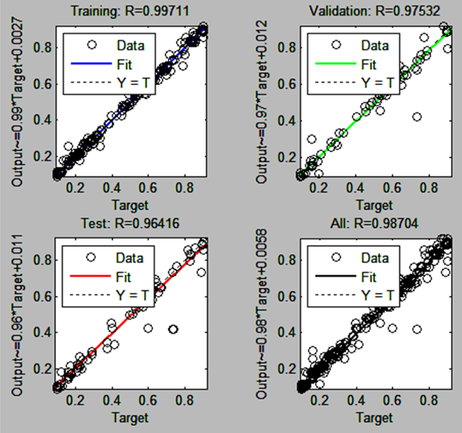
Regression plot for the multilayers perceptron (4-8-8).

In the hidden layer, neurons were activated by the “logistic-sigmoid” function. Equation (8) presents the activation of each neuron j:

$f_{j} = \frac{1}{1 + exp (- s_{j})}$
8

where s_j is the weighted sum of the normalized inputs (V, a, f, r) and it is calculated by equation (9). Weights w_ji and biases b_j for the eight neurons of the hidden layer are given in Table 5.

$s_{j} = w_{j 1} \times V + w_{j 2} \times f + w_{j 3} \times a + w_{j 4} \times r + b_{j}$
9

Table 5.
Weights and biases between input and hidden layer.

Neuron j w_j ₁ w_j ₂ w_j ₃ w_j ₄ b_j

1 −3.6982 3.2392 −3.6846 7.3188 −10.6536

2 −7.3398 −1.2854 −0.6287 −1.4340 7.9812

3 0.9469 6.3466 1.3403 −5.3478 −1.4537

4 −0.1547 −0.5303 −0.2526 0.0272 1.3210

5 −1.4451 2.7956 0.9360 −4.1080 3.8937

6 −9.6824 2.0989 3.2542 −2.6488 −5.1064

7 −1.3156 0.6428 −0.7512 0.7448 −1.3524

8 3.4567 −3.6575 −0.1875 −0.1682 0.4810

where V is the cutting speed, f is the feed rate, a is the depth of cut, and r is the nose radius.

In the output layer, neurons were activated by the “linear” function. Therefore, the normalized cutting performances which correspond to the output layer were computed by the following equations:

$\begin{array}{l} R a = 1.3498 f_{1} - 0.8870 f_{2} {+ 1.6374 f}_{3} {+ 2.2046 f}_{4} \\ + {1.0164 f}_{5} + 0.6978 f_{6} - 0.4589 f_{7} \\ + 1.0096 f_{8} - 3.2063 \end{array}$
10

$\begin{array}{l} F p = - 2.3126 f_{1} {- 0.9616 f}_{2} - 0.9212 f_{3} + {1.6950 f}_{4} \\ + {0.7079 f}_{5} - 1.6167 f_{6} + {1.1385 f}_{7} \\ - 3.4873 f_{8} + 1.7467 \end{array}$
11

$\begin{array}{l} F c = 0.1996 f_{1} {+ 0.2136 f}_{2} + {0.2351 f}_{3} {- 4.7126 f}_{4} \\ - 0.0046 f_{5} + 0.0232 f_{6} - 0.4971 f_{7} - 0.7072 f_{8} \\ + 3.7517 \end{array}$
12

$\begin{array}{l} F f = 0.9379 f_{1} {+ 0.5345 f}_{2} + {0.9624 f}_{3} {- 2.2443 f}_{4} \\ - 0.2178 f_{5} + {0.4693 f}_{6} - 1.8270 f_{7} - 0.2772 f_{8} \\ + 1.3119 \end{array}$
13

$\begin{array}{l} T = 1.2063 f_{1} {- 0.7646 f}_{2} - 1.5428 f_{3} {+ 5.4038 f}_{4} \\ - 0.6416 f_{5} - 0.4017 f_{6} - 6.2884 f_{7} - 5.2000 f_{8} \\ - 2.3496 \end{array}$
14

$\begin{array}{l} M R R = - 0.1173 f_{1} {- 0.0626 f}_{2} - 0.1314 f_{3} {- 6.5921 f}_{4} \\ + {0.0273 f}_{5} - 0.0562 f_{6} + {0.1704 f}_{7} - 0.1718 f_{8} \\ + 5.1059 \end{array}$
15

$\begin{array}{l} P c = 0.0363 f_{1} {+ 0.0818 f}_{2} + 0.1464 f_{3} {- 4.8787 f}_{4} \\ + {0.0826 f}_{5} - 0.1537 f_{6} - 0.2875 f_{7} - 0.4057 f_{8} \\ + 3.8083 \end{array}$
16

$\begin{array}{l} K s = 0.4395 f_{1} {+ 0.5360 f}_{2} + {1.1084 f}_{3} {+ 9.2143 f}_{4} \\ + {0.7163 f}_{5} - 0.5552 f_{6} - 1.5388 f_{7} - 0.6385 f_{8} \\ - 7.6368 \end{array}$
17

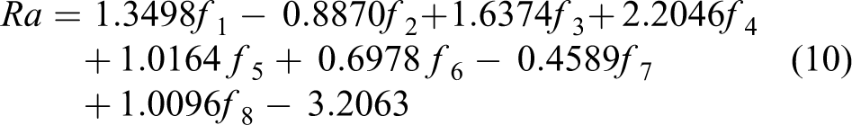
where f_j is the value of activation function for neuron j.

Simulation of the network

To compute the network’s outputs, we presented the whole normalized data to the developed network. Then, the obtained outputs were denormalized by the same function “mapminmax”(with the option “reverse”) in order to compare them with the experimental data. Comparison of experimental and estimated values of the eight cutting performances for the 48 experiments (training and testing data) is shown from Figures 8 to 15.

Figure 8.
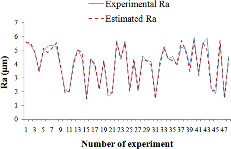
Comparison of experimental and estimated surface roughness.

Figure 9.
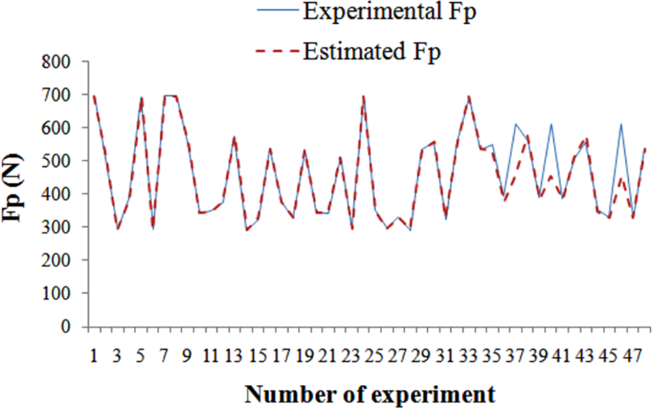
Comparison of experimental and estimated passive force.

Figure 10.
Comparison of experimental and estimated cutting force.

Figure 11.
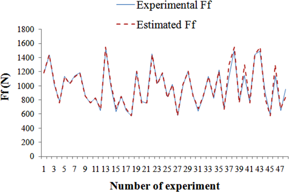
Comparison of experimental and estimated feed force.

Figure 12.
Comparison of experimental and estimated cutting temperature.

Figure 13.
Comparison of experimental and estimated material removal rate.

Figure 14.
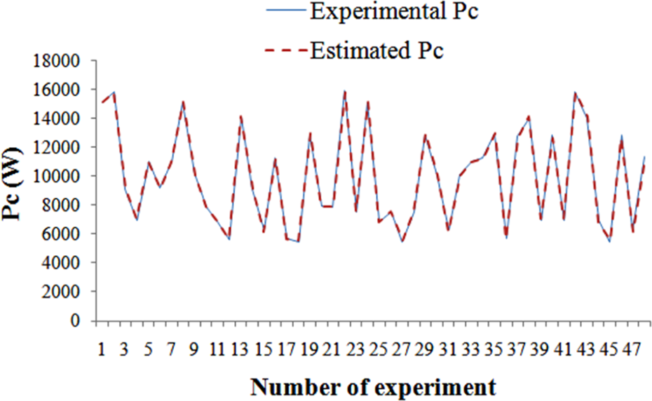
Comparison of experimental and estimated cutting power.

Figure 15.
Comparison of experimental and estimated specific cutting pressure.

According to these figures, there is a good agreement between the experimental and estimated values as the patterns of the two lines are identical for all cutting performances except the surface roughness Ra, the cutting force Fp, and the cutting temperature T, where few points show a difference between the two values. This is due to some errors caused by the measurements and other unknown factors. However, these points can be neglected as the R ² for training and testing data exceeded 95% and the APE for each response didn’t exceed 5.17% as we can see in Table 6. These relevant results confirm the ability of ANNs to estimate the eight cutting performances in turning process with high accuracy.

Table 6.
APE for cutting performances.

Model Ra Fp Fc Ff T MRR Pc Ks

APE (%) 5.17 2.35 0.74 2.51 1.49 0.88 0.82 0.43

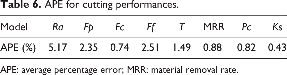
APE: average percentage error; MRR: material removal rate.

Conclusion

In this article, ANNs approach was used to model eight cutting performances (surface roughness, three cutting forces, cutting temperature, MRR, cutting power, and specific cutting pressure) in turning of 2017A aluminum alloy under four turning parameters: cutting speed, feed rate, depth of cut, and nose radius. Turning experiments were conducted on a CNC lathe. During each turning experiment, some cutting performances, for example, surface roughness, cutting forces, and cutting temperature, were measured by a roughness tester, forces measuring chain, and an IR camera, respectively, while the remaining performances were obtained directly from the measured ones. The collected experimental data were exploited to develop an ANN that estimates the pre-cited cutting performances.

To select the best architecture of the network, we followed a particular methodology that allowed us to develop eight MLPs networks and to choose the best one by three performance criteria: R ², MSE, and APE. The selected one corresponds to the MLP (4-8-8), trained by the Levenberg–Marquardt back-propagation algorithm and had the following performances: R ² = 99.71%, MSE = 0.29%, and APE = 5.17%.

From the developed network, we extracted a model for each cutting performance. Then, we plotted the comparison between experimental and estimated values for each response which revealed that there is a good agreement between the two patterns. Therefore, the ANNs are a reliable tool to model the cutting performances in turning process with high accuracy.

This article constitutes a considerable extension of our previous study,⁸ where we modeled just one cutting performance (surface roughness) in turning of AISI 1042 steel under the same turning parameters considered in the current study. This modeling was performed by exploiting the same artificial intelligence technique and the developed network estimated surface roughness with high accuracy (R ² > 95%, MSE < 0.1%, and APE < 10%). These interesting results have constituted a motivation to model additional cutting performances in turning process by following the same approach. Moreover, in comparison with our previous study, we followed a specific step to choose the number of neurons in the network’s hidden layer, which provided best results. Indeed, the APE decreased from 9.70% to 5.17% for the surface roughness estimation.

In comparison to the previous studies conducted in this research field, our study will contribute to estimate eight cutting performances at the same time instead of estimating each performance by its own model, which can be efficiently used by practitioners, industrials, and researchers. In addition, turning process is characterized by significant relationships either between cutting performances or between these performances and cutting parameters. This crucial point was taken into account by the followed approach as ANNs have the ability to learn these relationships. Moreover, our study integrated nose radius as turning parameter with the three main parameters considered in the previous studies, since the nose radius and its interaction with the other parameters have significant effects on cutting performances. Therefore, its integration contributes to estimate the cutting performances with high accuracy as we can conclude from results.

Practical implications

Concerning the practical implications, this study will provide to industrials practical information about the cutting performance values that they will attain with the considered turning parameters levels. In addition, the findings of this research will constitute a relevant technical database for several industrial applications of turning process, where industrials can exploit the developed model in optimization and decision-making stages in order to determine the optimal combination of turning parameters that lead to the highest cutting performances and improve the quality and the productivity of machining process. Moreover, due to its ability to learn complex linear and nonlinear relationships between cutting performances and turning parameters, the developed network can be integrated in-process and provide the possibility to understand, control, and take in time corrective actions to retain the cutting performances within the required limits.

Limitations of the study

The findings of this study are limited to the specified levels of turning parameters and the materials of workpieces and cutting tool. However, researchers and industrials interested by these results can follow the same approach, given in details in this article, in order to develop their own model using their own turning parameters levels, their selected materials, and the cutting performances that they want to model in turning process.

Future works

Considering the results and conclusions of this study, future directions and research works can be dressed as follows:
develop other models that could improve the accuracy for cutting performances estimation;

predict the optimal combination of turning parameters that optimize simultaneously the cutting performances;

include additional cutting parameters and performances that characterize the turning process;

integrate the developed model in simulation software to ensure that the final machined part corresponds to the required specifications and avoid the costs generated by rejected pieces;

follow the same methodology to model cutting performances in other machining processes.

Network type	Feed-forward back- propagation
Transfer function	Hidden layer	Sigmoid
Output layer	Linear
Training algorithm	Levenberg–Marquardt
Performance function	MSE (goal = 10⁻⁴)
Data division	Training data set	60% of the data
Validation data set	20% of the data
Test data set	20% of the data
Number of epochs	1000
Validation checks	100

Performances	Training data (%)	Testing data (%)
R ²	99.71	96.42
MSE	0.04	0.50

Neuron j	w_j ₁	w_j ₂	w_j ₃	w_j ₄	b_j
1	−3.6982	3.2392	−3.6846	7.3188	−10.6536
2	−7.3398	−1.2854	−0.6287	−1.4340	7.9812
3	0.9469	6.3466	1.3403	−5.3478	−1.4537
4	−0.1547	−0.5303	−0.2526	0.0272	1.3210
5	−1.4451	2.7956	0.9360	−4.1080	3.8937
6	−9.6824	2.0989	3.2542	−2.6488	−5.1064
7	−1.3156	0.6428	−0.7512	0.7448	−1.3524
8	3.4567	−3.6575	−0.1875	−0.1682	0.4810

Model	Ra	Fp	Fc	Ff	T	MRR	Pc	Ks
APE (%)	5.17	2.35	0.74	2.51	1.49	0.88	0.82	0.43

Footnotes

Declaration of conflicting interests

The author(s) declared no potential conflicts of interest with respect to the research, authorship, and/or publication of this article.

Funding

The author(s) disclosed receipt of the following financial support for the research, authorship, and/or publication of this article: This work was supported by the Laboratory of Computer-Aided Design and Manufacturing, ENSAM School, Moulay Ismail University, Meknes, Morocco.

References

Groover

. Fundamentals of modern manufacturing: materials, processes, and systems. 4th ed. New Jersey: John Wiley & Sons, 2010.

Yang

Tarng

. Design optimization of cutting parameters for turning operations based on the Taguchi method. J Mater Proc Technol 1998; 84: 122–129.

ISO 4287:1997. Geometrical Product Specifications (GPS)—Surface Texture: Profile Method—Terms, Definitions and Surface Texture Parameters. Geneva: International Organisation for Standardisation, 1997.

Dorlin

Fromentin

Costes

. Analysis and modelling of the contact radius effect on the cutting forces in cylindrical and face turning of Ti6Al4 V titanium alloy. Proc CIRP 2015; 31: 185–190.

Shihab

Khan

Mohammad

. RSM based study of cutting temperature during hard turning with multilayer coated carbide insert. Proc Mater Sci 2014; 6: 1233–1242.

Kopac

Sokovic

Dolinsek

. Tribology of coated tools in conventional and HSC machining. J Mater Proc Technol 2001; 118: 377–384.

Sahoo

Baral

Rout

. Multi-objective optimization and predictive modeling of surface roughness and material removal rate in turning using grey relational and regression analysis. Proc Eng 2012; 38: 1606–1627, 2012.

Dahbi

Ezzine

El Moussami

. Modeling of surface roughness in turning process by using artificial neural networks. In: Proceedings of the 3rd IEEE international conference on logistics operations management (GOL) (eds El Hilali Alaoui

Benadada

Boukachour

), Fez, Morocco, 23–25 May 2016, pp. 1–6. IEEE. DOI: 10.1109/GOL.2016.7731681.

Dahbi

El Moussami

Ezzine

. Multiple regression model for surface roughness using full factorial design. In: Proceedings of the 6th IEEE international conference on industrial engineering and systems management (IESM) (eds, Framinan

Perez Gonzalez

Artiba

), Seville, Spain, 21–23 October 2015, pp. 439–444. IEEE. DOI: 10.1109/IESM.2015.7380194.

10.

Chen

. Cutting forces and surface finish when machining medium hardness steel using CBN tools. Int J Mach Tools Manuf 2000; 40: 455–466.

11.

Darwish

. The impact of the tool material and the cutting parameters on surface roughness of supermet 718 nickel superalloy. J Mater Proc Technol 2000; 97: 10–18.

12.

Fang

Safi-Jahanshahi

. A new algorithm for developing a reference model for predicting surface roughness in finish machining of steels. Int J Product Res 1997; 35: 179–199.

13.

Kopač

Bahor

Soković

. Optimal machining parameters for achieving the desired surface roughness in fine turning of cold pre-formed steel work pieces. Int J Mach Tools Manuf 2002; 42: 707–716.

14.

Valera

Bhavsar

. Experimental investigation of surface roughness and power consumption in turning operation of EN 31 alloy steel. Proc Technol 2014; 14: 528–534.

15.

Őzel

Hsu

Zeren

. Effects of cutting edge geometry, work piece hardness, feed rate and cutting speed on surface roughness and forces in finish turning of hardened AISI H13 steel. Int J Adv Manuf Technol 2005; 25: 262–269.

16.

Kumar

Shetty

. Effect of spindle speed and feed rate on surface roughness of carbon steels in CNC turning. Proc Eng 2012; 38: 691–697.

17.

Thiele

Melkote

. Effect of cutting edge geometry and work piece hardness on surface generation in the finish hard turning of AISI 52100 steel. J Mater Proc Technol 1999; 94: 216–226.

18.

Aouici

Fnides

Elbah

. Surface roughness evaluation of various cutting materials in hard turning of AISI H11. Int J Indus Eng Comput 2016; 7: 339–352.

19.

Debnath

Reddy

. Influence of cutting fluid conditions and cutting parameters on surface roughness and tool wear in turning process using Taguchi method. Measurement 2016; 78: 111–119.

20.

Bensouilah

Aouici

Meddour

. Performance of coated and uncoated mixed ceramic tools in hard turning process. Measurement 2016; 82: 1–18.

21.

Azizi

Belhadi

Yallese

. Surface roughness and cutting forces modeling for optimization of machining condition in finish hard turning of AISI 52100 steel. J Mech Sci Technol 2012; 26: 4105–4114.

22.

Mia

Dhar

. Response surface and neural network based predictive models of cutting temperature in hard turning. J Adv Res 2016; 7: 1035–1044.

23.

Haykin

. Neural networks and learning machines. 3rd ed. New Jersey: Pearson Education, Inc., 2009.

24.

Dreyfus

Martinez

Samuelides

. Réseaux de Neurones: Méthodologie et Applications. 2nd ed, Paris: Eyrolles, 2004.

25.

Corriou

. Les Réseaux de Neurones Pour la Modélisation et la Conduite Des Procédés. Paris: Lavoisier Technique et Documentation, 1995.

26.

Ezzine

Lachhab

Eddahhak

. A methodology for identification of greenhouse humidity based on recurrent radial basis functions. Int J Math Stat 2011; 8: 17–24.

27.

de Oliveira

Leme

Barbosa

BHG

. A computer vision system for coffee beans classification based on computational intelligence techniques. J Food Eng 2016; 171: 22–27.

28.

Astray

Gullón

Labidi

. Comparison between developed models using response surface methodology (RSM) and artificial neural networks (ANNs) with the purpose to optimize oligosaccharide mixtures production from sugar beet pulp. Indus Crop Prod 2016; 92: 290–299.

29.

Weng

Huang

TCK

Han

. Disease prediction with different types of neural network classifiers. Telemat Inform 2016; 33: 277–292.

30.

Misiunas

Oztekin

Chen

. DEANN: A healthcare analytic methodology of data envelopment analysis and artificial neural networks for the prediction of organ recipient functional status. Omega 2016; 58: 46–54.

31.

Göçken

Özçalıcı

Boru

. Integrating metaheuristics and artificial neural networks for improved stock price prediction. Exp Syst Appl 2016; 44: 320–331.

32.

Namazi

Shokrolahi

Maharluie

. Detecting and ranking cash flow risk factors via artificial neural networks technique. J Bus Res 2016; 69: 1801–1806.

33.

Chine

Mellit

Lughi

. A novel fault diagnosis technique for photovoltaic systems based on artificial neural networks. Renew Energy 2016; 90: 501–512.

34.

Benedetti

Cesarotti

Introna

. Energy consumption control automation using Artificial Neural Networks and adaptive algorithms: Proposal of a new methodology and case study. Applied Energy 2016; 165: 60–71.

35.

Chiteka

Enweremadu

. Prediction of global horizontal solar irradiance in Zimbabwe using artificial neural networks. J Clean Prod 2016; 135: 701–711.

36.

Khademi

Jamal

Deshpande

. Predicting strength of recycled aggregate concrete using artificial neural network, adaptive neuro-fuzzy inference system and multiple linear regression. Int J Sust Built Environ 2016; 5: 355–369.

37.

Cheng

Wang

. Maximum burning rate and fixed carbon burnout efficiency of power coal blends predicted with back-propagation neural network models. Fuel 2016; 172: 170–177.

38.

Cao

Liu

Wang

. Modeling and simulation of VMD desalination process by ANN. Comput Chem Eng 2016; 84: 96–103.

39.

KhazaiePoul

Soleimani

Salahi

. Solubility prediction of disperse dyes in supercritical carbon dioxide and ethanol as co-solvent using neural network. Chin J Chem Eng 2016; 24: 491–498.

40.

Osarobo

Chika

. Neural network modeling for monitoring petroleum pipelines. Int J Eng Res Africa 2016; 26: 122–131.

41.

Veintimilla-Reyes

Cisneros

Vanegas

. Artificial neural networks applied to flow prediction: a use case for the Tomebamba river. Proc Eng 2016; 162: 153–161.

42.

Bhattathiri

Saraswathi

. ANN control of non-linear and unstable system and its implementation on inverted pendulum. Int J Curr Eng Technol 2014; 4: 826–831.

43.

Jalloh

Kyuro

Jalloh

. Integrating artificial neural networks and geostatistics for optimum 3D geological block modeling in mineral reserve estimation: a case study. Int J Min Sci Technol 2016; 26: 581–585.

44.

Jain

Mao

Mohiuddin

. Artificial neural networks: a tutorial. IEEE Comput 1996; 29: 31–44.

45.

Chauvin

Rumelhart

. Backpropagation: theory, architectures, and applications. New Jersey: Lawrence Erlbaum Associates, Publishers, 1995.

46.

Chabaa

Zeroual

Antari

. Identification and prediction of Internet traffic using artificial neural networks. J Intel Learn Syst Appl 2010; 2: 147–155.

47.

Rao

. C++, neural networks and fuzzy logic. New Delhi: BPB Publications, 1996.

48.

Zain

Haron

Sharif

. Prediction of surface roughness in the end milling machining using artificial neural network. Int J Exp Syst Appl 2010: 37: 1755–1768.

49.

Sukumar

Ramaiah

Nagarjuna

. Optimization and prediction of parameters in face milling of Al-6061 using Taguchi and ANN approach. Proc Eng 2014; 97: 365–371.

50.

Zhang

Patuwo

. Forecasting with artificial neural networks: the state of the art. Int J Forec 1998; 14: 35–62.

51.

Hagan

Demuth

Beale

. Neural network design. 2nd ed. Boston: PWS Publishing, 1996.

52.

Hagan

Menhaj

. Training feed-forward networks with the Marquardt algorithm. IEEE Trans Neural Netw 1994; 5: 989–993.

Modeling of cutting performances in turning process using artificial neural networks

Abstract

Keywords

Introduction

Literature review

Experimental system

Material of workpieces and cutting tool

Turning conditions and measurement

Methods

Multilayers perceptron

Back-propagation algorithm

Forward stage

Backward stage

Results and discussion

Reading, randomization, and normalization of data

Creation of the network

Training and testing of the network

Simulation of the network

Conclusion

Practical implications

Limitations of the study

Future works

Footnotes

Declaration of conflicting interests

Funding

References