Sage Journals: Discover world-class research

Abstract

In this article, we present a contribution to modeling, evaluation, and analysis of the inventory management systems performance and more generally stochastic discrete event systems with a batch behavior. For this contribution, we combine two models: the Supply Chain Operations Reference model, proposed by the Supply Chain Council, with the Batch Deterministic and Stochastic Petri Nets, which constitutes a very powerful dynamic modeling tool. To do this, we applied these tools on a typical model of inventory management system in order to show how the combination of these two tools can help us to model and analyze the performance of the inventory management system and to provide information on their behavior and the effects of their parameters. A resolution of the stochastic process associated with the warehouse management system will allow us to calculate the following performance indicators: average stock, average cost of stock, probability of an empty stock, and average supply and frequency. These indicators will help to monitor the activity of our stock management system, and therefore make the right decisions for the development of the organization.

Keywords

Modeling Stochastic Petri Nets inventory management systems SCOR model performance analysis

Introduction

Modeling, evaluation, and performance analysis of discrete event systems including production systems, storage systems, and especially the supply chain (SC) remain a major concern for different scientific communities and especially manufacturing ones.

Historically, research in modeling and performance evaluation had always involved two closely linked issues. In addition, we can clearly identify in practice a combination of performance assessment methods to certain modeling formalisms. The first works are based on the direct analysis of stochastic processes and more generally of Markov chains.^1

–4 The work of Jackson⁵ led, in the late of 50s, a new approach based on queuing networks. Other approaches have abandoned the formalism of queuing networks and adopt a new and more powerful formalism introduced in the early 60s. It is the Petri nets (PNs)^6
–8 formalism as basic form to which they added extensions ranging from simple timers constants⁹ until mechanisms more sophisticated such as stochastic Petri nets (SPNs),¹⁰ generalized stochastic Petri nets (GSPNs),^11,12 colored PNs,^13,14 and continuous PNs.¹⁵

In this article, we introduce the Batch Deterministic and Stochastic Petri Nets (BDSPNs) as a tool for modeling and performance evaluation of SCs. This model is developed by enhancing DSPNs¹⁶ with batch places and batch tokens.

The increasing complexity of logistics processes, the desire of a better configuration of various processes of SC, and the pursuit of multiple objectives¹⁷ (minimizing the costs and delays, maximizing service levels and profit …) make the study of SCs a complex task.¹⁸ Consequently, there is a need to use methods and effective modeling and analysis of these systems tools.

The objective of this article is to propose a modeling approach and evaluating the performance of a stock management system by combining two models: BDSPNs as a very powerful tool of modeling and the Supply Chain Operations Reference (SCOR) model, proposed by the Supply Chain Council (SCC).

SCOR is a modeling tool that defines an approach, processes, indicators, and best practices to represent, assess, and diagnose the SC.¹⁹

In this article, we will first show the interest of using BDSPNs and SCOR model for modeling, assessment, and inventory management systems performance analysis, which plays a major role in business-organized SCs. Second, we will present our model and inventory management system. Finally, we will present the performance indicators, calculated by a resolution of stochastic process associated with this system.

Research background

Batch Deterministic and Stochastic Petri Nets

Introduction

There are several classes of SPN models proposed for modeling and performance evaluation of SCs, such as SPNs, GSPNs,¹² and DSPNs.¹⁶ PNs introduced by Petri (1962), as a graphical and mathematical tool, but not be used for modeling and analyzing complex systems which can be characterized as deterministic and/or stochastic.^20
–22 SPNs emerged as a modeling formalism for performance analysis in the early 1980s. In an SPNs, it associates an exponentially distributed delay with the firing of each transition.^23,24 GSPN is an extension for SPN, with two additional modeling elements: immediate transitions and inhibition arcs.^12,25 A DSPN is an extension for GSPN, which adds deterministically timed transitions.¹⁶

In this section, we will introduce the BDSPNs as a new class of SPNs, which is an extension of DSPNs by introducing batch places and batch tokens. Systems such as SCs, purchasing, production, and distribution are usually performed in a batch way with customer orders playing an important role, which justify the motivation for using the BDSPNs. In this last, we can distinguish between two types of places: discrete places and batch places. For the discrete places, tokens (which are the same as those in standard PNs) are viewed indifferently, while tokens in a batch places (which have sizes) are viewed as different individuals, called batch tokens.²⁶

BDSPNs are characterized by:

They may have inhibitor arcs and marking-dependent weights of arcs.

If a transition has an inhibitor arc, it is enabled only if the number of tokens in the input place of the arc is less than the weight of the arc and the firing of the transition does not remove any token from the place.

They have three types of transitions: immediate transitions, deterministically timed transitions, and stochastic transitions with exponentially distributed firing time.

For an immediate transition, tokens will be created in their output places as soon as it is fired, while tokens will be created either after a deterministic time or a time randomly generated according to an exponential distribution.

The transition firing conditions and the state evaluation of BDSPNs are similar to those of DSPNs except in BDSPNs where the transitions may be fired in a “batch” way when batch tokens are involved.

Performance evaluation

The performance evaluation is based on the temporal evolution of the model μ-marking process.^26,27 Two main approaches may be possible in the case of deterministic and stochastic Petri networks batches:

An analytical approach based on the graph of μ-markings used in conjunction with stochastic processes in order to benefit from the evaluation methods of stochastic processes. This approach is particularly applicable in the case where the network generates a finite number of states (μ-marking);

An approach based on discrete event simulation. This technique is particularly useful in the case where the system is too complex for analytical study or when the number of states generated by the model is infinite.

In our study, we applied the analytical approach to evaluate analytically the performance of our system modeled by the BDSPN model. Indeed, the general procedure is given by the algorithm described in Table 1. ²⁶

Table 1.

Algorithm of the general procedure of analysis for the evaluation of performance.

Step	Description
1	Construct the graph of μ-markings. The set of nodes (states) of the graph is the set of μ-accessible BDSPN markings. Every state is connected to its successor states by directed arcs. Each arc is labeled with the crossed transition. Batches transitions are marked by their crossing indices batches (t_j _[q]).
2	Eliminate the unstable states, arcs, and the corresponding immediate transitions in the obtained graph of μ-markings. This step generates the graph of μ-markings named reduced.
3	The stochastic process noted by {µ(t), t ≥ 0} is the graph of the reduced μ-markings. Space of states S = {s_i }; the resulting of the stochastic process is the set of reachable μ-markings of the BDSPN (µ_i = s_i ). The transition rates between the states of the stochastic process correspond to those of crossed transitions.
4	Characterization and study of the associated stochastic process. Determination of the stationary distribution of the process states probabilities using the methods of solving stochastic process depending on its nature.
5	By knowing the stationary probability distribution of states of the process, it is possible to evaluate the quantitative performance indices that characterize the BDSPN modeled system.

BDSPN: Batch Deterministic and Stochastic Petri Net.

To calculate the indices of performance of a BDSPN, it is necessary to calculate the state probabilities in permanent regime, that is to say, the probability of being in a specific μ-marking. For this calculation, the BDSPN must be limited, and its graph of μ-marking has a finite state space. The type of the resulting stochastic process must be identified in order to be resolved by an appropriate method appropriated to the nature of this process. Thus, the resolution of the latter determines the stationary distribution of probabilities π_i of states s_i which allows the evaluation of performance indices of the modeled system.

In general, if r(µ) represents an “index” function, then the index mean is:

P_{Moy} = \sum_{i / µ_{i} \in G µ A (BDSPN, µ_{0})} r (µ_{i}) \times π_{i}

Unlike other class of stochastic Petri networks, BDSPNs can capture the performance metrics that characterize their two types of components: batch and discrete components.

Performance indicators relative to batches components are:

The average number NL of batch tokens in a batch place p ∊ Pb is given by:

NL {(p)}_{Moy} = \sum_{i / µ_{i} \in G µ A (BDSPN, µ_{0})} Card (µ_{i} (p)) \times π_{i}

where Card(µ_i ) is the number of batch tokens available in the p at µ_i state, and Pb means all batches places.

The average number NL(b, p) of batch tokens with size equal to b in a batch place p ∊ Pb is given by:

NL {(b, p)}_{Moy} = \sum_{i / µ_{i} \in G µ A (BDSPN, µ_{0}) µ_{i} (p) = b} Card (µ_{i} (p)) \times π_{i}

where Cardb(µ_i ) is the number of batches tokens with size equal to b available in the place p at µ_i state.

The average sum of the sizes of batches tokens of a batch place p ∊ Pb corresponding to the average M-marking M(p) _Moy of this place is given by:

M {(p)}_{Moy} = \sum_{i / µ_{i} \in G µ A (BDSPN, µ_{0}) (\sum_{b \in µ_{i} (p)} b) \times π_{i}}

Let S(t_j _[q]) be set of μ-marking in the graph GµA(BDSPN, µ ₀), where the batch transition t_j is crossed by a batch crossing index q. The average frequency of crossing t_j _[q] is given by:

F {(t_{j [q]})}_{Moy} = \sum_{µ_{i} \in S (t_{j [q]})} λ_{j [q]} \times π_{i}

Modeling of inventory management systems

Whatever the activity of the company, its size, and its organization, stocks exist. Free production stock is almost inconceivable given the many functions performed by stocks.²⁸ The competitiveness of the company can be particularly affected by its inventory management,^29,30 which constitutes a sufficient reason to pay close attention. Indeed, stockpiling is necessary for many strategic and operational reasons. Supply means ensuring delivery of programming needs and inventory as part of the general planning of the company. Define a supply policy consists essentially on answering three questions:

WHAT (what product) should you supply?

WHEN should you supply it?

HOW should you supply?

In theory, any combination of answers to these three questions determines an inventory management policy that could be adopted for the management of a particular item.

In practice, some combinations have advantages over others and are therefore needed more frequently. In particular, policies identified as the most used in practice inventory management are described in Table 2.

Table 2.

Most used policies in practice inventory management.

Policy	Description
(s, S)	In this policy, as soon as the stock level falls below a threshold s, a supply order stock increased immediately to try to bring the stock level to its original level S.
(R, S)	In this policy, each R time units, a procurement order stock increased to try to bring the stock level to its original level S.
(R, s, S)	In this policy, each R units of time, the stock level is checked and if it is below a threshold s, a supply order stock increased to try to bring the level of its stock initial level S.
(s, Q)	In this policy, as soon as the stock level is below a threshold s, a procurement order of a fixed quantity Q has passed.
(R, s, Q)	In this policy, each R units of time, the stock level is checked and if it is below a threshold s, a supply control of a fixed quantity Q is increased.
(S − 1, S)	This is a special case of the policy (s, S) with s = S − 1 and a continuous monitoring of stock levels.

It is obvious that each policy is adapted to a product or product category. This often leads companies to use these policies simultaneously. The challenge is to choose the best policy for every product that prevents stock-outs without significant financial asset. Each procurement policy has its advantages and disadvantages. As advantage, we particularly appreciate the simplicity of the procedure, while for disadvantages, it will highlight the costs of the proceedings and especially the risk of possible break. Therefore, each method is ensuring that the disadvantages of this method are acceptable for the company.^28,31,32

Having chosen one of the policies described above, there has yet to set the parameter values that define the system (i.e. the values of s, S, R, and Q) so as to minimize the cost function in question. This optimization problem is generally complex, and thus, it is solved by using heuristic methods.³³

In this work, we are interested in modeling a stock management system in an automotive wiring business, with model based on a stock management policy with continuous review (s, S). The BDSPN model in Figure 1 models a stock managed by the policy (s, S), with ongoing review.

Figure 1.

BDSPN model management policy (s, S). BDSPN: Batch Deterministic and Stochastic Petri Net.

In this model, the stock is modeled by the place p ₁ and level of p ₁ stock, M p ₁ plus supply current orders, and M p ₃ is modeled by the place p ₂.

The output of the stock is modeled by the transition t ₁ that we have seen exponential in these representations. It describes customer demand following a Poisson process. t ₃ transition models the operation of the award of procurement orders from stock and t ₂ transition models the supply operation of the stock. t ₃ transition is immediate (crossing time is 0), which specifies that the revision of the stock is continuous.

In other words, the award of procurement orders is done immediately when the stock status is considered critical. Holding the stock is ensured thanks to the following:

Place p ₂ photographing with his M-marking M(p ₂), the level of stock M(p ₁), and supply current orders M(p ₃).

The arc inhibitor is combined to place p ₂ whose weight corresponds to the threshold of a supply order. It thus controls the level of inventory, M(p ₂), p ₁ stock.

t ₃ transition and its corresponding arcs modeling model triggering procurement order. The weight associated with these arcs corresponds to the quantity of the command to execute depending on the modeled policy.

SCOR model

Review of SCOR model

Every business process has different characteristics. Thus, a good understanding of the SCM processes is necessary before developing a simulation model.³⁴ In the past, different metrics were used to measure performance at different SC levels, and models for decision-making at strategic level were scarce.³⁵ It is not achievable to have a model that perfectly represents SCM but a closely adapted model^36,37 SCOR is achievable. In 1996, the SCC has developed and released a structured framework model SCOR for SCM systems and practices.³⁸ SCOR model is the first cross-industry framework for evaluating and improving SC performance and management.^35,39 The benefit of the SCOR model is the provision of a standard format and a comprehensive methodology to facilitate communication and to improve SC operations.^36,40 In order to achieve the desired performance in the internal and external levels, upper management of a company is highly recommended to use SCOR to design and reconfigure its SC, as it constitutes a common language and a flexible framework.³⁵SCOR is widely used in academia and practice. For these reasons, we use the SCOR framework as a base of our analysis.

SCOR is a business process framework that spans from the supplier’s supplier to the customer’s customer.¹⁹ SCOR 11.0 describes an SC by four levels of details. Level 1 is a top level that defines the scope and high-level configuration by six core processes, that is, plan, source, make, deliver, return, and enable. Level 2 is a configuration level and processes at this level, along with their positioning, determine the SC strategy. Level 3 is a process element level and describes the steps that need to be performed to execute all the processes of the level 2. Level 4 is the implementation level and describes industry-specific activities that are required to perform level 3 processes.

For the SCOR’s components, each one constitutes an important intraorganizational function and a critical interorganization process.⁴¹

SCOR core processes are defined below and shown in Figure 2. ¹⁹ The process reference model utilized in our research is based on SCOR 11.0.

Figure 2.

SCOR model.

SCOR sourcing process

The sourcing processes are critical to many industrial companies. The industrial company is looking for this process to expect deliveries (receiving, inspection, storage/transfer payment); to identify and select its sources, to define and organize the supply management rules (both in terms of evaluation of supplier performance as maintenance supplies data); and to manage its product arrivals, stocks, infrastructure network providers, export–import constraints, and supplier contracts.

The sourcing processes at level 2 include source stocked product (S1), source make-to-order product (S2), and source engineer-to-order product (S3). There are 17 process elements at level 3, including S1.1, S1.2, S1.3, S1.4, S1.5, S2.2, S2.3, S2.4, S2.5, S3.1, S3.2, S3.3, S3.4, S3.5, S3.6, and S3.7.

This research selects level 2 of the SCOR sourcing process “source make-to-order product (S2)” to modeling, evaluation, and analysis of the performance of our inventory management systems.

The detailed codes of the SCOR sourcing processes source make-to-order product (S2) at level 3 are as follows:

Schedule product deliveries S2.1

Receive product S2.2

Verify product S2.3

Transfer product S2.4

Authorize supplier payment S2.4

Table 3 shows the performance metric codes of the SCOR sourcing processes source make-to-order product (S2) at level 2; there are 17 performance metrics for this level.

Table 3.

Performance metric definition of SCOR sourcing “make-to-order product” process at level 2.

Attribute	Metric code	Metrics
Reliability	RL.1.1	Perfect order fulfillment
Responsiveness	RS.1.1	Order fulfillment cycle time
Responsiveness	RS.2.1	Source cycle time
Flexibility	AG.3.9	Additional source volumes obtained in 30 days
	AG.3.40	Current purchase order cycle times
	AG.3.42	Current source volume
	AG.3.46	Demand sourcing-supplier constraints
Cost	CO.2.002	Sourcing cost
	CO.3.005	Sourcing labor cost
	CO.3.006	Sourcing automation cost
	CO.3.007	Sourcing property, plant and equipment cost
	CO.3.008	Sourcing GRC, inventory and overhead cost
	CO.2.003	Material landed cost
	CO.3.009	Purchased materials cost
	CO.3.010	Material transportation cost
	CO.3.011	Material customs, duties, taxes, and tariffs cost
	CO.3.012	Material risk and compliance cost
Asset	AM.1.2	Return on supply chain fixed assets
	AM.1.3	Return on working capital
	AM.2.3	Days payable outstanding
	AM.3.16	Inventory days of supply – raw material

SCOR: Supply Chain Operations Reference; GRC: Governance, Risk, Compliance.

After defining performance indicators sourcing processes source make-to-order product (S2) established by the model SCOR, we modeled, analyzed, and assessed some of these indicators based on the dynamic model BDSPNs through a case study presented in the next section.

Case study

In this section, an analytical study is presented on a stock management system modeled by a BDSPN. This study is based on the graph of BDSPN μ-markings used in conjunction with the associated stochastic process. The resolution of the stochastic process used to determine the probabilities of the various states and the use of these probabilities assesses the average performance of the system.

The BDSPN model of this system is limited (finite state) and shows no mathematical constraints for the characterization and study of the associated stochastic process.

System description

The storage system considered in this study is shown in Figure 3 and has the following characteristics:

Figure 3.

Description of the storage system to study.

The stock is managed by the policy (s, S) with continuous review.

The stock of the raw material is modeled by p ₁ instead.

The production hall is modeled by a set comprising: t ₁: ready production orders; p ₅: production orders in process; p ₄: products required to produce a batch depending on the size of the production order; and t ₄: production operation.

Orders productions are in a batch mode. They are generated by following different sizes.

The lead time of the stock is stochastic. It follows an exponential law.

Orders productions (batches) arrive via the transition t ₄ and begin waiting in the lot instead p ₆.

Modeling system

The storage system to be studied is modeled by the BDSPN in Figure 4. The input and output of the stock instead modeled by p ₁ are represented by t ₁ and t ₂ transitions, respectively. The stock is managed by the policy (s, S) with continuous revision.

Figure 4.

BDSPN model of the storage system to study.

Recall, it is to inspect the stock level continuously and when it falls to a predetermined level s (weight of inhibitor arc from p ₂ to t ₃), a supply control of the stock is on to try to recomplete the stock at a level set at S.⁴²

The size of the procurement order is determined by the variable weight, S − M(p ₂), the arc connecting p ₃ to t ₃. The stock, p ₁, is subject to random requests for uses by the production workshop and sizes. Requests for applications are randomly generated by the transition t ₁ lot following a Poisson process of rate λ ₁. The transition t ₁ is exponential since in a Poisson process, the interarrival dates are distributed exponentially.

If the stock is available, the execution of a request of use is by crossing the batch transition t ₁. Crossing at a time t ₁ decreases the M-marking p ₁ site (stock) and that of p ₂ (representing the position of the stock, M(p ₂) = M(p ₁) + M(p ₃)) up a lot amount of size equal to the size of the production order to produce.

Once the stock level (M-marking p ₂) falls below the thresholds, monitored by the inhibitor arc connecting the transition t ₃ in the place p ₂, a supply order is immediately passed with the crossing of the immediate transition t ₃ (continued inspection of stock). Crossing the transition t ₃ adds in order with quantity (batch) of S − M(p ₂) in the batch place p ₃. This batch place represents the supply orders in execution waiting in order to attempt to bring back the level of stock to S.

The supply operation is executed by crossing the transition t ₂ whose crossing delay times are exponentially distributed.

The parameters of the policy management of the stock (s, S) are fixed to (2, 4). We consider that there are only two possible sizes (1 or 2) concerning production orders, where the μ-marking of batch place p ₆, modeling the production orders in expectations, is µ(p ₆) = {1, 2}.

The initial μ-marking is: µ ₀ = (4, 4, Ø, 0, Ø, {1, 2}).

Evolution of the modeled system

The evolution of the system can be expressed by using the graph of μ-markings BDSPN model that represents this system.

Each μ-marking of the graph represents the state of the system and each crossing between two μ-markings in the graph represents the execution of an operation that can be the award of a supply (crossing t ₃) and supply stock (crossing t ₂).

The graph of μ-markings of BDSPN is shown in Figure 5. This graph is built from the initial μ-marking µ ₀ considering all possible crossings of a μ-marking to another. To recall, the immediate transitions are prior than timed transitions. The resulting graph contains 15 tangible states numbered from 0 to 14.

Figure 5.

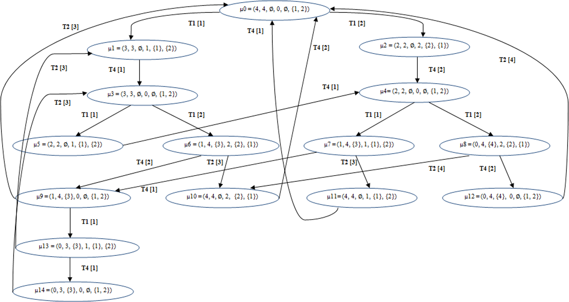
μ-Markings graph model.

The μ-marking graph generated by the BDSPN of the modeled system is isomorphic to a continuous time Markov chain shown in Figure 6.^2,3 The nature of the stochastic process generated is verified by the nature of distribution laws associated with the transitions used (without memory law).

Figure 6.

The Markov chain associated.

In other words, during the evolution of the model, only the new μ-marking determines the future behavior of the stochastic process.

Resolution of the associated stochastic process

For the rest of the study of this system, we will be limited to the following case: λ ₁[1] = λ ₁[2] = λ ₁ and λ ₃[3] = λ ₃[4] = λ ₃.

λ ₁[1] = λ ₁[2] = λ ₁: means that the arrival of the two types of production orders follows two exponential laws of identical parameters.

λ ₃[3] = λ₃[4] = λ ₃: means that the supply delay times don’t depend on the size of the supply orders.

t ₄ transition is exponentially distributed with a parameter #λ ₂. The symbol # indicates that λ ₂ parameter of the transition t ₄ depends on the size of the batch that crosses this transition: λ ₂[2] = λ ₂ means that λ ₂[1] = 2λ ₂.

In this case, the generator of the Markov process Q (transition matrix) associated with the stochastic μ-markings process is given in Table 4.

Table 4.

Transition matrix.

		µ ₀	µ ₁	µ ₂	µ ₃	µ ₄	µ ₅	µ ₆	µ ₇	µ ₈	µ ₉	µ ₁₀	µ ₁₁	µ ₁₂	µ ₁₃	µ ₁₄
Q	µ ₀	−2λ ₁	λ ₁	λ ₁	0	0	0	0	0	0	0	0	0	0	0	0
	µ ₁	0	−2λ ₂	0	2λ ₂	0	0	0	0	0	0	0	0	0	0	0
	µ ₂	0	0	−λ ₂	0	λ ₂	0	0	0	0	0	0	0	0	0	0
	µ ₃	0	0	0	−2λ ₁	0	λ ₁	λ ₁	0	0	0	0	0	0	0	0
	µ ₄	0	0	0	0	−2λ ₁	0	0	λ ₁	λ ₁	0	0	0	0	0	0
	µ ₅	0	0	0	0	2λ ₂	−2λ ₂	0	0	0	0	0	0	0	0	0
	µ ₆	0	0	0	0	0	0	−(λ ₂ + λ ₃)	0	0	λ ₂	λ ₃	0	0	0	0
	µ ₇	0	0	0	0	0	0	0	−(2λ ₂ + λ ₃)	0	2λ ₂	λ ₃	0	0	0	0
	µ ₈	0	0	0	0	0	0	0	0	−(λ ₂ + λ ₃)	0	λ ₃	0	λ ₂	0	0
	µ ₉	λ₃	0	0	0	0	0	0	0	0	−(λ ₁ + λ ₃)	0	0	0	λ ₁	0
	µ ₁₀	λ ₂	0	0	0	0	0	0	0	0	0	−λ ₂	0	0	0	0
	µ ₁₁	2λ ₂	0	0	0	0	0	0	0	0	0	0	−2λ ₂	0	0	0
	µ ₁₂	λ ₃	0	0	0	0	0	0	0	0	0	0	0	−λ ₃	0	0
	µ ₁₃	0	λ ₃	0	0	0	0	0	0	0	0	0	0	0	−(2λ ₂ + λ ₃)	2λ ₂
	µ ₁₄	0	0	0	λ ₃	0	0	0	0	0	0	0	0	0	0	−λ ₃

The probability distribution of the states (μ-marking), depending on the parameters λ ₁, λ ₂, and λ ₃; the permanent regime of system is obtained by solving the following system:

{\begin{cases} \prod Q = 0 \\ \sum_{i = 0}^{14} π_{i} = 1 \end{cases}

where Π = [π ₀,…, π _i,…, π ₁₄] is a row vector corresponding to the probability distribution of the states of the stochastic process of μ-marking. Q is the transition matrix associated with the Markov chain.

System performance evaluation

By knowing the probability distribution of the states (μ-marking), it is possible to assess several performance of the modeled system using the performance indices associated with BDSPN model. In the following, the system performances are given as functions that depend on the three parameters λ ₁, λ ₂, and λ ₃. This will allow us to analyze the effect of these parameters on the variation in system performance.

Average stock

The function of the average stock S_a based on parameters λ ₁, λ ₂, and λ ₃ is given by the M-marking means and the place p ₁. It is calculated by the following formula:

S_{a} (λ_{1}, λ_{2}, λ_{3}) = M {(p_{1})}_{a} = \sum_{i = 0}^{14} π_{i} \times µ (p_{1})

Average cost of stock

Knowing the unit stock price C_s (price of storing a product unit in a unit of time in the stock), the function of the average storage costs C_s a based on parameters λ ₁, λ ₂, and λ ₃ is given by multiplying the average stock by the unit cost:

S_{a} = C_{s} \times S_{a} = C_{s} \times M {(p_{1})}_{a} = C_{s} \times \sum_{i = 0}^{14} π_{i} \times µ (p_{1})

Probability of an empty stock

On the μ-markings graph of BDSPN, μ-markings of the place p ₁ is 0 (µ = 0) in the four μ-markings μ ₈, μ ₁₂, μ ₁₃, and μ ₁₄. Thus, the function of the probability of an empty stock is given by:

\begin{array}{l} {Prob}_{s = 0} (λ_{1}, λ_{2}, λ_{3}) = 0 = Prob [µ_{3} (p_{1})] = 0 \\ {Prob}_{s = 0} (λ_{1}, λ_{2}, λ_{3}) = π_{8} + π_{12} + π_{13} + π_{14} \end{array}

Average supply frequency

As the supply of stock is done with the clearing of the batch transition t ₂, we observe on the graph of μ-markings that this transition is in the μ-markings:

µ ₆, µ ₇, µ ₉, µ ₁₃, and µ ₁₄ with a batch of size equal to 3 (crossing t _2[3]) corresponding to the size of a supply order.

µ ₈ and µ ₁₂ with a batch of size equal to 4 (crossing t _2[4]) corresponding to the size of a supply order.

The average frequency of supply stock based on parameters λ ₁, λ ₂, and λ ₃, noted FS_a (λ ₁, λ ₂, λ ₃), corresponds to the average frequency of crossing the transition t ₂ and thus, the sum of the average frequency crossing, F(t _2[3]) and F(t _2[4]), and since we assumed in the statement of this study that λ _3[3] = λ _3[4] = λ ₃, we get:

\begin{array}{l} F A_{a} (λ_{1}, λ_{2}, λ_{3}) = F (t_{2 [3]}) + F (t_{2 [4]}) \\ F A_{a} (λ_{1}, λ_{2}, λ_{3}) = λ_{3} (π_{6} + π_{7} + π_{8} + π_{9} + π_{12} + π_{13} + π_{14}) \end{array}

For our industrial application, the settings of the stock system that we have chosen are S = 10; s = 2; λ ₁ = 10; λ ₂ = 4; λ ₃ = 1; C_s = 2.

The probability distribution of the states (µ ₀, µ ₁, µ ₂, µ ₃, µ ₄, µ ₅, µ ₆, µ ₇, µ ₈, µ ₉, µ ₁₀, µ ₁₁, µ ₁₂, µ ₁₃, µ ₁₄) is the vector [π ₀, π ₁, π ₂, π ₃, π ₄, π ₅, π ₆, π ₇, π ₈, π ₉, π ₁₀, π ₁₁, π ₁₂, π ₁₃, π ₁₄] = [0.0083, 0.0127, 0.0166, 0.0346, 0.0178, 0.0384, 0.0576, 0.0178, 0.0296, 0.0311, 0.0210, 0, 0.0593, 0.0311, 0.6242].

We also presented the settings of the stock system for our industrial application to calculate these indicators, we obtained:

Average stock = 0.5112

Average cost of stock = 1.0224

Probability of an empty stock = 0.7442

Average supply frequency = 0.8507

According to these results, some indicators need improvement to achieve the objectives dictated by the company. For example, the “probability of an empty stock” is very high , thus, there is a necessity to search the best combination of the three parameters (S, s, and λ ₃) to decrease this indicator.

Conclusion

In this article, we achieved our objective of modeling and evaluation of the performance of a stock management system by combining two models: BDSPNs model and the SCOR model.

The main idea of this work is to start with the definition and measurement of performance indicators based on a reference static model, appropriate and dedicated to the field; it is the SCOR model that offers a large number of indicators. These indicators provide a range of measures to evaluate the performance of an inventory management system. Then, we modeled and simulated our stock management system through a case study by a high-performance dynamic model, namely BDSPNs. The rich BDSPNs model allowed us to easily assess important performance indicators of the stock management system that we had already defined through the SCOR model.

In the second section, we presented a research background about the two models. The first part of this section was about the BDSPNs. First, we introduced this model and its characteristics. In addition, we presented the approaches used for performance evaluation. In our study, we adopted the analytical approach to evaluate analytically the performance of our system and we presented the algorithm of the general procedure. We also described the most used policies in practice inventory management. As we are interested in modeling a stock management system in an automotive wiring business, we selected the stock management policy with continuous review (s, S). Then, we presented the BDSPN model management policy (s, S) and its characteristics. The second part concerns the SCOR model in which we presented a review of this model, its important contribution to the SCM, and the reasons of its choice as a base for our analysis. We also described the SCOR sourcing process. In our study, we selected the level 2 of the SCOR sourcing process source make-to-order product (s2) to modeling, evaluation, and analysis of the performance of our inventory management systems.

The third section of this article concerns the case study. An analytical study is presented on a stock management system modeled by the BDSPNs. This study is based on the graph of BDSPNs μ-markings used in conjunction with the associated stochastic process. First, we described the storage system and its characteristics. Then, we modeled this system by the BDSPNs. We also expressed the evolution of the system by using the graph of μ-markings BDSPNs model that represents this system. After this, we presented the resolution of the associated stochastic process; this resolution is used to determine the probabilities of the various states and the use of these probabilities assesses the average performance of the system. Finally, we evaluated the performances of our system by the following indicators: average stock, average cost of stock, probability of an empty stock, and average supply frequency.

These results revealed that some indicators need improvements to achieve the objective values required by the company.

In this work, we focused on the analytical approach for the modeling and performance evaluation of a stock management system. As future work, we will use techniques of performance evaluation based on simulation in the case of too complex systems.

Footnotes

Author’s Note

Jamal Fattah is now affiliated to Modeling, Control Systems and Telecommunications team, High School of Technology of Meknes (ESTM), Moulay Ismail University P.O. Box 3103, Toulal, Meknes 50000, Morocco.

Declaration of Conflicting Interests

The author(s) declared no potential conflicts of interest with respect to the research, authorship, and/or publication of this article.

Funding

The author(s) received no financial support for the research, authorship, and/or publication of this article.

References

Feller

(ed.). An introduction to probability theory and its applications. 3rd ed. New York: John Willey, 1968.

Takas

(ed.). Processus stochastiques: problèmes et solutions. Paris: Dunod, 1964.

Karlin

(ed.). Initiation aux processus aléatoires. Paris: Dunod, 1969.

Bailey

(ed.). The element of stochastic processes. New York: John Wiley, 1970.

Jackson

. Networks of waiting lines. Oper Res 1957; 5: 518–521.

Brams

(ed.). Réseau de Petri, Théorie et pratique Tome 1: théorie et analyse –Tome 2: modélisation et applications. Paris: Masson, 1983.

Reisig

(ed.). Petri nets: an introduction. Berlin: Springer-Verlag, 1985.

David

Alla

(eds.). Du Grafcet aux réseaux de Petri. Paris: Hermès, 1992.

Wang

(ed.) Timed petri nets: theory and application. Boston: Kluwer Academic Publishers, 1998.

10.

Florin

. Réseaux de Petri stochastiques, théorie et techniques de calcul. Thesis. Université Pierre et Marie Curie, Paris, 1985.

11.

Ajmone

Balbo

Conte

. A class of generalized stochastic petri nets for the performance analysis of multiprocessor systems. ACM Trans Comput Syst 1984; 2(2): 93–122.

12.

Ajmone

Balbo

Conte

. (eds). Modelling with generalized stochastic petri nets. New York: John Wiley and Sons, 1995.

13.

Haddad

. Une catégorie régulière de réseaux de Petri de haut niveau: définition, propriétés et réduction. Thesis. Paris VI University, France, 1987.

14.

Jensen

. Coloured petri nets. In: Jensen

(ed) High-level petri nets: theory and application. Berlin: Springer-Verlag, 1991. pp. 44–119.

15.

Alla

. Réseaux de Petri colorés et réseaux de Petri continus: application à l’étude des systèmes à événements discrets. Thesis. INPG Grenoble, France, 1987.

16.

Lindemann

(ed.) Performance modeling with deterministic and stochastic petri nets. New York: John Wiley and Sons, 1998.

17.

Wiengarten

Humphreys

Giménez

. Risk, risk management practices, and the success of supply chain integration. Int J Prod Econ 2016; 171(3): 361–370.

18.

Matotek

Barać

Regodić

. Supply chain risk management using software tool. Acta Polytech Hung 2015; 12(4): 167–182.

19.

Supply Chain Council (ed.). Supply chain operations reference model SCOR version 11.0. Supply Chain Council, 2012. [online]. Available from: http://docs.huihoo.com/scm/supply-chainoperations-reference-model-r11.0.pdf (accessed 01 January 2015).

20.

Bobbio

. System modelling with petri nets. In: Colombo

Saiz de Bustamante

(eds) Systems reliability assessment. Dordrecht: Kluwer Academic P.G., 1990. pp. 103–143.

21.

Murata

. Petri nets: properties, analysis and applications. Proc IEEE 1989; 77(4): 541–580.

22.

Zhou

Venkatesh

. Modeling, simulation and control of flexible manufacturing systems: a petri net approach. Singapore: World Scientific, 1999.

23.

Molloy

. Performance analysis using stochastic petri nets. IEEE Trans Comput 1982; C-31(9): 913–917.

24.

Bobbio

. Stochastic reward models in performance/reliability analysis. J Commun 1992; XLIII: 27–35.

25.

Marsan

Balbo

Conte

. Modeling with generalised stochastic petri nets. Thesis. Universita degli Studi di Torino, Italy, 1995.

26.

Labadi

. Contribution à la modélisation et à l’analyse de performances des systèmes logistiques à l’aide d’un nouveau modèle de réseaux de Petri stochastiques. Thesis. UTT, Troyes, France: 2005.

27.

Baier

Haverkort

Hermanns

. Model-checking algorithms for continuous-time Markov chains. IEEE Trans Softw Eng 2003; 29(6): 524–541.

28.

Rémy

. Supply chain management performance industrielle. Paris: Dunod, 2013. p. 304.

29.

Naliaka

Namusonge

. Role of inventory management on competitive advantage among manufacturing firms in Kenya: a case study of UNGA group limited. Int J Acad Res Bus Soc Sci 2015; 5(5): 87–104.

30.

Veronika

. Numerical solution of the inventory balance delay differential equation. Int J Eng Bus Manage 2015; 7(7): 1–9.

31.

Georges

(ed.). Organisation et gestion de la production. 4th ed. Paris: Dunod, 2010.

32.

Muller

(ed.). Essentials of inventory management. 2nd ed. New York: Amacom, 2011.

33.

Yves

. Planification à court terme: La gestion des stocks pour les articles à demande indépendante. In: Yves

(ed.) Éléments de gestion de la production. Liège: School of Business Administration, Liège University, 2002. pp. 70–80.

34.

Chang

Makatsoris

. Supply chain modeling using simulation. Int J Simul 2001; 2(1): 24–30.

35.

Huan

Sheoran

Wang

. A review and analysis of supply chain operations reference (SCOR) model. Int J Supply Chain Manage 2004; 9(1): 23–29.

36.

Irfan

Xiaofei

Chun

. A SCOR reference model of the supply chain management system in an enterprise. Int Arab J Inf Technol 2008; 5(3): 288–295.

37.

Mandal

. Reviewing simulation in supply chain management. Int J Res Manage Econ Commerce 2012; 2(11): 412–420.

38.

Lia

Subc

Chen

. Ensuring supply chain quality performance through applying the SCOR model. Int J Prod Res 2011; 49(1): 33–57.

39.

Stewart

. Supply-chain operations reference model (SCOR): the first cross-industry framework for integrated supply-chain management. Logistics Inf Manage 1997; 10(2): 62–67.

40.

Claudia

Massimiliano

. The logistic maturity model: application to a fashion company. Int J Eng Bus Manage 2013; 5: 1–11.

41.

Erkan

Bac

. Supply chain performance measurement: a case study about applicability of SCOR model in a manufacturing industry firm. Int J Bus Manage Stud 2011; 3(1): 381–390.

42.

Rajeev

. Inventory management practices in small and medium machine tool enterprises in India: what differentiate between enterprises? Asian J Manage Sci 2014; 2(4): 01–07.

Analysis of the performance of inventory management systems using the SCOR model and Batch Deterministic and Stochastic Petri Nets

Abstract

Keywords

Introduction

Research background

Batch Deterministic and Stochastic Petri Nets

Introduction

Performance evaluation

Modeling of inventory management systems

SCOR model

Review of SCOR model

SCOR sourcing process

Case study

System description

Modeling system

Evolution of the modeled system

Resolution of the associated stochastic process

System performance evaluation

Average stock

Average cost of stock

Probability of an empty stock

Average supply frequency

Conclusion

Footnotes

Author’s Note

Declaration of Conflicting Interests

Funding

References