Sage Journals: Discover world-class research

Abstract

The facility location problem (FLP) consists of finding the best location for a facility (service center) to efficiently meet the demands of client points. Studies on the FLP have considered flat or spherical surfaces for computation of distances between these entities. However, the Earth’s surface is not flat or perfectly spherical. This article considers the ellipsoid as a more appropriate model of the Earth’s surface and adapts the FLP to address this assumption. The optimization of the adapted FLP was performed using Solver. Results on geographic instances provided important insights about the logistic financial aspect of the ellipsoid assumption.

Keywords

Single facility location problem Weber problem geoid ellipsoids

Introduction

Strategic planning of the supply chain (SPSC) provides support for the decision-making process related to optimizing a production network and the configuration of the supply chain.¹ Among the decisions involved in SPSC, the following can be mentioned: vertical integration policies, capacity sizing, selection of technology, sourcing, and facility location.¹ Within this context, the facility location problem (FLP) addresses the identification of the optimal supply chain configuration in order to obtain an efficient trade-off between costs, quality, and the availability of products.¹

The general FLP consists of finding the most suitable geographical location to establish (build) service centers or facilities. The decisions regarding the optimal locations involve multiple sites and issues of costs, response times, proximity to certain locations, and accessibility to these sites.² Determining the location of the facility is a tactical and long-term investment.³ As discussed in the study by Shih,⁴ “poor facility location decisions can lead to high transportation costs, inadequate supplies of raw materials and labor, loss of competitive advantage, and financial loss.⁵”

Particularly, decisions about the location of facilities are related to the following issues:

The facility must be close to the customers. Priorities are given to keep competitive transportation times.

The facility must be located near suppliers of raw materials to reduce costs of materials and labor.

According to ReVelle and Eiselt⁶, the location model has four basic features as follows:

The customers that are located at points or routes.

The facilities that must be located.

The geographic space or surface where the customers and facilities are located.

The metric that indicates the distance, cost, or time between the locations of clients and facilities.

As presented, space is one of the main features for the location model of clients and facilities, and the accuracy of the distances for the facility location model depends on this feature. Most works have considered the space for the FLP to be flat or spherical.^4,7

–10 As discussed in the study by Shih⁴, if the location points are widely separated, the difference in driving distance between the flat surface assumption (i.e. Euclidean distance) and the spherical surface assumption (i.e. great circle distance) may be significant, leading to important variations in the optimal location of the facility. However, as presented in Figure 1, the shape of the Earth, which is the reference space for the FLP, is not flat or perfectly spherical.

Figure 1.

Geoid visualization using units of gravity (picture taken from the study by National Aeronautics and Space Administration¹¹). Each point of the geoid’s surface is normal to the direction of gravity.

The geoid, which is considered to represent the truer shape of the Earth,¹² can be approximated as a reference ellipsoid ¹³ as presented in Figure 2.

Figure 2.

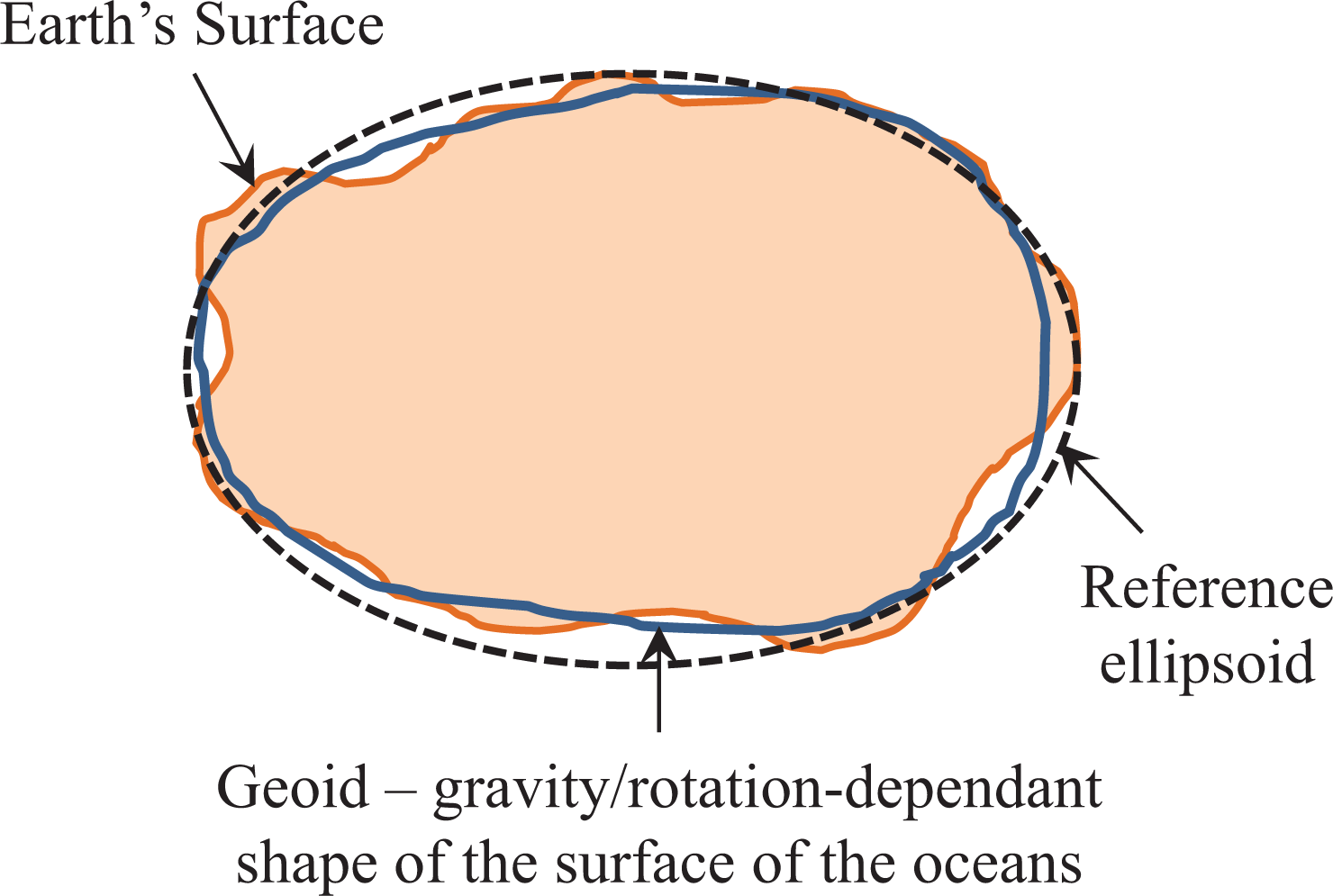
Ellipsoid approximation to the geoid.

The ellipsoid of revolution (sometimes called spheroid) has been used as the preferred surface on which point coordinates such as latitude (φ), longitude (λ), and elevation (h) are defined.^14,15

In this work, the surface of the ellipsoid of revolution is analyzed to enhance the mathematical model of the single FLP. This article is structured as follows. In “The ellipsoid and the spherical Earth” section, technical background on the ellipse and the ellipsoid are presented. Then, in “The FLP on ellipsoids” section, the integrated mathematical model of the Weber problem with ellipsoids is presented and discussed. The results of the ellipsoidal model are discussed in “Results” section. Finally, the conclusions and future work are presented in the last section.

The ellipsoid and the spherical Earth

An ellipse is defined as the set of all points P in a plane such that the sum of the distances of P from two fixed points (F and F′) in the plane is constant.¹⁶ Figure 3 presents an overview of the main elements that define an ellipse. Each of the fixed points is called a focus, and together they are called foci. The line segment V′ V through the foci is defined as the major axis, while the perpendicular bisector B′ B of the major axis is defined as the minor axis. Each end of the major axis (i.e. V and V′) is called a vertex. Finally, the midpoint of the line segment F′ F is called the center of the ellipse.¹⁶

Figure 3.

Ellipse with center at the origin.

An ellipsoid is the three-dimensional analogue of an ellipse. As presented in Figure 4, the ellipsoid consists of distinct semi-axis lengths a, b, and c. The Earth is approximated to an oblate ellipsoid where a = b > c.

Figure 4.

Triaxial ellipsoid with distinct semi-axis lengths.

The standard equation of an ellipsoid centered at the origin of a Cartesian coordinate system is expressed as follows:

\frac{x^{2}}{a^{2}} + \frac{y^{2}}{b^{2}} + \frac{z^{2}}{c^{2}} = 1.

Note that the ellipsoid may approximate to a sphere if a = b = c. By knowing this fact, coordinates in the ellipsoid can be expressed in terms of coordinates on the sphere. As presented in Figure 5, the position of a point P on the spherical model of the Earth’s surface is determined by the three main parameters: r (radial distance), θ (longitude), and φ (latitude).¹⁷

Figure 5.

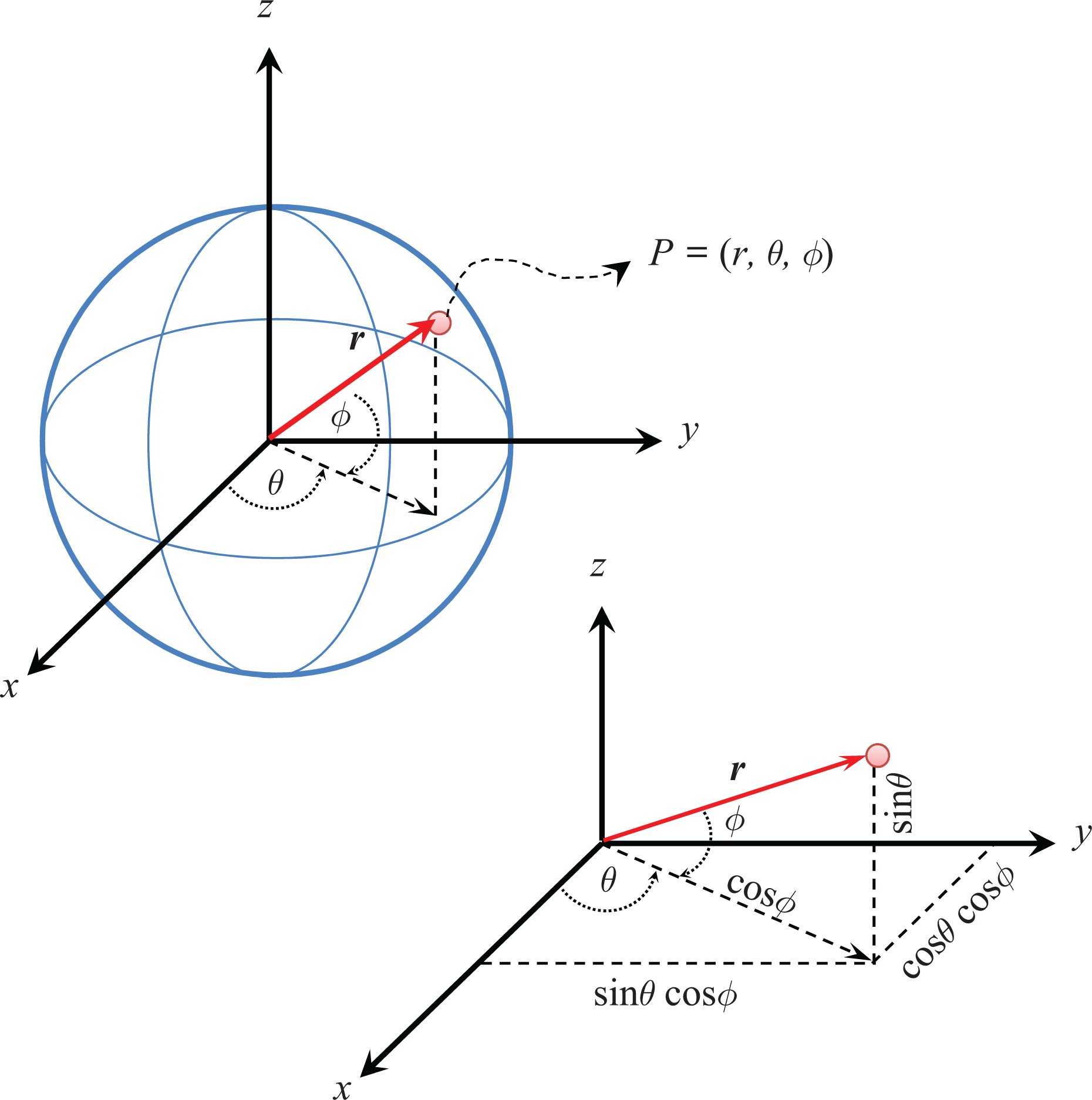
Spherical coordinate system.

With these parameters, the parametrization of a sphere of radius r centered at the origin can be expressed as follows^17
–19:

[\begin{matrix} x \\ y \\ z \end{matrix}] = [\begin{matrix} r cos φ cos θ \\ r cos φ sin θ \\ r sin φ \end{matrix}] .

The ellipsoid can be parametrized by slightly modifying the parametrization of the sphere¹⁹:

[\begin{matrix} x \\ y \\ z \end{matrix}] = [\begin{matrix} a cos φ cos θ \\ b cos φ sin θ \\ c sin φ \end{matrix}],

where $- \frac{π}{2} < φ \leq + \frac{π}{2}$ and −π < θ ≤ +π.

As presented in equation (3), the angles θ and φ do not represent geometric angles in the ellipsoid itself; these represent angles in the sphere with r = 1.

Distances on the sphere

The shape of the Earth’s surface is complex, and it is not comparable to any surface that can be modeled with simple mathematical formulation. Under the assumption that the shape of the Earth’s surface can be approximated to a sphere, any i-th point P_i on the surface can be defined by its latitude (φ_i) and longitude (θ_i).

The shortest distance or arc length between two points on the spherical surface is defined by:

(a) α_ij: the angle between the vectors that define the points P_i and P_j from the center of the sphere.^10,20 This angle is estimated as:

α_{i j} = Arccos [cos φ_{i} cos φ_{j} cos (θ_{i} - θ_{j}) + sin φ_{i} sin φ_{j}] .

(b) R: the radius of the sphere.

The arc length between two points P_i and P_j is expressed as:

l_{i j} = R \times α_{i j} .

The FLP on the sphere

Within the context of the single FLP on the sphere, there are r_i(φ_i, θ_i) demand points (clients), where i = 1, …, n, and r_j(φ_j, θ_j) potential locations on which it is possible to place a service point (facility). Each r_i(φ_i, θ_i) and r_j(φ_j, θ_j) points are connected by the arcs of length l_ij, which lie on the spherical surface. A weight w_i is associated to each demand point r_i(φ_i, θ_i). This weight may be associated to important data regarding the demand point such as the magnitude of the demand.²¹ Then, the single FLP consists of minimizing the weighted distances from the potential location of the facility to the customers.^8,10,21,22 The objective function is expressed as follows:

{min}_{φ, θ} f (r_{j}) = \sum_{i = 1}^{n} w_{i} l_{i j} .

The FLP on ellipsoids

Geodesics on the ellipsoid

A geodesic is defined as the shortest path between two points on a curved surface, particularly if the surface is treated as an ellipsoid of revolution.²³ When the Earth is considered as a sphere, the geodesics are great circles (all of which are closed). If the Earth is considered to be an oblate ellipsoid, the equator and the meridians are the only closed geodesics.²⁴ Figure 6 presents the geodesic AB on an ellipsoid of revolution where²³:

NA and NB are meridians;

s₁₂ is the length of the geodesic AB;

λ₁₂ is the longitude of B relative to A;

φ₁ and φ₂ are the latitudes of A and B, respectively;

α₀, α₁, and α₂ are the azimuths of the geodesic at E, A, and B, respectively.

Figure 6.

Geodesic AB on an ellipsoid of revolution where N is the north pole and E, H, and F lie on the equator.

From Figure 6, the arc delimited by the geodesic AB is identified. The geodesic of length s₁₂ connects two points: A at latitude and longitude (φ₁ and λ₁) and B at (φ₂ and λ₂). Within this context, two geodesic problems are usually considered²³:

Direct problem: It consists of finding the end point of a geodesic given its starting point (A), initial azimuth (α₁), and length (s₁₂). Thus, B and α₂ have to be determined.

Inverse problem: It consists of finding the shortest path between two given points. In this case, s₁₂, α₁, and α₂ have to be determined.

These problems involve solving the triangle NAB given an angle (α₁ for the direct problem and λ₁₂ = λ₁ − λ₂ for the inverse problem) and two adjacent sides.

For the purposes of the present work, the inverse problem is of particular interest. In the literature, there are methods to calculate the distance between two points on the ellipsoid’s surface as the shortest tangent method.²⁵ However, the direct and inverse iterative methods of Vincenty²⁶ are computationally efficient. Also, these methods are appropriate because the Earth’s surface is assumed to be an oblate spheroid, which is a closest approach to the true shape of the Earth. This assumption has led to the use of Vincenty’s methods for partitioning of the ellipsoidal Earth on regions for studies on meteorology, forestry, and biology.²⁷ In the “ Solution of the inverse problem” section, the basis of the method for the inverse problem of Vincenty²⁶ is reviewed to describe the adaptation performed for the present work.

Solution of the inverse problem

In “The ellipsoid and the spherical Earth” section, the parametrization of the ellipsoid from spherical coordinates was presented. Vincenty considered this information for the development of the inverse iterative method, and the following notation was defined as²⁶:

a and b: the major and minor semi-axes of the ellipsoid (a = 6378137 m according to WGS-84 and b = (1 − f)a where f = 1/298.2572221);

φ: the geodetic latitude, positive north of the equator;

f: the flattening of the spheroid = (a − b)/a;

U: the reduced latitude defined by tanU = (1 − f)tanφ;

λ: the difference in longitude on an auxiliary sphere;

σ: the angular distance between two points, P₁ and P₂, on the sphere;

S: the ellipsoidal distance between the points P₁ and P₂.

The pseudocode to estimate the length of s₁₂ (i.e. S) using the inverse method of Vincenty is presented in Figure 7.

Figure 7.

Pseudocode to estimate the length of the ellipsoidal distance between two points.²⁶

Integrated Weber model on ellipsoids

By considering the notation presented in “Solution of the inverse problem” section, the single FLP described by equation (6) can be adapted to the ellipsoid by defining the following terms:

$P_{f} (φ_{f}, λ_{f})$ : the coordinate (latitude and longitude) of the location of the service point;

$P_{i} (φ_{i}, λ_{i})$ : the coordinate (latitude and longitude) of the location of each i-th demand point (client) to be served by the facility (service point);

w_i: weight associated to each i-th demand point;

s_fi: ellipsoidal distance between the service point and the i-th demand point.

Then, the integrated Weber problem consists of finding the location of the facility $P_{f} (φ_{f}, λ_{f})$ that minimizes the total ellipsoidal distance to all clients. The objective function of the integrated Weber problem is expressed as follows:

mi n_{φ_{f}, λ_{f}} f = \sum_{i = 1}^{n} w_{i} s_{f i},

which is subject to:

\frac{{(a cos φ_{f} cos λ_{f})}^{2}}{a^{2}} + \frac{{(b cos φ_{f} sin λ_{f})}^{2}}{b^{2}} + \frac{{(c sin φ_{f})}^{2}}{c^{2}} = 1,

where $- \frac{π}{2} < φ_{f} \leq + \frac{π}{2}$ and $- π < λ_{f} \leq + π$ .

Results

Different sets of client points were considered to solve the FLP. For comparison purposes, the spherical model of the FLP was considered to analyze the feasibility of the FLP on ellipsoids. The results are discussed in the following sections.

Test set A: 10 randomly selected client points

For initial testing of the FLP model on ellipsoids, the client points presented in Table 1 were considered. The pseudocode presented in Figure 7 was implemented in Microsoft Excel 2010 for each client point. Then, the tool Solver Excel Solver from Frontline Solvers (R) was used to solve the objective function defined by equation (7) with the restrictions given by equation (8) considering all client points. For comparison purposes, the FLP was solved considering the assumption of the spherical Earth given by equation (6). For all client points, the weights were considered constant and equal to 1.0 (i.e. w_i = 1 for i = 1,…,10). Table 2 presents the optimal facility location points for the FLP on the ellipsoid and on the sphere. The value of the objective function represents the sum of all distances (in meters) from the facility to all client points. The location of each client point and the facilities (under spherical and ellipsoid models) are presented in Figure 8.

Table 1.

Latitude (ϕ) and longitude (λ) coordinates for the test set A.

Place	Coordinates
	Degrees		Radians
	Latitude	Longitude	Latitude	Longitude
Mexico City	19.391004	−99.283700	0.338437	−1.732827
Oklahoma, USA	35.482883	−97.759389	0.619293	−1.706223
Cusco, Peru	−13.497548	−71.558855	−0.235577	−1.248938
Algeria	27.753703	−7.355585	0.484394	−0.128379
Lusaka, Zambia	−15.416455	28.203666	−0.269068	0.492247
Belgium	50.497444	3.355396	0.881347	0.058563
Sidney, Australia	−33.796036	150.642244	−0.589852	2.629203
Hobart, Tasmania	−42.882375	147.319836	−0.748439	2.571216
Seoul, South Korea	37.565289	126.849465	0.655638	2.213941
Kabul, Afghanistan	34.553953	68.917539	0.603080	1.202838

Table 2.

Facility location for the test set A: location under the spherical and ellipsoidal models.

Earth model	Place	Latitude	Longitude	Objective function
Ellipsoid	Rumegies, France	50.497372	3.355883	85610240.31
Sphere	Rumegies, France	50.497513	3.355516	85679427.03

Figure 8.

As presented in Table 2, there is a difference of 69,186.72 m (approximately 69 km) between the total distances of the spherical and ellipsoid models. In Table 3, the individual distances from all client points to the located facility are presented. It can be observed that for some points, the distances are longer under the spherical model than for the ellipsoid model. However, for other client points, the distances are longer under the ellipsoid model. By considering the sum of all absolute differences, a total difference of approximately 142 km is estimated between the ellipsoid and the spherical distance models.

Table 3.

Facility location for the test set A: individual spherical and ellipsoidal distances.

Place	Coordinates (°)		Distance from facility to client point		Difference in distance: sphere model—ellipsoid model
Place	Latitude	Longitude	Ellipsoid model facility at (50.4973715° and 3.3558829°)	Sphere model facility at (50.4975134° and 3.3555155°)	Difference in distance: sphere model—ellipsoid model
Mexico City	19.391004	−99.283700	9212965.48	9209802.78	−3162.69
Oklahoma, USA	35.482883	−97.759389	7754251.16	7742875.01	−11376.16
Cusco, Peru	−13.497548	−71.558855	10106467.76	10129302.96	22835.20
Algeria	27.753703	−7.355585	2682447.74	2686024.19	3576.45
Lusaka, Zambia	−15.416455	28.203666	7693013.34	7720352.11	27338.78
Belgium	50.497444	3.355396	35.43	11.49	−23.94
Sidney, Australia	−33.796036	150.642244	16758291.99	16781877.56	23585.57
Hobart, Tasmania	−42.882375	147.319836	17142494.16	17170824.66	28330.50
Seoul, South Korea	37.565289	126.849465	8792623.10	8775612.79	−17010.30
Kabul, Afghanistan	34.553953	68.917539	5467650.15	5462743.47	−4906.69
	Total distance		85610240.31	85679427.03	69186.72
				Absolute difference	142146.28

The distance differences presented in Table 3 must be considered during budget and delivery time planning due to the significance of some of them (i.e. 22.835 km for Cusco, Peru, 27.338 km for Lusaka, Zambia, and 28.330 km for Hobart, Tasmania). Because most of the distance differences are positive (considering the spherical model as reference), it can be assumed that distances on the spherical model are longer than the distances on the ellipsoid model. However, this assumption changes for specific regions.

Due to this finding, budget and delivery planning for the FLP should consider the ellipsoid model because the spherical model does not consider changes in the Earth’s surface across all regions. The ellipsoid model considers these changes for each Earth’s quadrant. The information presented in Table 3 corroborates this finding.

Test set B: Three client points on the Western Hemisphere and seven on the Eastern Hemisphere

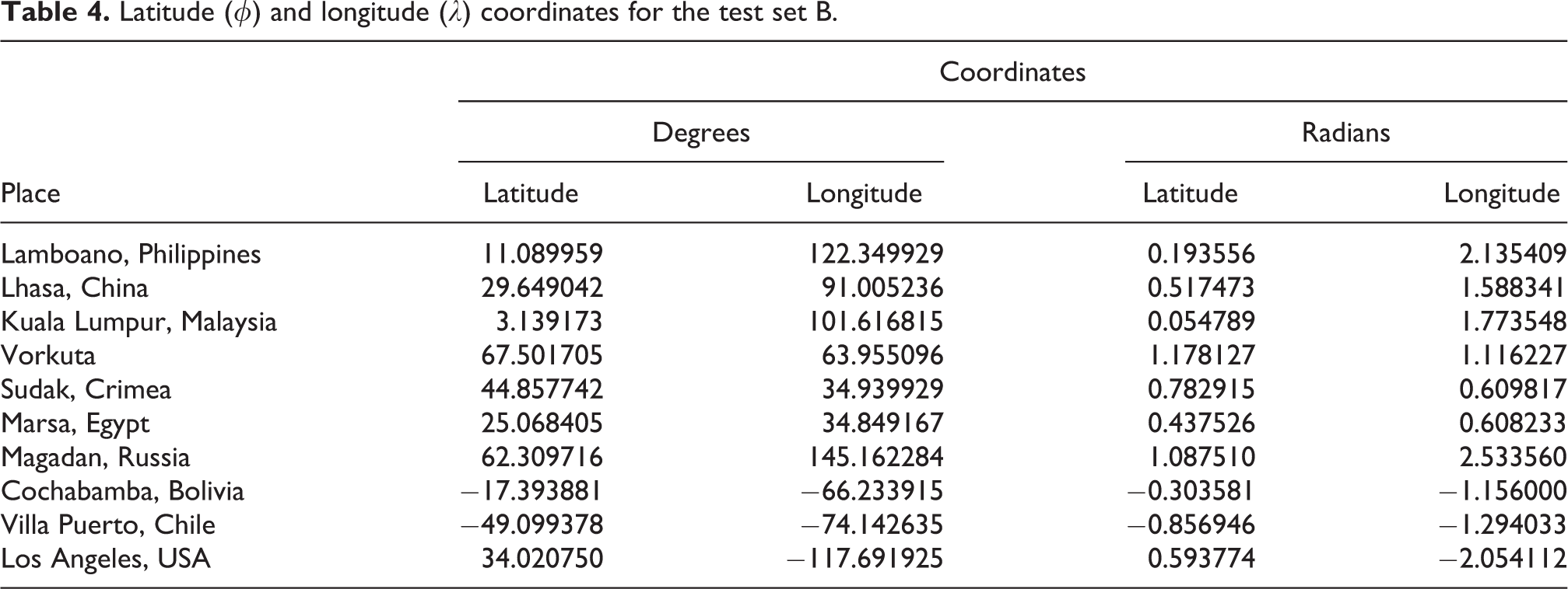
The second testing considered the robustness of the FLP under the spherical and ellipsoid models for changes in the density of client points. For this case, the points presented in Table 4 were considered. Table 5 presents the optimal facility location points for the FLP on the ellipsoid and on the sphere for these points. Then, the location of each client point and the facilities (under spherical and ellipsoid models) are presented in Figure 9.

Table 4.

Latitude (φ) and longitude (λ) coordinates for the test set B.

Place	Coordinates
	Degrees		Radians
	Latitude	Longitude	Latitude	Longitude
Lamboano, Philippines	11.089959	122.349929	0.193556	2.135409
Lhasa, China	29.649042	91.005236	0.517473	1.588341
Kuala Lumpur, Malaysia	3.139173	101.616815	0.054789	1.773548
Vorkuta	67.501705	63.955096	1.178127	1.116227
Sudak, Crimea	44.857742	34.939929	0.782915	0.609817
Marsa, Egypt	25.068405	34.849167	0.437526	0.608233
Magadan, Russia	62.309716	145.162284	1.087510	2.533560
Cochabamba, Bolivia	−17.393881	−66.233915	−0.303581	−1.156000
Villa Puerto, Chile	−49.099378	−74.142635	−0.856946	−1.294033
Los Angeles, USA	34.020750	−117.691925	0.593774	−2.054112

Table 5.

Facility location for the test set B: location under the spherical and ellipsoidal models.

Earth model	Place	Latitude	Longitude	Objective function
Ellipsoid	—	62.340203	61.282898	70,636,370.66
Sphere	—	63.081217	61.762400	70,654,088.90

Figure 9.

According to the results presented in Table 5 and Figure 9, it can be observed that the facility is to be located within the region where most of the client points are located. This is observed for the FLP under the spherical and ellipsoid models. As presented in Table 5, there is a difference of approximately 17.71 km between the total distance of the ellipsoid model and the spherical model. These results are consistent with those presented in Table 2.

Test set C: Seven client points on the Western Hemisphere and three on the Eastern Hemisphere

The final testing considered an inverse balance on the density of client points presented in “Test set B: Three client points on the Western Hemisphere and seven on the Eastern Hemisphere” section. As presented in Figure 10, the facility (under the spherical and ellipsoid models) is located within the region where most of the client points are located (in this case, in the Western Hemisphere). In Table 6, the location for these facilities is presented where a difference of approximately 43.34 km exists between the total distances of both models.

Figure 10.

Table 6.

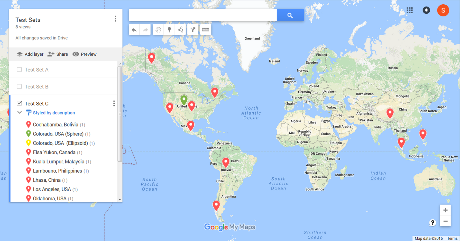
Facility location for the test set C: location under the spherical and ellipsoidal models.

Earth model	Place	Latitude	Longitude	Objective function
Ellipsoid	Colorado, USA	40.005242	−104.782944	67,108,510.34
Sphere	Colorado, USA	40.036900	−104.694222	67,151,851.88

Conclusions and future work

Based on the results presented in “Test set A: 10 randomly selected client points”, “Test set B: Three client points on the Western Hemisphere and seven on the Eastern Hemisphere, and “Test set C: Seven client points on the Western Hemisphere and three on the Eastern Hemisphere” sections, minimum total coverage distance is achieved with the FLP considering the ellipsoid as the model for the Earth’s surface. This distance is smaller than the total coverage distance achieved under the spherical model.

However, depending on the location of the client points across the hemispheres, the magnitude of this difference may increase or decrease. This is because the ellipsoid model considers quadrant-dependent changes in the Earth’s surface. This is an assumption closer to the real surface changes of the Earth which are not considered by the spherical model. Hence, more accurate facility location results can be obtained with the ellipsoid logistic model presented in this work.

These quadrant-dependent distance changes must be considered by the enterprise because budget planning related to factors such as lead times, transportation costs, CO₂ emissions, and so on is dependent on the estimated travel distances from the facility to the client points.^28,29 Thus, current cost optimization approaches to strategic logistic costs should incorporate the ellipsoid model for the FLP and routing plans.

Finally, the FLP on the ellipsoid has the same behavior than the FLP on the sphere or on the plain regarding the location of the facility when most of the client points are concentrated within a specific region. In this case, the facility will be located within the region where most of the clients are located. This observation is important to preliminarily estimate the jurisdiction of the facility.

The present work can be extended into the following points regarding the FLP and vehicle routing problem fields:

integrate the ellipsoid model within the capacitated FLP³⁰ and the multifacility location problem³¹ to analyze the effect on deterministic and stochastic demand coverage and

consider alternative surfaces for the FLP (i.e. toroidal, Riemannian,³ or quasigeoidal¹²).

Footnotes

Declaration of Conflicting Interests

The author(s) declared no potential conflicts of interest with respect to the research, authorship, and/or publication of this article.

Funding

The author(s) disclosed receipt of the following financial support for the research, authorship and/or publication of this article: Our institution, Universidad Popular Autonoma del Estado de Puebla, provided the funding for the Article Processing Charge (APC) of 600USD.

References

Lambiase

Mastrocinque

Miranda

. Strategic planning and design of supply chains: a literature review. Int J Eng Bus Manag 2013; 5(49): 1–11.

Carro

González

. Administración de las operaciones: actividades para el aprendizaje. 1st ed. Mar del Plata: Universidad Nacional de Mar del Plata, Facultad de Ciencias Económicas y Sociales, 2015.

Tokgöz

Alwazzi

Trafalis

. A heuristic algorithm to solve the single-facility location routing problem on Riemannian surfaces. Comp Manag Sci 2015; 12(3): 397–415.

Shih

. Facility location decisions based on driving distances on spherical surface. Am J Oper Res 2015; 5: 450–492.

Reid

Sanders

NR.

Operations management. 5th ed. Hoboken, New Jersey: John Wiley & Sons, 2013.

ReVelle

Eiselt

. Location analysis: a synthesis and survey. Eur J Oper Res 2005; 165(1): 1–19.

Katz

Cooper

. Optimal location on a sphere. Comput Math Appl 1980; 6(2): 175–196.

Drezner

. A solution to the Weber location problem on the sphere. J Oper Res Soc 1985; 36: 333–334.

Aykin

Babu

. Multifacility location problems on a sphere. Int J Math Math Sci 1987; 10(3): 583–596.

10.

Nava

. El problema de la mejor ubicación de un centro de servicio sobre una esfera. Puebla: Benemérita Universidad Autónoma de Puebla, Facultad de Ciencias Fisico Matemáticas, 2011.

11.

National Aeronautics and Space Administration (NASA). Gravity recovery and climate experiment (GRACE): gravity anomaly maps and the geoid. http://earthobservatory.nasa.gov/Features/GRACE/page3.php (accessed 12 December 2015).

12.

Mysen

. GOCE quasigeoid performance for Norway. Int J Appl Earth Obs Geoinf 2015; 35(Part A): 136–139.

13.

Fraczek

. Mean sea level, GPS, and the geoid. Esri Applications Prototype Lab, http://www.esri.com/news/arcuser/0703/geoid1of3.html (accessed On 12 December 2015).

14.

Avalos

. El geoide para el área mexicana y sus aplicaciones. Notas: Revista de Información y Análisis 2002; 20: 25–30.

15.

Janssen

. Understanding coordinate systems, datums, and transformations in Australia. In: Ostendorf

Baldock

Bruce

Burdett

Corcoran

(eds) Proceedings of the Surveying & Spatial Sciences Institute Biennial International Conference, Adelaide, Australia, 28 September–2 October 2009, pp. 697–715. Surveying & Spatial Sciences Institute.

16.

Barnett

Ziegler

Byleen

College algebra: a graphing approach. New York: McGraw Hill Higher Education, 2000.

17.

Surowski

. Distance between points on the earth’s surface. In: Department of Mathematics: Kansas State University, 2011, pp. 1–4. https://www.math.ksu.edu/~dbski/writings/haversine.pdf.

18.

Karttunen

Kröger

Oja

Poutanen

Donner

(eds). Fundamental Astronomy, Chapter 2: Spherical Astronomy. 5th ed. New York: Springer Berlin Heidelberg, 2007, pp. 11–46.

19.

Joyce

. Gallery of surfaces: math 131 multivariate calculus. In: Department of Mathematics and Computer Science: Clark University, 2014, pp. 1–11. http://aleph0.clarku.edu/~djoyce/ma131/gallery.pdf~dbski/writings/haversine.pdf

20.

Dhar

Rao

. Domain approximation method for solving multifacility location problems on a sphere. J Oper Res Soc 1982; 33(7): 639–645.

21.

Fernandes

Aloise

. On the Weber facility location problem with limited distances and side constraints. Optim Lett 2014; 8(2): 407–424.

22.

Stanimirović

Ćirić

. Discrete location problem on arbitrary surface in R ³*. FACTA UNIVERSITATIS, Ser Math Inf 2010; 25: 47–56.

23.

Karney

. Algorithms for geodesics. J Geodesy 2013; 87(1): 43–55.

24.

Wikipedia. Geodesics on an ellipsoid. https://en.wikipedia.org/wiki/Geodesics_on_an_ellipsoid (accessed 12 December 2015).

25.

Zhang

Zhao

Yang

. Ellipsoid earth path planning based on shortest tangent method. In Jeng-Shyang

Pan

Xueying

Zhang

Chin-Shiuh

Shieh

Wendong

Zhang

(eds) Proceedings of the 2012 international conference on computing, measurement, control and sensor networks, Taiyuan, Shanxi, China, 7–9 July 2012, pp. 298–301. Los Alamitos, CA: IEEE Computer Society, Conference Publishing Services (CPS).

26.

Vincenty

. Direct and inverse solutions of geodesics on the ellipsoid with application of nested equations. Surv Rev 1975; XXII(176): 88–93.

27.

Liu

. Voronoi diagram generation on the ellipsoidal earth. Comput Geosci 2014; 73: 81–87.

28.

Melo

Nickel

Saldanha-da-Gama

. Facility location and supply chain management—a review. Eur J Oper Res 2009; 196: 401–412.

29.

Elhedhli

Merrick

. Green supply chain network design to reduce carbon emissions. Transport Res D Tr E 2012; 17(5): 370–379.

30.

Fasano

JP,

Tan

. Location problems for supply chain. In: Renko

(ed.) Supply chain management—new perspectives . Rijeka: InTech, 2011, pp. 321–336.

31.

Iyigun

Israel

. A generalized Weiszfeld method for the multi-facility location problem. Oper Res Lett 2010; 38(3): 207–214.

Logistic model for the facility location problem on ellipsoids

Abstract

Keywords

Introduction

The ellipsoid and the spherical Earth

Distances on the sphere

The FLP on the sphere

The FLP on ellipsoids

Geodesics on the ellipsoid

Solution of the inverse problem

Integrated Weber model on ellipsoids

Results

Test set A: 10 randomly selected client points

Test set B: Three client points on the Western Hemisphere and seven on the Eastern Hemisphere

Test set C: Seven client points on the Western Hemisphere and three on the Eastern Hemisphere

Conclusions and future work

Footnotes

Declaration of Conflicting Interests

Funding

References