Sage Journals: Discover world-class research

Abstract

Moderation is a commonly used technique in psychological studies to investigate how the relationship between two variables is affected by a third variable, the moderator. The findings have practical implications because they inform practitioners when a relationship is strong or weak, or how to reduce the adverse impact of a factor or enhance the positive impact of a factor. However, insufficient details have been reported in some cases, making it difficult for readers to interpret the results. For example, the meaning of the term main effect may not be clear; the full sample standard deviation may be used unconditionally for the plotting of simple effects; the meaning of the coefficient of the product term in the standardized solution may be unclear; and the formation of the standard errors and confidence intervals in the standardized solution might be biased. As a snapshot of the common practices in psychology, a systematic review of moderation studies on a selected topic—autism—was conducted to illustrate the prevalence of some of these issues. Numerical examples illustrate the problems with common practices, and recommendations are presented to help applied researchers improve their moderation analysis practices, ensuring that their values are interpretable.

Keywords

moderation regression standardization

Moderation is a frequently studied phenomenon in psychology. In its simplest form, moderation is present when the effect of one variable on another variable depends on the level of a third variable. For example, the effect of treatment conditions on post-treatment anxiety increases as social cognition increases (Hollocks et al., 2023). Alternatively, the effect of treatment is strong in one population but weak, zero, or even reversed in sign in another population. Moderation has several theoretical and practical implications (Lash et al., 2021). First, intellectually, it helps us understand more about the stability of the effect of one variable on another, such as whether its effect is stronger in one condition but weaker or even zero in another condition. Second, it helps us understand when an intervention is useful, when it is less useful, or even when it is useless, and to allocate resources accordingly. Third, it helps us find ways to improve the effect of an intervention or reduce the adverse impact of a risk factor.

In addition to moderation, standardization is a common technique in psychology when doing analysis and reporting the results. In psychology, many variables are measured in arbitrary units, such as means on a Likert scale or just scores assigned to options. To make the results more interpretable, it is common to standardize the variables of concern, using the mean as the center of the distribution and the standard deviation (SD) as the unit of measurement. Therefore, instead of saying that a person has a score of 3 on parental burnout, we can say that this person is 1.5 SD above the mean (e.g., Liu et al., 2024). When talking about the effect of a variable, instead of saying that an increase of one unit of parenting stress leads to an increase of three units of the predicted value of parental burnout, we say that an increase of 1 SD of parenting stress, such as a change from the mean to 1 SD above the mean (or, equivalently, a change from 1 SD below the mean to the mean), leads to an increase of 0.5 SD of the predicted value of parental burnout (e.g., Liu et al., 2024).

Despite the popularity of moderation in psychological studies, we have observed several incorrect or imperfect practices, including practices related to moderation without standardization and practices related to moderation with standardization. In this article, we briefly describe the moderation model in multiple regression. We then present a systematic review of the common practices in moderation analysis in a selected area of clinical psychology. Lastly, we present the problems with some common practices and our recommendations on how to carry out analysis and report the results.

A Brief Description of Moderation Conducted by Multiple Regression

We use a multiple regression model estimated by ordinary least squares (OLS) for this brief description, although some of the problems discussed later can be generalized to moderation analysis conducted in other frameworks, such as structural equation modeling and multilevel modeling. Suppose we are going to investigate whether the effect of a predictor, X, called the focal variable below, on an outcome variable, Y, is moderated by (depends on) the level of W, the moderator. This is the regression model:
$Y = B_{0} + B_{X} X + B_{W} W + B_{X W} X W + e$

We call this the unstandardized model, which does not involve rescaling any variables by sample standard deviations, to differentiate it from the standardized solution below, and from the practice of doing standardization before doing the regression analysis, for reasons to be explained later. In the model, XW is the product of X and W, and e is the error term. We have not included control variables because they will only affect the intercept (Β₀) and will not affect the phenomena to be discussed. Although sometimes misinterpreted (discussed later), conventionally, the coefficients of the components, Β _X and Β _W , are called the main-effect terms or simply main effects of X and W, respectively.

This model can be rearranged as follows:
$Y = (B_{0} + B_{W} W) + (B_{X} + B_{X W} W) X + e$

It is then apparent that the model is equivalent to saying that the effect of X is a linear function of W, Β _X + Β_XWW. The coefficient of the product term, Β _XW , is the moderation effect. This model also shows that the coefficient of X, Β _X , is a conditional effect (also called a simple effect) of X: the effect of X when W = 0. The moderation effect can be tested by testing the null hypothesis that Β _XW = 0. If the moderation effect is significant, it can be examined by calculating the conditional effect. Suppose W is a dichotomous variable represented by a dummy variable (coded 0 for one group and 1 for the other group). In this case, there are only two conditional effects, when W = 0 and when W = 1:
$W = 0 : Y = B_{0} + B_{X} X + e$

$W = 1 : Y = (B_{0} + B_{W}) + (B_{X} + B_{X W}) X + e$
If W is continuous, usually two or three levels are selected—for example, high, medium, and low levels of W are defined as 1 SD below the mean, the mean, and 1 SD above the mean:
$\begin{aligned} W is High (W_{High} & = M_{W} + S D_{W}) : Y = (B_{0} + B_{W} W_{High}) \\ + (B_{X} + B_{X W} W_{High}) X + e \end{aligned}$

$\begin{aligned} W is Medium (W_{Medium} & = M_{W}) : Y = (B_{0} + B_{W} W_{Medium}) \\ + (B_{X} + B_{X W} W_{Medium}) X + e \end{aligned}$

$\begin{aligned} W is Low (W_{Low} & = M_{W} - S D_{W}) : Y = (B_{0} + B_{W} W_{Low}) \\ + (B_{X} + B_{X W} W_{Low}) X + e \end{aligned}$
Instead of, or in addition to, reporting three conditional effects, it is common to visualize the conditional effects using a plot of Y against X, with two or three lines corresponding to the conditional effects.

Although not a must (Hayes, 2022) and it has been sometimes conducted due to the misconception that it is “necessary” to remove or reduce multicollinearity between the product term and its components (for a discussion of this “myth,” see Hayes, 2022, pp. 320–328), mean-centering is sometimes used when testing a moderation effect. Let M_X and M_W be the means of X and W, respectively, and X _c be X − M_X and W_c be W − M_W. The mean-centered regression model is:
$Y = B_{0}^{''} + B_{X_{C}}^{''} X_{C} + B_{W_{C}}^{''} W_{C} + B_{X_{C} W_{C}}^{''} X_{C} W_{C} + e$

$Y = (B_{0}^{''} + B_{W}^{''} W_{C}) + (B_{X}^{''} + B_{X_{C} W_{C}}^{''} W_{C}) X_{C} + e$

The coefficient of the product term, $B_{X_{C} W_{C}}^{''}$ , is identical to Β _XW , while the coefficients $B_{X_{C}}^{''}$ and $B_{W_{C}}^{''}$ can be different from Β _X and Β _W . However, as demonstrated by Hayes (2022), the conditional effect for a level of W_c computed from this model, including its standard error and p-value, will be identical to that computed from the model without mean-centering for the corresponding level of W. For example, when W is equal to its mean, the effect of X is Β _X + Β_XWM_W from the original model, which is equal to the coefficient $B_{X_{C}}^{''}$ , the effect of X_c when W_c = W – M_W = 0. Other than making the coefficient of X and W easier to interpret, however, mean-centering offers no advantage over hypothesis testing and the estimation of the conditional effects and moderation effects.

If standardization is necessary to make the coefficients more interpretable, as is usually done in multiple regression, Friedrich (1982; see also Aiken & West, 1991) shows that standardization needs to be done before forming the product term. For example, if Y, X, and W are to be standardized, denoted by Z_Y, Z_X, and Z_W, respectively, this is the model:
$Z_{Y} = B_{0}^{'} + B_{X}^{'} Z_{X} + B_{W}^{'} Z_{W} + B_{X W}^{'} Z_{X} Z_{W} + e$

If W is a dichotomous variable and so should not be standardized (Darlington & Hayes, 2016), this is the model:
$Z_{Y} = B_{0}^{'} + B_{X}^{'} Z_{X} + B_{W}^{'} W + B_{X W}^{'} Z_{X} W + e$

We refer to these models, with at least one variable standardized, as the standardized model. Note that if confidence intervals (CIs) are to be presented for coefficients with the variables standardized, as shown by Yuan and Chan (2011), the standard errors obtained by doing standardization before doing OLS regression are biased. Analytical solutions have not yet been developed for models with a moderator, and Cheung et al. (2022) argue that bootstrapping is a viable option.

A Systematic Review of Moderation Analysis in Studies on Autism Spectrum Disorder

Given the huge popularity of moderation analysis in psychology, it is impossible to do a review of the practice of moderation analysis in all areas of psychology. To shed light on the current practice in moderation analysis, we selected an applied area in which moderation analysis is popular—the study of autism spectrum disorder (ASD) in clinical psychology. We conducted a systematic review of studies that involve moderation analysis.¹ This area was selected due to the resources available at the time of conducting the review. Moreover, this area is an applied one, and the literature on moderation cited in the articles reviewed is also typically cited in other areas of psychology. Therefore, although we selected this topic for the systematic review, we believe the findings can give insights into how moderation needs to be done in other areas of psychology.

Online electronic searches were conducted in December 2023 in three databases: APA PsycINFO, ERIC, and MEDLINE. During the initial literature search, we applied the keywords moderate, moderator, moderation, and moderating along with the search terms ASD, autism, and autism spectrum disorders to screen for articles that used moderation analysis relating to ASD. To ensure that we captured the current state of moderation practices in ASD studies, we limited our search to articles published between 2020 and 2023.

The electronic search returned 1,979 articles. Duplicates were identified and removed, leaving 1,638 articles to be screened. The second author rated the titles and abstracts to assess for evidence of some form of moderation analysis having been conducted. Both authors then screened 451 full-text articles for eligibility under the following inclusion criteria: (1) reporting of the path coefficients and (2) the use of regression-like methods (e.g., multiple regression, structural equation modeling, logistic regression, and path analysis). Articles were excluded if (1) no moderation effect was tested; (2) there was no data collection; or (3) they were meta-analyses and/or systematic reviews. Articles were also excluded if they did not use regression-like methods, did not provide enough information, were not written in English, had restricted access, or were not focused on ASD or ASD participants. The full systematic review strategy is detailed in the Preferred Reporting Items for Systematic reviews and Meta-Analyses (PRISMA) flow diagram shown in Figure 1.

Figure 1.
PRISMA Flow Diagram.

Among the final 146 articles used for the systematic review, 61.0% examined numerical moderators, 28.1% examined categorical moderators, and 11.0% employed both numerical and categorical moderating variables. When reporting the moderation results, around two-thirds of the studies reported the unstandardized coefficients, usually denoted by B (66.4%), while 25.1% of the studies did not. Almost half of the articles reported either the standard errors or 95% CIs (47.3%), while 26.0% reported both. Around a quarter of the studies did not report standard errors or CIs (26.7%). Lastly, 45.9% of the studies included the term main effect, usually referring to the coefficient of the focal variable (or moderator) in the model with the product term.

For most of the articles, only the final models with the moderation product term were reported (89.3%). In comparison, 7.1% of the studies’ models also reported the model that did not include the product term. In some cases, it was unclear whether the product term was included in a reported model (3.6%). A substantial number of the articles reported at least one non-significant product term (78.6%). There was one article that presented a special case where product terms were significant but became non-significant after “deleting cases with undue influence” (Yoder et al., 2021, p. 63). Finally, 58.9% of the studies included at least one plot of simple effects (with an additional 1.4% needing to be accessed through supplementary tables). In comparison, the remaining 39.7% did not provide plots of simple effects.

Of the articles reviewed, 30.8% reported that mean-centering was conducted, and 40.4% reported that mean-centering and/or standardization was conducted before fitting a model. Note that if a variable was standardized, it was also mean-centered (had a mean of zero). Despite the popularity of mean-centering in the literature, we could not assume that mean-centering was also conducted for the remaining studies. For example, one popular tool for moderation analysis, the PROCESS macro (Hayes, 2022), does not do mean-centering by default. Users need to add an argument (center = 1) to request mean-centering explicitly (Hayes, 2022, p. 328). Therefore, even when this tool was used in an article, we could not assume that mean-centering was conducted unless the authors explicitly reported that this was so.

It was also found that 45.9% of the articles reported the standardized beta coefficient, usually denoted by β, while an equal percentage of the articles did not report the standardized beta coefficient. For the articles reporting the standardized beta coefficient, only 12.5% stated that standardization was conducted before the product term was formed (as proposed by Friedrich, 1982). It is not clear how standardization was conducted for the product term for the remaining 87.5% of the articles. When standardized coefficients were requested, some programs reported the coefficients with all terms standardized, including the product term. Therefore, we could not ascertain what the coefficient of the product term referred to, even though it is possible that standardization was conducted correctly for these articles.

In sum, most of the studies conducted moderation appropriately; the standardized results were commonly reported; and plots of simple effects were usually used to investigate the pattern of a moderation effect. However, when interpreting the unstandardized coefficients of the focal variable for which the effect was moderated (the so-called main effect), it is sometimes difficult to determine how the coefficients should be interpreted because it is not clear whether mean-centering was conducted. When standardization results are reported, it is also not unusual for insufficient information to be provided to (a) evaluate whether the standardization was conducted correctly, making it difficult to interpret the coefficient of the product term, and (b) whether the standard errors and CIs were formed correctly for the standardized solution. We will focus on these issues in the following sections.

Doing and Reporting Moderation Right (and How To Do It Wrong)

In this section, we discuss some issues regarding conducting and reporting moderation effect analysis. The code for the numerical examples can be downloaded from the Open Science Framework project for this article.² The publicly available data set autism_data_large from the R package mgm (Haslbeck & Waldorp, 2020) is used for illustration. It is a large data set with data collected by the Dutch Association for Autism from 3,521 Dutch participants. For illustration, we only retained cases aged 18 or above, with a total of 2,029 participants (for a detailed description of the data set, see Deserno et al., 2017). All of the plots were generated using the plot() function from the manymome package developed by Cheung and Cheung (2024). The stdmod package, developed by Cheung et al. (2022), was also used to demonstrate appropriate standardization and CIs for the standardized coefficients. All illustrations were conducted in the R environment (R Core Team, 2024). Although basic knowledge of R is required to replicate the results, it is not required to understand the phenomena discussed here.

We need to stress that the models fitted below are atheoretical, and control variables are not included to keep the models simple. The variables have been selected solely to illustrate the problems with some practices. Although not intended to reveal any findings of theoretical importance, these models are sufficient to illustrate the problems and shed light on how other studies of theoretically important models should be conducted.

Unstandardized Solution

When standardization was not carried out, most studies conducted moderation and reported the results correctly, partly because the steps are simple and there are user-friendly tools for moderation analysis—for example, Hayes’ (2022) PROCESS macro. However, we still found two aspects where the reporting and interpretation of results without standardization could be improved.

Interpreting the So-Called Main Effect (Especially When the Product Term Is Not Significant)

We observed that some studies only reported the results of models with product terms included, even when the moderation effect was not significant, leading the authors to interpret the results as indicating the absence of moderation. The coefficient of the focal variable in these moderated regression models is then interpreted. It is correct that, in testing the moderation effect, it is unnecessary to test a model without the product term (Hayes, 2022). However, even if the product term is not significant, unless the sample estimate of the coefficient of this product term is exactly zero, the coefficient of the focal variable is still a conditional effect (when the moderator is zero) and so will depend on the scaling of the moderator. Hayes (2022) writes:
it is neither appropriate to interpret b₁ [the coefficient of X] as relationship between X and Y controlling for W “on average” or “controlling for W and XW,” nor is it the “main effect of X” (to use a term from ANOVA [analysis of variance] lingo). (p. 243)

We do not oppose using main effect as a label or name for the coefficient of X. This term was used frequently (about 45%) in the articles included in this systematic review. However, as pointed out by an anonymous reviewer, sometimes researchers use the term main effect in moderated regression in the same way as it is used in ANOVA. Therefore, we first discuss the meaning of the main effect in ANOVA and then the case in moderated regression with X and/or W continuous.

When Both X and W Are Dichotomous

First, we consider the case when both X and W are dichotomous (X1 versus X2 and W1 versus W2). Hayes (2022) demonstrates how, in this case, a moderated regression model is equivalent to a two-by-two between-subject ANOVA (pp. 308–315). First, he shows two interpretations of the main effect in this ANOVA model. Suppose we denote the means in the group X1W1, X1W2, X2W1, and X2W2 by M₁₁, M₁₂, M₂₁, and M₂₂, respectively. The marginal means of X are then M₁ = (M₁₁ + M₁₂) / 2 and M₂ = (M₂₁ + M₂₂) / 2 for X1 and X2, respectively. One interpretation of the main effect of X is the difference in the marginal means of X: M₂ – M₁. Another interpretation is the (unweighted) average of the conditional effects of X in the two levels (groups) of W: [(M₂₁ – M₁₁) + (M₂₂ – M₁₂)] / 2. These two values are identical. They are just different meanings of the main effect.

Suppose this is what researchers mean by the main effect in moderated regression with dichotomous X and W. In this case, we certainly can use the term main effect, given that the moderated regression model and the two-by-two ANOVA model are equivalent. However, there is one caveat. If we fit a moderated regression model in this case to have the coefficients of X and W correspond to the main effects as in ANOVA, Hayes (2022) demonstrates that a coding scheme such as −0.5 versus 0.5 is needed—termed the “main effect parameterization” (p. 313). When coded in this way, the coefficient of X, which is the effect of X when W = 0, is the main effect in the two-by-two ANOVA model. However, in this coding scheme, W = 0 represents neither group. No case can have W = 0, not even in the population, if W represents a genuine categorical variable (e.g., City A versus City B).

However, when the moderation effect is fitted by regression, dummy coding is usually used, with 0 for one group and 1 for the other.³ With this coding scheme, termed “simple effect parameterization” by Hayes (2022, p. 313), the coefficient of X is not the main effect as in a two-by-two ANOVA. Instead, it is the effect of X in one of the groups of W, either (M₂₁ – M₁₁) or (M₂₂ – M₁₂), as defined above.

Therefore, even in the special case of dichotomous X and W, which is equivalent to the two-by-two ANOVA model, researchers need to specifically code X and W to be able to interpret their coefficients as the main effects, as in ANOVA. Otherwise, it is misleading to call them the main effects when they are conditional effects.

When X is Numerical and W is Dichotomous

If W is dichotomous (W1 versus W2) and represented by a dummy variable, then the coefficient of X in the moderated regression model is the effect of X in the group W = 0. Suppose we use satisfaction with work again as the focal variable and use gender as a moderator. The estimates with gender coded as male = 0 and female = 1 are shown in Table 1.

Table 1.
Moderated Regression—Unstandardized—Categorical Moderator (Male = 0, Female = 1).

B SE t p

Constant 1.329 0.325 4.093 <.001*

sat_work 1.357 0.095 14.249 <.001*

gender −0.509 0.613 −0.830 .406

sat_work × gender 0.073 0.181 0.405 .686

Note: p < .001.

The product term is not significant, and the coefficient of satisfaction with work is 1.357.

The estimates with gender coded as female = 0 and male = 1 are shown in Table 2.

Table 2.
Moderated Regression—Unstandardized—Categorical Moderator (Female = 0, Male = 1).

B SE t p

Constant 0.820 0.520 1.576 .115

sat_work 1.430 0.154 9.313 <.001

gender −0.509 0.613 −0.830 .406

sat_work × gender −0.073 0.181 0.405 .686

Note: ***p < .001.

The coefficient of satisfaction with work is 1.430, different from that with male = 0. Therefore, the coefficient of X (satisfaction with work) depends on the coding scheme of the moderator, even though the moderation effect is not significant. We also cannot call the coefficient of X as “the” main effect because it depends on the coding scheme.

If we want to define main effect in this case as in 2-by-2 ANOVA, we may define it as the (unweighted) average of the effects of X in the two groups. As in the previous case, instead of using dummy coding, we need to use a coding scheme such as –0.5 and 0.5 for W. For example, if we want to make the coefficient of X (satisfaction with work) interpretable as the main effect defined above, we can code female = –0.5 and male = 0.5 (or vice versa).

As shown in Table 3, the coefficient of X is 1.393. This is the mean of the effects of X in the male group (1.430) and the female group (1.357) (up to rounding error). Therefore, as in the case when both X and W are dichotomous, to interpret the coefficient of X as the main effect as defined above is possible, but we need a special coding scheme, which is rarely the case in applied research, and so it is wrong to call the coefficient as the main effect if we want to use this term more than just a label. However, even when a moderator was dichotomous, the coefficient of the focal variable was sometimes still interpreted as the main effect (e.g., Tabak et al., 2020, p. 5 and Table 2) without making it clear what this effect refers to: the effect of the focal variable in one group (and then it is certainly not a main effect), or the average conditional effect (which requires a special coding scheme for the dichotomous moderator).

Table 3.
Moderated Regression—Unstandardized—Main Effect Coding (Female = –0.5, Male = 0.5).

B SE t p

Constant 1.074 0.307 3.504 <.001*

sat_work 1.393 0.090 15.425 <.001*

Gender 0.509 0.613 0.830 .406

sat_work × gender −0.073 0.181 −0.405 .686

When Both X and W are Numerical

If W is also a numeric variable, then the dependence of the coefficient of X on the coding is more apparent.

Suppose we transform a moderator using a linear transformation: $W^{'} = (W - d) / c$ . Changing the scoring of 1 to 5 for a 5-point scale to 0 to 4 or −2 to 2 involves d = 1 or d = 3 and c = 1. Changing the scoring using the proportion of maximum scoring (Little, 2013) involves d = theoretical or observed minimum and c = theoretical or observed maximum − theoretical or observed minimum. We replace W by $(c W^{'} + d)$ in the original model:
$Y = B_{0} + B_{X} X + B_{W} (c W^{'} + d) + B_{X W} X (c W^{'} + d) + e$

$Y = B_{0} + B_{W} d + (B_{X} + B_{X W} d) X + (c B_{W}) W^{'} + (c B_{X W}) X W^{'} + e$

Therefore, any transformation that involves shifting the numeric location of W (i.e., d is not equal to zero; changing age from years to months; using a summation score instead of a mean score when computing the scores of a scale; or using 0 to 4 or −2 to 2 instead of 1 to 5 for a 5-point scale) will change the coefficient of X from B _X to (B _X + B_XWd) unless B _XW is exactly zero in the sample. In other words, the coefficient of the focal variable is not scale-invariant and depends on the unit used to measure the moderator.

To illustrate this, we used satisfaction with work (sat_work) to predict self-rated success (success), with satisfaction with treatment (sat_treatment, range 1 to 5) as a moderator. The regression results are shown in Table 4.

Table 4.
Moderated Regression—Unstandardized.

B SE t p

Constant −0.091 0.715 −0.127 .899

sat_work 1.674 0.218 7.690 <.001***

sat_treatment 0.495 0.238 2.080 .038*

sat_work × sat_treatment −0.117 0.069 −1.690 .091

Note: P < .05, P < .001.

The product term is not significant (p = .091), suggesting the absence of a moderation effect. The coefficient of satisfaction with work is 1.674 (significant). However, despite the nonsignificant product term, this is still a conditional effect: the effect of satisfaction with work when satisfaction with treatment is equal to zero.

Suppose we change the range of satisfaction with treatment to 0 to 4. The results are shown in Table 5.

Table 5.
Moderated Regression—Unstandardized—Satisfaction With Treatment Rescaled to 0 to 4.

B SE t p

Constant 0.404 0.505 0.800 .899

sat_work 1.557 0.156 9.980 <.001*

sat_treatment 0.495 0.238 2.080 .038*

sat_work × sat_treatment −0.117 0.069 −1.690 .091

Note: P < .05, P < .001.

The coefficient of satisfaction with work changed to 1.557. The change is 1.557 – 1.674 or −0.117, which is close to the coefficient of the product term, as can be derived from (B _X + B_XWd), with d = 1. If we change the scaling of satisfaction with treatment to −2 to 2, the results are as shown in Table 6.

Table 6.
Moderated Regression—Unstandardized—Satisfaction With Treatment Rescaled to −2 to 2.

B SE t p

Constant 1.393 0.289 4.823 <.001*

sat_work 1.322 0.084 15.654 <.001***

sat_treatment 0.495 0.238 2.080 .038*

sat_work × sat_treatment −0.117 0.069 −1.690 .091

Note: *P < .05, ***P < .001.

The coefficient of satisfaction with work is now 1.322. Again, this change, 1.322 – 1.674 or −0.352, can be computed from (B _X + B_XWd), with d = 3. Although the change may appear to be minor, it is sufficient to illustrate that the coefficient of the focal variable should not be interpreted as if it were an unconditional effect that can ignore the value of the moderator, even if the product term is not significant.

Unlike the previous two cases, it is not clear how to define the main effect of X, as in the case of two-by-two ANOVA.⁴ One possible choice is to define the main effect as the mean of the conditional effects of X across the values of W, just like when W is dichotomous. As an illustration, let us assume that W is discrete and only takes five possible values (1, 2, 3, 4, and 5), and that each value has the same number of cases in the sample.⁵ Therefore, the mean of W is 3. We know that the five conditional effects of X are:

B _X + B _XW (1)

B _X + B _XW (2)

B _X + B _XW (3)

B _X + B _XW (4)

B _X + B _XW (5)

In this special case, the mean of the possible conditional effects of X is B _X +B _XW (3), which is also the effect of X when W is equal to its mean. This is also the coefficient of X if we mean-center W. One may then think that mean-centering can make the coefficient of X interpretable as the main effect of X. This is indeed the case if W is distributed as in the case above.

However, real data sets rarely have the moderator distributed in this way. A numeric moderator may have many possible values. For example, a 5-item 5-point scale has 26 possible values. It is also rare that the distribution of values is symmetric around the mean. If the distribution is asymmetric, then the coefficient of X when W is mean-centered is the weighted mean of the conditional effects of W in the sample (called the “weighted average conditional effect” by Hayes et al., 2012)—that is, it is affected by the mean of W. Using the same 5-value example above, if the numbers of cases are 10, 10, 20, 50, 10 for 1, 2, 3, 4, and 5, respectively, the mean of W is 3.4. If mean-centering is used, the coefficient of X is the effect of W when W = 3.4, not when W = 3, when W is symmetrically distributed.

Therefore, when W is numerical, it is no longer straightforward to define the main effect as in the case of two-by-two ANOVA. Mean-centering can yield a weighted mean conditional effect if W has a limited number of values. However, it is still different from the main effect in ANOVA, which is the unweighted mean of conditional effects (Hayes et al., 2012). However, the coefficient of X is still called the main effect in some studies (e.g., Zhang et al., 2024, where we believe mean-centering was used based on the simple effects reported). This is not incorrect if it is treated as a convention, but it is more precise to call this coefficient the effect of X when W is equal to its mean, to avoid confusing it with the main effect as in ANOVA.

Summary

It is incorrect to interpret the coefficient of X as an unconditional effect when the product term is present in the model, even if the product term is not significant. It is not new to note that the coefficient of X is a conditional effect, and authors usually interpret it correctly when moderation is present (i.e., significant) because conditional effects are usually reported in this case. However, when moderation is judged to be absent, this coefficient is sometimes interpreted incorrectly or confusingly.

There are three simple solutions to interpreting the effect of X when moderation is believed to be absent. First, researchers can report on the model without the product term and interpret the coefficients in that model. This is consistent with the conclusion because the coefficient of X does not depend on the scaling or the value of W. If the test of the moderation effect is exploratory, it makes sense not to add it unless there is evidence supporting the moderation effect. This has also been implicitly done when hierarchical regression was conducted, and the model without the product term was also reported (e.g., Nutor et al., 2024). However, among the studies reviewed with at least one product term that was not significant, only 26.3% reported on models without the product term.

However, not including the nonsignificant product term runs the risk that the nonsignificant results may be due to a lack of power in detecting the moderation effect. Dropping the product term can lead to model misspecification.⁶ The second solution is to calculate the conditional effects for, say, one standard deviation below the mean and one standard deviation above the mean of W, and examine whether the difference is practically negligible. These conditional effects do not depend on the scaling because the conditional effects of X, when computed using the mean and standard deviation of W, do not depend on the scaling of W.

For instance, in the previous example with satisfaction with treatment as the moderator, the conditional effects for one standard deviation below the mean, the mean, and one standard deviation above the mean of the moderator are the same for all three versions of satisfaction with treatment, computed by cond_effects() from the manymome package (Cheung & Cheung, 2024), as summarized in Table 7.

Table 7.
Conditional Effects for the Model in Tables 1, 2, and 3.

Effect of sat_work SE t P

High 1.193 0.119 10.033 <.001*

Medium 1.325 0.084 15.708 <.001*

Low 1.457 0.111 13.149 <.001***

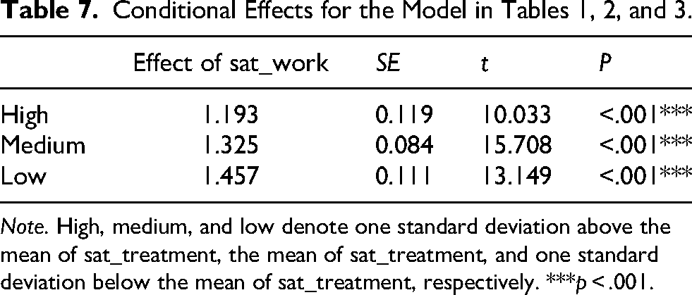
Note. High, medium, and low denote one standard deviation above the mean of sat_treatment, the mean of sat_treatment, and one standard deviation below the mean of sat_treatment, respectively. ***p < .001.

This second solution has the advantage that it directly assesses the magnitude of the moderation effect in an accessible way, without relying on the significance test results. Researchers can use the range of conditional effects to judge whether it is appropriate to run the risk of a Type II error (failing to detect a moderation effect) and model misspecification, and drop the product term when it is not significant. It also prevents misinterpreting the coefficient of X as an unconditional effect or the main effect because it highlights the fact that the effect of X in this moderated regression model depends on W, whether XW is significant or not.

The third solution is mean-centering. Although, as argued by Hayes (2022), mean-centering is optional and is not a must, it has the advantage that, if it is done, the coefficient of X is the effect of X when W is equal to its mean. This conditional effect is invariant to the scaling of W. This makes the coefficient of X, the so-called main effect, interpretable, even if the model without the product term is not reported (e.g., Milgramm et al., 2021). We must stress that the coefficient of X is a conditional effect even with mean-centering. Nevertheless, in this case, we still recommend calling this effect the weighted average conditional effect (Hayes et al., 2012) of X if W is discrete and takes only a limited number of values, or simply the effect of X when W is equal to its mean, rather than the main effect. Otherwise, readers need to check whether the moderator is mean-centered or standardized to interpret the main effect correctly.

Recommendations

If the moderation effect is judged to be absent, we recommend one of three options: (1) reporting on the model without the product term and interpreting the coefficient of the focal variable X in the model; (2) reporting the conditional effects of X to demonstrate the lack of moderation; or (3) reporting the coefficient of X as the effect of X when W is equal to its mean if W is mean-centered (or standardized). Given the strong conventions, we believe that it is acceptable to call the coefficient of the focal variable in a moderated regression model the main effect so long as it is made clear in the study that the coefficient of X is interpreted as a conditional effect.

Calling the coefficient of X the main effect without making it clear how the coefficient is interpreted can lead to misleading conclusions, such as treating the conditional effect as the mean conditional effect when it is not (no mean-centering and no main-effect parameterization) or treating the conditional effect as the mean conditional effect as in ANOVA, when it is the weighted mean conditional effect that depends on the distribution of the moderator.

Visualizing the Conditional Effects

It is common for researchers to visualize the moderation effect by plotting two or three lines for the conditional effects of two or three different levels of the moderator. However, it is common for researchers to use the same range of X for all lines, such as one standard deviation below the mean to one standard deviation above the mean. This is appropriate when the distribution of X is the same or very similar for the different levels of the moderator. However, this may not be the case because it assumes that the moderator and the predictor are uncorrelated.

The tumble graph proposed by Bodner (2016) solves this problem by computing the endpoints of each line using sample statistics of X for a particular level of W. For example, if W is dichotomous, instead of using the mean and standard deviation of X in the full sample, the line for the effect of X when W = 0 is plotted using the mean and standard deviation of X in the group with W = 0. Similarly, the line for the effect of X when W = 1 is plotted using the mean and standard deviation of X in the group with W = 1.

Suppose we explore how the effect of age on self-rated success is moderated by gender. Solely for the sake of illustration, we created a copy of the data set (dat2) and removed cases to create an association between age and gender (for details, see the code on the Open Science Framework page). The regression results are shown in Table 8.

Table 8.
Moderated Regression—Unstandardized—Categorical Moderator.

B SE t P

Constant 5.06 0.36 14.19 <.001*

Age 0.01 0.01 0.93 .354

Gender −0.70 0.61 −1.14 .255

Age × gender 0.03 0.01 2.36 .019

Note: * p < .001.

The left panel of Figure 2 is an example of a typical graph generated by the plot method for cond_effects() using the manymome package:
cond_out8 < - cond_effects(wlevels = “gender”,

y = “success”,

x = “age”,

fit = lm_out8)

plot(cond_out8)

Figure 2.
Plots for Conditional Effects: Gender.

This graph gives the impression that the age ranges are the same for males and females. The right panel is a tumble graph generated by the following code:

plot(cond_out8,

graph_type=“tumble”)

It shows that the two gender groups do not have identical age distributions. The female group has a lower mean age and a smaller standard deviation of age than the male group. Note that this difference in standard deviation, alone, does not violate any assumptions in OLS regression because the assumption of homogeneity of variance is on the conditional variance of the error term, not on the predictors (Fox, 2019).

Suppose that the mean and standard deviation of X are indeed similar in the two groups. In this case, the tumble graph will be similar to the typical graph plotted using the full sample mean and standard deviation of X. One drawback of the tumble graph is the smaller sample sizes used to estimate the means and standard deviations of X for the groups. Therefore, if the tumble graph does not reveal substantial differences in the means and standard deviations of X, researchers can resort to the typical graph, using the same mean and standard deviation for all the line segments. However, if the mean and/or standard deviation of X is different, as in the example above, a tumble graph is preferred, especially when the differences are theoretically meaningful or can highlight a limitation in the sample (e.g., a difference in the age distributions between the two groups, as in Figure 2).

If W is continuous, researchers need to select a method to estimate the mean and standard deviation conditional on the value of W. Bodner (2016) proposes regressing X on W and using the estimated standard deviation of the error term. Cheung et al. (2022) adopted a nonparametric method and used the 16 percentiles of cases within the value of W (e.g., if the value of W corresponded to the 25th percentile of the distribution of W, cases from the 9th to the 31st percentile were selected) to compute the mean and standard deviation of X. Whatever the implementation, it is always a good idea to first use a variant of the tumble graph instead of using the full sample mean and standard deviation of X to see whether there are substantial differences in the distributions of X for different values of W. An example of a tumble graph for a continuous moderator is shown in the right panel of Figure 3, with a typical plot of the same model presented in the left panel for comparison. Like the previous example, the tumble graph reveals that higher satisfaction with education (sat_edu, the moderator) is associated with higher satisfaction with medication (sat_med, the focal variable).

Figure 3.
Plots for Conditional Effects: Satisfaction with Education.

Recommendations

It is recommended that a variant of a tumble graph is used to visualize the conditional effects, unless the correlation between X and W is nearly zero in the sample, or the distributions of X are similar for the different values of W selected to plot the conditional effects.

Suppose that a conventional graph of simple effects is used, and X and W are correlated. In this case, the pattern of the moderation in the graph can be misleading, such as showing incorrectly that cases have an identical distribution (mean and standard deviation) on X in the two groups (the left panel of Figure 2) when cases in one group tend to be higher on X than cases in the other group (the right panel of Figure 2). This association between X and W can be a limitation in the sampling, which should be presented as a finding for discussion.

Standardization

There are situations when it is helpful to interpret the coefficients with one or more variables standardized. We discuss below several cases in which the analysis and interpretation can be improved in these situations.

All Variables Standardized and W Continuous

We found that some studies report only the standardized coefficients, and not the unstandardized coefficients. This can and should be done if the changes in the variables, and hence the effects of the variables on the outcome variable, are more interpretable when they are standardized. However, it is well known that it is inappropriate to report the coefficient of the product term when this term is standardized (Hayes, 2022), or, if it is reported, this coefficient should “never be interpreted [emphasis in original]” (Hayes, 2022, p. 333). This is because, when standardized, the term Z_XW is no longer a product term and so can no longer be interpreted as a change in the effect of the predictor when the moderator changes:
$Z_{Y} = B_{0}^{'} + B_{X}^{'} Z_{X} + B_{W}^{'} Z_{W} + B_{X W}^{'} Z_{X W} + e$

First, the coefficient of the standardized product term is nearly always a biased estimate of the correct standardized moderation effect, the coefficient of Z_XZ_W, denoted as $B_{Z_{X} Z_{W}}$ (Cheung et al., 2022). Cheung et al. (2022) show that, assuming a multivariate normal distribution of the predictors (X and W), the population value of $B_{X W}^{'}$ is $\sqrt{1 + ρ_{X W}^{2}} B_{Z_{X} Z_{W}}$ , where $ρ_{X W}^{2}$ is the population correlation between X and W. Therefore, $B_{X W}^{'}$ tends to be larger than $B_{Z_{X} Z_{W}}$ , unless X and W are uncorrelated.

Second, the coefficient of Z_X is also not the standardized effect of X when Z_W = 0, unless mean-centering is done in doing regression, because Z_W = 0 when W is equal to its mean. Therefore, the coefficients reported by a program that standardizes all variables after the product term is formed yield misleading coefficients, or at least coefficients that are difficult to interpret.

Suppose we use satisfaction with medication to predict self-rated success, and satisfaction with education as the moderator. Table 9 shows the unstandardized estimates, with the usual standardized coefficients (with the product term standardized) included—computed by the function lm.beta() from the R package lm.beta—presented in the column “β (all terms standardized).”

Table 9.
Moderated Regression—All Terms, Including the Product Terms, Standardized.

B β (all terms standardized) β (Aiken & West) t p

Constant 4.81 −0.014 5.39 <.001***

sat_med 0.06 0.016 0.158 0.24 .814

sat_edu −0.37 −0.114 0.069 −1.22 .223

sat_med × sat_edu 0.17 0.262 0.039 2.01 .045*

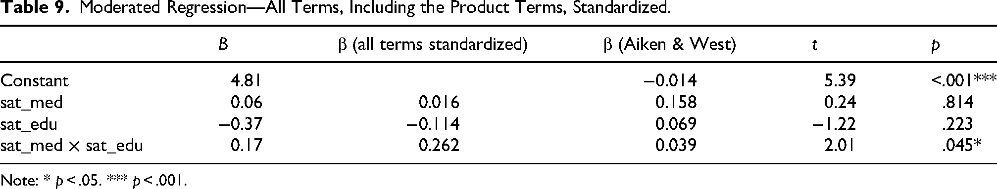
Note: * p < .05. *** p < .001.

The results with standardization done correctly, as suggested by Aiken and West (1991), using the function std_selected() from the stdmod package, are presented in Table 9 in the column “β (Aiken & West).” The function std_selected() accepts the output of lm() and updates the results by standardizing the selected variables. However, it does the standardization before forming the product term, as suggested by Aiken and West (1991). The coefficients of the product term differ substantially: .039 if standardized correctly and .262 in the incorrect standardized solution. Only the coefficient in the second solution (Aiken & West) can be interpreted correctly as an increase in the standardized effect of satisfaction with medication when satisfaction with education increased by one standard deviation, as demonstrated by the three conditional effects of satisfaction with medication computed by the function cond_effect() from stdmod, with all variables standardized (Table 10).⁷

Table 10.
Conditional Effects With All Variables Standardized.

Effect of sat_med Change in effect when sat_edu increases by 1 SD

High 0.197 0.197 – 0.158 = 0.039

Medium 0.158 0.158 – 0.119 = 0.039

Low 0.119

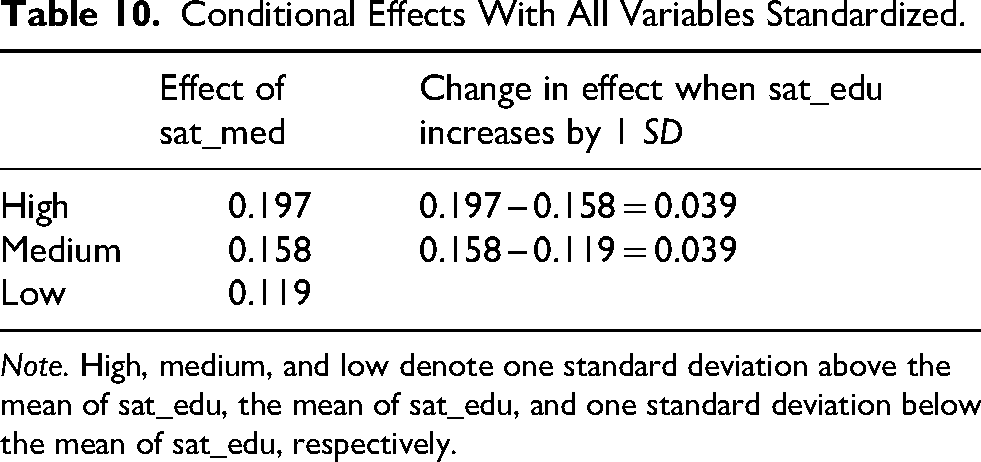
Note. High, medium, and low denote one standard deviation above the mean of sat_edu, the mean of sat_edu, and one standard deviation below the mean of sat_edu, respectively.

As shown in Table 10, when the standardized moderator (sat_edu) increased by one unit (i.e., one standard deviation), the standardized effect of the focal variable (sat_med) increased by .039, which is the coefficient of the product term when standardization is conducted correctly. Therefore, if researchers deem that their results are more interpretable when X, Y, and/or W are standardized, they should be standardized before forming the product term. Common tools that perform standardization without taking into account the product terms should never be used to compute the standardized solution. In the studies reviewed, some correctly standardized the variables first (e.g., Chen et al., 2021; Wen et al., 2023). However, for other studies that reported a standardized solution, it is not clear whether standardization was conducted as suggested in the moderated regression analysis.

Recommendation

It is recommended that the product term should never be standardized. If standardization is meaningful and preferred, it should be carried out before computing the product term, and this should be clearly stated in the study. If the product term is standardized, the coefficient of the product term can no longer be interpreted meaningfully because the term is no longer a product term and cannot be interpreted as the change in the effect of X when the moderator W changes.

All Variables Standardized and W Dichotomous

We also found that, when moderators are dichotomous, they are also sometimes standardized. It has been argued that dummy variables should almost never be standardized (Darlington & Hayes, 2016). If standardized, their means and standard deviations depend on the distribution of the group frequencies. Even if done as presented above for continuous W, the coefficient of the product term is still not interpretable. The meaning of the product term is unclear. Moreover, it certainly does not make sense to talk about a one-standard-deviation increase of the dummy variable.

Suppose we use the number of family members with autism (fam) to predict self-rated success, and gender as the moderator (male = 0, female = 1). The results, with the usual standardized estimates, are presented in Table 11.

Table 11.
Moderated Regression—All Terms, Including the Product Terms and the Dummy Variable, Standardized.

B β (all terms standardized) β (Aiken & West) t p

Constant 5.40 0.032 45.81 <.001*

fam 0.22 0.131 0.131 4.88 <.001*

gender 0.09 0.015 −0.103 0.43 .669

fam × gender −0.19 −0.090 −0.111 −2.34 .019*

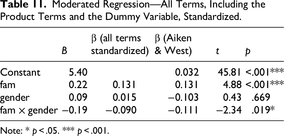
Note: * p < .05. *** p < .001.

The coefficient of the product term is −0.19. However, it is not interpretable. The column “β (Aiken & West)” shows the estimates with all but gender standardized. The coefficient is −0.111, which is different from −0.090 on the standardized metrics. This coefficient can be correctly interpreted as the difference in the standardized effect of the number of family members with autism on self-rated success. The conditional effects generated by the cond_effect() function from stdmod are shown in Table 12. The difference in the effect is 0.111, the coefficient of the product term when standardization was conducted appropriately.

Table 12.
Conditional Effects With All Variables, Except for Gender, Standardized.

Effect of fam Difference in the conditional effect

Female 0.020 0.020 –0.131 = −0.111

Male 0.131

Recommendation

If the moderator is dichotomous, it should never be standardized. If it must be standardized, it should be ensured that the coefficient, even if reported, is not interpreted. If the dichotomous moderator is standardized, the coefficient of the product term is not interpretable because it is not the difference in the effect of X between the two groups.

The focal variable (X) and the outcome variable (Y) can be standardized, if necessary. How the standardization was conducted should be reported clearly.

CIs

Another issue that has gained increasing attention from methodologists over the last decade is forming appropriate CIs for the coefficient when the variables are standardized. Yuan and Chan (2011) show analytically that the OLS standard errors, and hence CIs, of the regression coefficients when variables are standardized are biased, partly because they do not take into account the sampling variance in the standardizer (the standard deviations). This affects the results even when standardization is done correctly. We are not aware of studies discussing this issue in moderation. However, it can be shown that the standardized moderation effect can be computed from the unstandardized moderation effect (e.g., Cheung et al., 2022):
$B_{z_{X} z_{W}} = B_{X W} (\frac{S D_{X} S D_{W}}{S D_{Y}})$

Therefore, it can be inferred that the standardized moderation effect is similarly biased if the OLS standard error is used. This means that, even if researchers have performed standardization correctly, the CIs cannot be trusted.

We are not aware that any analytical solution has been proposed for forming the standard error correctly for the standardized moderation effect. The existing solution assumes that the variables are multivariate normal and/or the standardized coefficient is computed from two standard deviations. The former assumption is violated because the product term would not be normally distributed even if X and W were jointly multivariate normal (Craig, 1936). Second, the standardized moderation effect involves three, not two, standard deviations. Extending Yuan and Chan’s (2011) suggestion, we propose using bootstrapping to form CIs when standardization is done in moderation, with standardization repeated in each bootstrap sample to take into account the sampling error in the standard deviations.

For the sake of illustration, we selected 100 cases from the full sample to make the difference more noticeable. We used the function std_selected_boot() from the stdmod package to form a percentile nonparametric bootstrap CI for the coefficients after standardization. The results are shown in Table 13.

Table 13.
Moderated Regression—Unstandardized with Bootstrap CI.

β (Aiken & West) Bootstrap 95% CI OLS 95% CI based on t statistic

Constant −0.081 [−0.184, −0.006] [−0.0277, 0.115]

sat_med 0.287 [0.085, 0.495] [0.086, 0.489]

sat_edu 0.009 [−0.218, 0.210] [−0.189, 0.207]

sat_med × sat_edu 0.281 [0.038, 0.493] [0.085, 0.476]

In general, the OLS CIs are narrower than those based on bootstrapping. However, they are biased (Yuan & Chan, 2011) because they ignore the sampling error in the standardizers (the standard deviations of the variables)—that is, they underestimate the sampling variation in the coefficients after standardization. The bootstrap CIs are wider because they take into account the sampling variation of the standard deviations by repeating the standardization in each bootstrap sample.

Some studies of moderation, usually moderated mediation, used bootstrapping CIs after the variables were standardized (e.g., Rakap & Vural-Batik, 2024). Although bootstrapping was used, this cannot address the problem presented above because the standardization was conducted only once, not in each bootstrap sample. Although we are not aware of empirical studies on this issue in moderation, research has shown that standardization before bootstrapping can lead to suboptimal CIs in mediation (Cheung, 2009). We believe that the same problem can occur in moderation if standardization is conducted only once.

Recommendation

If CIs are needed for moderated regression involving standardization, bootstrapping CIs should be reported in place of OLS CIs, with standardization conducted in each bootstrap sample, or other analytic solutions that take into account the sampling error in the standardizers. If OLS CIs are reported, the intervals are biased because they ignore the fact that the standard deviations are sample estimates. The CI can be either too wide or too narrow. If too narrow, OLS CIs are too optimistic about the sampling variation of the standardized coefficients.

Conclusion

It is not our intention to suggest that the researchers in the selected area we reviewed did anything wrong intentionally. Moreover, most of the problems presented above can also be found in other areas of psychology, partly because of the complexity of moderation analysis and partly due to the default behaviors of popular statistical tools. In many cases, we found that the major problem was having insufficient information to determine whether the analysis was conducted correctly. The availability of statistical tools for computing and visualizing conditional effects partly solves some of the problems, such as reporting conditional effects easily with the PROCESS macro (Hayes, 2022). However, as long as regression coefficients are reported, some of the problems remain. We hope that our discussion and explanation here can help researchers in psychology conduct and report moderation effects more effectively. More tools would be beneficial, but researchers are ultimately responsible for doing the analysis right and interpreting the results accurately.

	B	SE	t	p
Constant	1.329	0.325	4.093	<.001***
sat_work	1.357	0.095	14.249	<.001***
gender	−0.509	0.613	−0.830	.406
sat_work × gender	0.073	0.181	0.405	.686

	B	SE	t	p
Constant	0.820	0.520	1.576	.115
sat_work	1.430	0.154	9.313	<.001***
gender	−0.509	0.613	−0.830	.406
sat_work × gender	−0.073	0.181	0.405	.686

	B	SE	t	p
Constant	1.074	0.307	3.504	<.001***
sat_work	1.393	0.090	15.425	<.001***
Gender	0.509	0.613	0.830	.406
sat_work × gender	−0.073	0.181	−0.405	.686

	B	SE	t	p
Constant	−0.091	0.715	−0.127	.899
sat_work	1.674	0.218	7.690	<.001***
sat_treatment	0.495	0.238	2.080	.038*
sat_work × sat_treatment	−0.117	0.069	−1.690	.091

	B	SE	t	p
Constant	0.404	0.505	0.800	.899
sat_work	1.557	0.156	9.980	<.001***
sat_treatment	0.495	0.238	2.080	.038*
sat_work × sat_treatment	−0.117	0.069	−1.690	.091

	B	SE	t	p
Constant	1.393	0.289	4.823	<.001***
sat_work	1.322	0.084	15.654	<.001***
sat_treatment	0.495	0.238	2.080	.038*
sat_work × sat_treatment	−0.117	0.069	−1.690	.091

	Effect of sat_work	SE	t	P
High	1.193	0.119	10.033	<.001***
Medium	1.325	0.084	15.708	<.001***
Low	1.457	0.111	13.149	<.001***

	B	SE	t	P
Constant	5.06	0.36	14.19	<.001***
Age	0.01	0.01	0.93	.354
Gender	−0.70	0.61	−1.14	.255
Age × gender	0.03	0.01	2.36	.019

	B	β (all terms standardized)	β (Aiken & West)	t	p
Constant	4.81		−0.014	5.39	<.001***
sat_med	0.06	0.016	0.158	0.24	.814
sat_edu	−0.37	−0.114	0.069	−1.22	.223
sat_med × sat_edu	0.17	0.262	0.039	2.01	.045*

	Effect of sat_med	Change in effect when sat_edu increases by 1 SD
High	0.197	0.197 – 0.158 = 0.039
Medium	0.158	0.158 – 0.119 = 0.039
Low	0.119

	B	β (all terms standardized)	β (Aiken & West)	t	p
Constant	5.40		0.032	45.81	<.001***
fam	0.22	0.131	0.131	4.88	<.001***
gender	0.09	0.015	−0.103	0.43	.669
fam × gender	−0.19	−0.090	−0.111	−2.34	.019*

	Effect of fam	Difference in the conditional effect
Female	0.020	0.020 –0.131 = −0.111
Male	0.131

	β (Aiken & West)	Bootstrap 95% CI	OLS 95% CI based on t statistic
Constant	−0.081	[−0.184, −0.006]	[−0.0277, 0.115]
sat_med	0.287	[0.085, 0.495]	[0.086, 0.489]
sat_edu	0.009	[−0.218, 0.210]	[−0.189, 0.207]
sat_med × sat_edu	0.281	[0.038, 0.493]	[0.085, 0.476]

Footnotes

ORCID iDs

Shu Fai Cheung

Mariana Aguiar

Funding

The authors disclosed receipt of the following financial support for the research, authorship, and/or publication of this article: This work was supported by the University of Macau (grant number MYRG-GRG2023-00155).

Declaration of Conflicting Interests

The authors declared no potential conflicts of interest with respect to the research, authorship, and/or publication of this article.

Data Availability Statement

The code and data used in this article are available in the Open Science Framework at

Notes

References

Aiken

L. S.

West

S. G.

(1991). Multiple regression: Testing and interpreting interactions. Sage.

Bodner

T. E.

(2016). Tumble graphs: Avoiding misleading end point extrapolation when graphing interactions from a moderated multiple regression analysis. Journal of Educational and Behavioral Statistics, 41(6), 593–604. https://doi.org/10.3102/1076998616657080

Chen

S. D.

X. K.

Chen

S. Q.

Ren

(2021). Parental self-efficacy and behavioral problems in children with autism during COVID-19: A moderated mediation model of parenting stress and perceived social support. Psychology Research and Behavior Management, 14, 1291–1301. https://doi.org/10.2147/prbm.s327377

Cheung

M. W.-L.

(2009). Comparison of methods for constructing confidence intervals of standardized indirect effects. Behavior Research Methods, 41(2), 425–438. https://doi.org/10.3758/BRM.41.2.425

Cheung

S. F.

Cheung

S.-H.

(2024). manymome: An R package for computing the indirect effects, conditional effects, and conditional indirect effects, standardized or unstandardized, and their bootstrap confidence intervals, in many (though not all) models. Behavior Research Methods, 56(5), 4862–4882. https://doi.org/10.3758/s13428-023-02224-z

Cheung

S. F.

Cheung

S.-H.

Lau

E. Y. Y.

Hui

C. H.

Vong

W. N.

(2022). Improving an old way to measure moderation effect in standardized units. Health Psychology, 41(7), 502–505. https://doi.org/10.1037/hea0001188

Craig

C. C.

(1936). On the frequency function of xy. Annals of Mathematical Statistics, 7(1), 1–15. https://doi.org/10.1214/aoms/1177732541

Darlington

R. B.

Hayes

A. F.

(2016). Regression analysis and linear models: Concepts, applications, and implementation (Illustrated edition). The Guilford Press.

Deserno

M. K.

Borsboom

Begeer

Geurts

H. M.

(2017). Multicausal systems ask for multicausal approaches: A network perspective on subjective well-being in individuals with autism spectrum disorder. Autism, 21(8), 960–971. https://doi.org/10.1177/1362361316660309

10.

Fox

(2019). Regression diagnostics: An introduction (2nd ed.). Sage.

11.

Friedrich

R. J.

(1982). In defense of multiplicative terms in multiple regression equations. American Journal of Political Science, 26(4), 797–833. https://doi.org/10.2307/2110973

12.

Haslbeck

J. M. B.

Waldorp

L. J.

(2020). mgm: Estimating time-varying mixed graphical models in high-dimensional data. Journal of Statistical Software, 93(8), 1–48. https://doi.org/10.18637/jss.v093.i08

13.

Hayes

A. F.

(2022). Introduction to mediation, moderation, and conditional process analysis: A regression-based approach (3rd ed.). Guilford Press.

14.

Hayes

A. F.

Glynn

C. J.

Huge

M. E.

(2012). Cautions regarding the interpretation of regression coefficients and hypothesis tests in linear models with interactions. Communication Methods and Measures, 6(1), 1–11. https://doi.org/10.1080/19312458.2012.651415

15.

Hollocks

M. J.

Wood

J. J.

Storch

E. A.

Cho

A.-C.

Kerns

C. M.

Kendall

P. C.

(2023). Reward sensitivity predicts the response to cognitive behavioral therapy for children with autism and anxiety. Journal of Clinical Child & Adolescent Psychology, 52(6), 811–818. https://doi.org/10.1080/15374416.2022.2025596

16.

Lash

T. L.

VanderWeele

T. J.

Haneuse

Rothman

K. J.

(2021). Modern epidemiology (4th ed.). Wolters Kluwer.

17.

Little

T. D.

(2013). Longitudinal structural equation modeling. Guilford Press.

18.

Liu

Zhang

Liu

Yin

(2024). The relationship between parenting stress and parental burnout among Chinese parents of children with ASD: A moderated mediation model. Journal of Autism and Developmental Disorders, 54(4), 1527–1537. https://doi.org/10.1007/s10803-022-05854-y

19.

Milgramm

Christodulu

K. V.

Rinaldi

M. L.

(2021). Brief report: Predictors of teacher-rated academic competence in a clinic sample of children with and without autism spectrum disorder. Journal of Autism and Developmental Disorders, 51(6), 2132–2138. https://doi.org/10.1007/s10803-020-04680-4

20.

Nutor

Dunlop

Sadler

Brennan

P. A.

(2024). Prenatal cannabis use and offspring autism-related behaviors: Examining maternal stress as a moderator in a Black American cohort. Journal of Autism and Developmental Disorders, 54(6), 2355–2367. https://doi.org/10.1007/s10803-023-05982-z

21.

Park

S.-J.

(2023). Decomposing main effects in moderated regression models. Journal of Business Research, 157, Article 113577. https://doi.org/10.1016/j.jbusres.2022.113577

22.

Rakap

Vural-Batik

(2024). Mitigating the impact of family burden on psychological health in parents of children with special needs: Buffering effects of resilience and social support. Journal of Applied Research in Intellectual Disabilities, 37(1), Article e13179. https://doi.org/10.1111/jar.13179

23.

R Core Team. (2024). R: A language and environment for statistical computing. R Foundation for Statistical Computing. https://www.R-project.org/

24.

Tabak

B. A.

Young

K. S.

Torre

J. B.

Way

B. M.

Burklund

L. J.

Eisenberger

N. I.

Lieberman

M. D.

Craske

M. G.

(2020). Preliminary evidence that CD38 moderates the association of neuroticism on amygdala-subgenual cingulate connectivity. Frontiers in Neuroscience, 14, Article 11. https://doi.org/10.3389/fnins.2020.00011

25.

Wen

Ren

Chen

(2023). Parents’ personality, parenting stress, and problem behaviors of children with special needs in China before and during the COVID-19 pandemic. Current Psychology, 42(31), 27305–27316. https://doi.org/10.1007/s12144-022-03869-3

26.

Yoder

P. J.

Stone

W. L.

Edmunds

S. R.

(2021). For which younger siblings of children with autism spectrum disorder does parent-mediated intervention work? Autism, 25(1), 58–69. https://doi.org/10.1177/1362361320943373

27.

Yuan

K.-H.

Chan

(2011). Biases and standard errors of standardized regression coefficients. Psychometrika, 76(4), 670–690. https://doi.org/10.1007/s11336-011-9224-6

28.

Zhang

Lin

Zhou

Zhang

Xiong

(2024). Social support and parenting self-efficacy in parents of children with ASD: The mediating role of post-traumatic growth and the moderating role of self-esteem. Current Psychology, 43(10), 9025–9040. https://doi.org/10.1007/s12144-023-05031-z

Doing,Reporting,and Interpreting Moderation Right: Recommendations for Selected Common Practices

Abstract

Keywords

A Brief Description of Moderation Conducted by Multiple Regression

A Systematic Review of Moderation Analysis in Studies on Autism Spectrum Disorder

Doing and Reporting Moderation Right (and How To Do It Wrong)

Unstandardized Solution

Interpreting the So-Called Main Effect (Especially When the Product Term Is Not Significant)

When Both X and W Are Dichotomous

When X is Numerical and W is Dichotomous

When Both X and W are Numerical

Summary

Recommendations

Visualizing the Conditional Effects

Recommendations

Standardization

All Variables Standardized and W Continuous

Recommendation

All Variables Standardized and W Dichotomous

Recommendation

CIs

Recommendation

Conclusion

Footnotes

ORCID iDs

Funding

Declaration of Conflicting Interests

Data Availability Statement

Notes

References