
Abstract
Knee osteoarthritis (OA) is a prevalent and disabling disease that can develop over decades. This disease is heterogeneous and involves structural changes in the whole joint, encompassing multiple tissue types. Detecting OA before the onset of irreversible changes is crucial for early management, and this could be achieved by allowing knee tissue visualization and quantifying their changes over time. Although some imaging modalities are available for knee structure assessment, magnetic resonance imaging (MRI) is preferred. This narrative review looks at existing literature, first on MRI-developed approaches for evaluating knee articular tissues, and second on prediction using machine/deep-learning-based methodologies and MRI as input or outcome for early OA diagnosis and prognosis. A substantial number of MRI methodologies have been developed to assess several knee tissues in a semi-quantitative and quantitative fashion using manual, semi-automated and fully automated systems. This dynamic field has grown substantially since the advent of machine/deep learning. Another active area is predictive modelling using machine/deep-learning methodologies enabling robust early OA diagnosis/prognosis. Moreover, incorporating MRI markers as input/outcome in such predictive models is important for a more accurate OA structural diagnosis/prognosis. The main limitation of their usage is the ability to move them in rheumatology practice. In conclusion, MRI knee tissue determination and quantification provide early indicators for individuals at high risk of developing this disease or for patient prognosis. Such assessment of knee tissues, combined with the development of models/tools from machine/deep learning using, in addition to other parameters, MRI markers for early diagnosis/prognosis, will maximize opportunities for individualized risk assessment for use in clinical practice permitting precision medicine. Future efforts should be made to integrate such prediction models into open access, allowing early disease management to prevent or delay the OA outcome.
Keywords
Introduction
Although cartilage degradation characterizes knee osteoarthritis (OA), this disease is now recognized as heterogeneous and involves tissues of the whole joint. It engenders pain, reduces the quality of life and mobility, increases the risk of comorbidities, and often results in the need for joint replacement. OA is on the rise globally, with its prevalence increasing by about 113% from 1990 to 2019. 1 Such growth could reflect that it is not only older individuals affected by this disease but also younger individuals. This is evidenced by the report showing that more than eight million knee OA patients in the United States are younger than 65 years old, including two million less than 45 years old. 2
Traditionally viewed as a disease characterized by a slow progression, recent work suggests a more nuanced model of the natural history of OA. Although its evolution could be slow and have a silent progression, the disease progression and severity could occur rapidly for some individuals.3–6 Yet, with the current tools, OA is usually diagnosed, at the earliest, at the moderate stages of the disease process when preventive measures are more complex for the patient to apply and, if so, often with limited success. The current approaches to early OA detection, which use demographic and clinical parameters with sometimes adjunct radiography, are imperfect in providing a specific and sensitive diagnosis. It is believed that pre-symptomatic disease detection could be achieved by evaluating the deterioration and progression of the knee structure. It is, therefore, essential to visualize and quantify the knee tissues involved in the disease and their changes over time.
Biomarkers are an excellent option as they could be used early during the disease process – before serious joint damage. At present, a variety of fluid biomarkers have been proposed to detect knee OA.7,8 However, fluid biomarkers capable of providing an accurate early diagnosis or predicting disease progression still require further mining as the majority lack sensitivity and specificity for diagnosing, predicting, and monitoring the disease.
Joint imaging has attracted ever-growing attention in OA biomarker research. Different image modalities can be used to assess articular tissue, including, among others, ultrasound, radiography, and magnetic resonance imaging (MRI). Although for some of these techniques, advantages have been shown in one over another, their disadvantages limit their common use in exploring the early changes in joint tissues.
Ultrasound is a non-invasive and easily accessible method that permits the visualization of the superficial soft tissue structures surrounding the knee, including tendons, ligaments, muscles, and synovial fluid. However, it does not allow visualizing cartilage damage, the cruciate ligament, as well as the entirety of the meniscus. In addition, it is highly operator dependent, which could induce bias.
Although regulatory agencies still recognize radiography as the gold standard for disease-modifying osteoarthritis drug (DMOAD) trials, it has many constraints that considerably limit its use. Among several significant limitations, this technique does not yield information on early OA or the cartilage itself but provides only one measurement, that is, joint space width. Moreover, it does not allow for the visualization of many joint tissues and has a weak sensitivity to change. Also, a large number of patients are required for an extended follow-up period to achieve reliable results in DMOAD trials.
MRI, in addition to permitting direct tissue visualization of joint tissue structures, is non-invasive, objective, reproducible, sensitive to change, and quantitative knee tissues and their changes over time in the same patients can be determined reliably. This technology also allows the detection of knee tissue alterations before radiographic evidence, in which MRI may show disease manifestations even with normal radiographs. Another advantage is that it can reveal the three-dimensional (3D) structure of the knee joint tissues, thus providing a better interpretation of the OA condition with a more detailed structure of the knee. In short, this technology is an unbiased approach to the comprehensive profiling of knee structural markers.
In the first part, we will depict the MRI processing approaches that allow visualization and quantification of many knee articular tissues. Evaluating knee structures with MRI may provide a compelling alternative and could act as a sensor for disease determinants.
Predictive models/tools for an early diagnosis and prognosis are essential to guide clinicians by estimating a patient’s risk. In the past, developing a model/tool to predict early or progressive OA had been hindered by a lack of appropriate techniques for reducing and interpreting large volume and multidimensional OA data. Recently, artificial intelligence has been widely used in medicine and healthcare, and one of its main areas is machine/deep learning for data classification, identifying patterns, and prediction. Machine learning refers to a series of mathematical algorithms inspired by the structure and function of the brain that enables the machine to ‘learn’ the relationship between input/features and output/outcome data. Deep learning is a subfield of machine learning, and the term ‘deep’ refers to the number of layers through which the data are transformed. Deep-learning-based models can be used in situations involving more than two classes. Such methodology has improved the ability to predict the risk of complex diseases, and models or algorithms have been developed for the diagnosis and prognosis of many conditions. The last part of this review summarizes the research progress in predicting the early diagnosis and prognosis of knee OA using machine/deep learning and MRI data.
MRI assessments enabling visualization and quantification of knee structures and their alterations
Although cartilage degradation is the hallmark of OA, it does not occur at an early stage of the disease process. Other knee tissue alterations precede the onset of radiographic knee OA.9–13 Therefore, to diagnose early OA, we should be able to assess many tissues of the knee. MRI technology provides high-resolution images that detect soft tissues and osseous structures, allowing their visualization. The MRI knee tissue evaluation methods include scoring and manual, semi-automated and fully automated quantitative systems. This section overviews the assessments used for different knee tissue segmentation, which have rendered possible the quantification of their alterations as well as change over time in the same patients. The knee tissues reviewed here included cartilage, bone marrow lesions (BMLs), bone shape/curvature, osteophytes, menisci, infrapatellar fat pad, effusion/synovial membrane, muscle, and ligaments. Of note, MRI sequences and protocols are not described as this topic is beyond the aim of this review.
Semi-quantitative scoring assessment
Global knee
The most used global knee MRI scoring techniques are the Whole-Organ MRI Score (WORMS), 14 Boston Leeds Osteoarthritis Knee Score (BLOKS), 15 MRI OsteoArthritis Knee Score (MOAKS), 16 and Knee Osteoarthritis Scoring System (KOSS). 17 They all consider many features and regions of the knee, providing a global assessment of the articulation and a comprehensive evaluation of the knee lesions cross-sectionally and longitudinally.
WORMS considers articular features such as cartilage, BMLs, osteophytes, meniscal as well as cruciate and collateral ligament damages, synovitis/effusion, intra-articular loose bodies, and peri-articular cysts/bursitis providing whole-organ multi-feature assessment. BLOKS evaluates BMLs, cartilage, osteophytes, synovitis, and effusions in nine regions. The MOAKS system further refines BML, cartilage, and meniscal morphology scoring. To detect longitudinal structural changes with higher sensitivity, ‘within-grade’ scores have been introduced and used to record changes observed between time points that do not fulfil the original integer grading scale criteria. 18 KOSS scores the presence of cartilaginous and osteochondral defects, osteophytes, subchondral cysts, bone marrow oedema and meniscal abnormalities in different compartments, as well as the presence and size of joint effusion, synovitis, and Baker’s cyst.
Single knee tissue
There have also been scoring systems developed for a single knee tissue alteration.
Cartilage defects
The evaluation of cartilage defects mainly uses the modified Outerbridge classification at medial and lateral tibial and femoral sites. Calculation is performed as the total of sub-regional scores. 19 Cartilage is considered normal if it has a uniform thickness. Cartilage defects include focal blistering and intra-cartilaginous areas of low signal intensity, irregularities on the surface, and deep ulceration.
Bone marrow lesions
BMLs are discrete areas of increased signal adjacent to the subcortical bone at the medial and lateral tibial and femoral sites. A scoring method considers the percentage of a subregion affected by BMLs (lesion size).14,20
Two primary bone lesions were typically observed: a hazy hyper white signal named oedema and a white sharply delimited hyper signal called a cyst (Figure 1).

Subchondral bone oedema and cyst. (a) Subchondral bone oedema in the femoral condyle and (b) cyst in the patella in human osteoarthritis knees using 3D sagittal fast imaging with steady-state precession with fat suppression MRI sequence.
Bone oedema is described as swelling within the bone. It can result from either a direct injury to the bone or a load-bearing greater than what can be sustained by the bone. It can also be found secondary to an inflammatory bone injury. Indeed, the histopathology of oedema describes various alterations, namely hypervascularity, cellular infiltration, bone marrow bleeding, fibromyxomatous transformation, trabecular alterations, and microfractures. 22 The cyst is a fluid-filled hole that develops inside a bone. It is identified as foci of a markedly increased MRI signal in the subchondral bone with well-delineated margins and no evidence of internal marrow tissue. 23 Generally, these structures (oedema and cyst) are both included in the scoring.
Meniscal alterations
The meniscus plays a critical role in shock absorption and is important in regulating load-bearing distribution. Alterations of this tissue are associated with knee OA pathogenesis and include extrusion, tear, and degeneration (Figure 2).

Meniscal pathologies.
The meniscal extrusion is a partial or total displacement of the meniscus of the tibial plateau and the tibial articular cartilage. The extent or percentage of meniscal extrusion is evaluated for the anterior, body, and posterior horns of the menisci.24–26
Meniscal tears consist of vertical, radial, longitudinal, vertical/horizontal flaps, and complex (combination of horizontal, vertical, and radial) tears extending to both femoral and tibial surfaces. Horizontal tears show a slightly oblique course extending out through the inferior surface of the meniscus, and complex tears are defined by a high signal that extends to three surfaces and three or more points. 25 It is assessed based on the presence of a signal, which is line shaped and brighter than the dark meniscus. It reaches the meniscus surface at both ends within six defined regions (anterior horn, body, and posterior horn at both medial and lateral tibiofemoral compartments). Several grading systems were proposed to measure the degree of meniscal tears. These included the proportion of the tears in meniscal areas (anterior, middle, and posterior horns),24,25 intrameniscal signal,27,28 index of suspicion, 29 and signal intensity and morphological abnormalities. 30
Meniscal degeneration is defined as an abnormal intrasubstance of grey signal intensity on MRI in which the proportion of the overall meniscus is graded.24,25
Infrapatellar fat pad
The infrapatellar fat pad is recognized as an important key player in OA and was recently considered an early marker for this disease’s incidence and progression.12,13 In MRI, the infrapatellar fat pad structure appears hypointense with lower signal foci throughout the tissue. Scoring methods were developed for the infrapatellar fat pad signal intensity, in which two are measured, the hypointense and hyperintense signals. It has been suggested that the hypointense signal relates to fibrosis and the hyperintense to inflammation.31–33 Compared to the hyperintense signal, limited studies have examined the hypointense signal. For the latter, the method counted MRI slices only where this signal was present. 34 The hyperintense signal used mainly a scoring method included in the MOAKs 16 and assessed as normal, mild, moderate, and severe. Another consists of a score from the percentage of signal intensity alteration in this tissue. 35
Effusion–synovitis
Knee effusion is the presence of synovial fluid in the intra-articular space of the joint. The effusion–synovitis scoring is performed in each subregion individually and estimated based on the maximal distention of the synovial cavity.14,17 Another evaluation of the effusion–synovitis volume uses the suprapatellar pouch and other cavities according to the intra-articular fluid-equivalent signal on an MRI, section-by-section basis. 36
Anterior cruciate ligament injury/tear
The anterior cruciate ligament (ACL) is one of the ligaments connecting the femur and tibia in the knee joint. It prevents anterior and posterior dislocation of the tibia and provides stability to the knee joint during rotation.37,38 It is the most injured major ligament of the knee, and, when injured, it induces a high risk of knee OA and tears in the meniscus and cartilage. 39 Ligament tears are scored as normal, partial, or complete. 40 The normal ligament displays a uniform low signal intensity and is continuous from the starting to the ending points. Indistinct ligament structures, local signal enhancement, visible oedema, and joint effusion around the ligament characterize partial tears. Complete tears appear as discontinuities or the disappearance of the ligament.
Quantitative techniques
While knee tissue scoring contributes to a better understanding of OA, it is time-consuming, based on ordinal scores, and requires expertise. Therefore, interest has grown in developing manual, semi-automated, and fully automated quantitative methods for several knee tissues.
Cartilage
Compositional MRI techniques
Quantitative MRI parametric mapping methodologies were developed to detect early changes in the biophysical and biomechanical properties of the cartilage matrix.Early cartilage modification includes increased water content, probably related to collagen damage and decreased glycosaminoglycan concentration and proteoglycan size. MRI modalities were developed to assess directly or indirectly this tissue’s glycosaminoglycan, water content, and the integrity of the collagen matrix. These included the diffusion-weighted imaging (DWI), 41 diffusion tensor MRI (DT-MRI), 42 glycosaminoglycan chemical exchange saturation transfer (gagCEST), 43 delayed gadolinium-enhanced MRI (dGEMRIC), 44 sodium imaging, 45 , T1, 46 T1ρ (or spin lock),47,48 T2 (or transverse relaxation time) (Figure 3),49,50 and T2* 51 relaxation times.
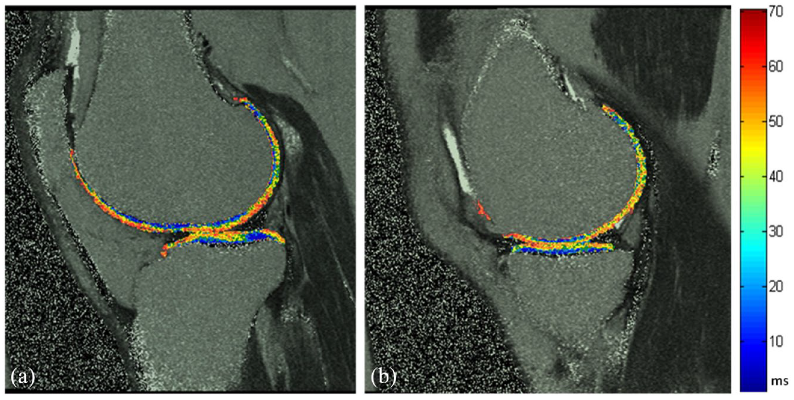
Cartilage T2 mapping. A representative T2 mapping assessment of the lateral (a) and medial (b) cartilage in a human osteoarthritis knee using a sagittal double echo steady-state MRI sequence for the cartilage delineation and a sagittal 2D multi-slice multi-echo MRI sequence for the cartilage assessment.
DWI is used for compositional cartilage assessment that evaluates the altered diffusion time of water within cartilage, in which water is more mobile in damaged cartilage, resulting in decreased diffusion times. DT-MRI provides information regarding the microstructure of the tissue and its anisotropy by tracking the local mobility of the water molecules in the tissue, which is used for displaying cartilage collagen fibre orientation. 52 The potential of the diffusion properties of cartilage using DWI and DT-MRI has been shown only in limited studies.42,53
The sodium content in cartilage is much higher than in the adjacent synovial fluid or bone, and quantitative sodium MRI has been shown to be highly specific for glycosaminoglycan content in cartilage. 54
The gagCEST and dGEMRIC are used for proteoglycans content measurement. However, experience in multicentre clinical trials is still limited for both sequences. For the dGEMRIC, this is probably because of the contrast enhancement that may lead to rare but potentially serious side effects, which has led to a warning from the U.S. Food and Drug Administration limiting its use. 55 The gagCEST is a technique based on the constant transfer of labile protons between solutes and water in a slow exchange regime. For better spectral separation and performance, a 7-Tesla magnetic resonance apparatus is preferred over a 3-Tesla, which has reduced sensitivity for granular assessment of very low glycosaminoglycan content. The challenge for multicenter clinical trials is that a 3-Telsa or lower field strength is generally used.
The most widely utilized quantitative MRI sequences to evaluate knee alterations are T1, T2, and T1ρ relaxation time.48,56–59 T1 relates to the measurement of the proteoglycan content, T2 with collagen network organization and structure and is directly associated with free water content, whereas T1ρ is sensitive to proteoglycan variations.46,49,50,60–62 It is suggested that T1ρ is well suited to differentiate the cartilage structure of healthy subjects from early OA patients and appeared more sensitive than T2 relaxation times. 63 T2* mapping provides more rapid acquisitions than T2 mapping, and although it has the potential for superior spatial resolution, it is limited by the greater sensitivity of magnetic field inhomogeneity. 51 Although they have good discriminative validity, limitations for using these techniques in clinical trials include standardization, in which inter-scanner variability is an important issue.64–66
In recent years, ultrashort echo time (UTE)-magnetic resonance sequences have been tested for quantitative assessment of the cartilage. UTE and UTE-T2* imaging mapping are quantitative techniques sensitive to changes in cartilage matrix architecture rather than composition.67,68 The combination of UTE-MRI with magnetization transfers (UTE-MT) and adiabatic T1ρ (UTE-Adiab T1ρ) sequences69,70 allows the quantification of the macromolecular content relative to water content in the tissue, supporting their potential for effective detection of cartilage degeneration.71,72 However, the association of early changes in knee tissues and OA incidence and progression with these sequences is yet to be demonstrated.
Cartilage volume and thickness
Quantitative systems were also developed for cartilage volume and average thickness.A manual knee cartilage volume quantitation was done by drawing disarticulation contours around the cartilage boundaries on a section-by-section basis. The volume of the cartilage plate was determined by summing the pertinent voxels within the resultant binary volume. 73 Such manual segmentation is time-intensive and generally restrictive to analyse only some knee regions.
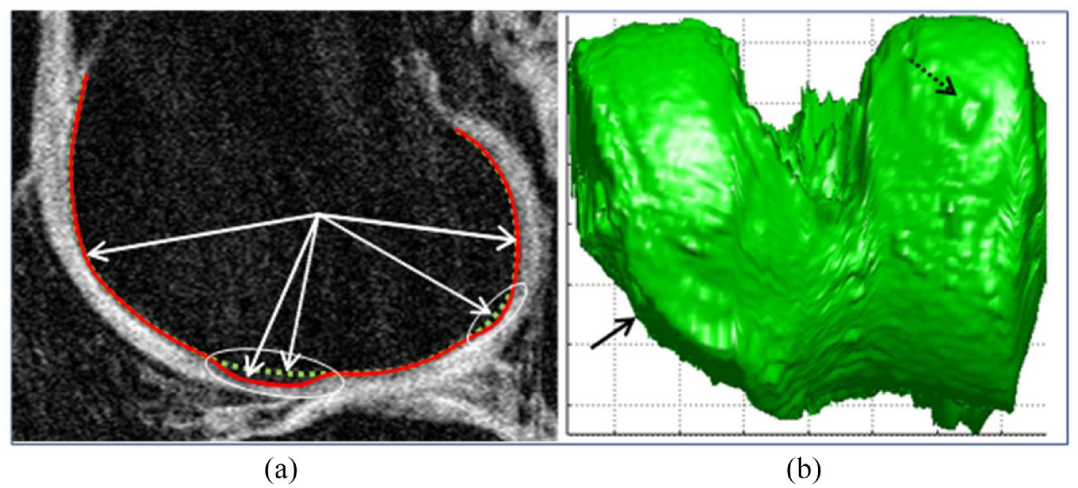
Semi-quantitative methods were also developed and used different modalities, including active contour and shape models,74–76 atlas-based models, 77 B-spline snakes, 78 graph cuts, 79 k-nearest neighbor, 80 and 3D Euclidean distance transformation. 81 After MRI acquisition, the segmentation is performed using pre-processing (noise removal, normalization, etc.), followed by extracting the cartilage surface and quantitative measurement. 81 Some of these systems first include segmenting the cartilage–synovial interfaces using a local coordinate system to map the corresponding cartilage geometry over time.75,82–84 Then, there was a delimitation of the bone–cartilage interfaces followed by an automatic initial continuous contour using 3D surface edges extracted from adjacent magnetic resonance slices, a delineation of the cartilage-soft tissue, and an automatic contour process using a 2D/3D active-contour process (snake) (Figure 4). 85 An active contour model-based method of segmenting the centre slice of consecutive MRI was proposed to minimize user interaction. 76 Also introduced were the gradient vector flow snakes, 86 embedding gradient directional information into the gradient vector flow snakes, 87 and the chessboard directional compensated gradient vector flow snakes. 88

Cartilage delineation and 3D volumetric representation. (a) Femoral condyle and tibial plateau contour delineation were performed semi-automatically, showing the cartilage inner and outer boundary permitting this tissue volume/thickness assessment in a human osteoarthritis knee. MRI sequence was a 3D sagittal fast imaging with steady-state-free precession with fat suppression. (b) 3D volumetric representation of the lateral side of the knee articular domain.
Fully automated segmentation was further developed using multi-atlas with local structural analysis, 89 rigid registration, and voxel classification, 90 or with label fusion techniques incorporating anisotropic regularization. 91 Other techniques include a multiregional segmentation method using fuzzy thresholding, 92 a spatial gradient projection thresholding-based method to compute the separation threshold based on two Gaussian distribution models defined for intensity level and texture homogeneity of bright and dark tissues, 93 supervised voxel classification,94,95 and 3D graph algorithms. 96 Recent machine- and deep-learning advances in medical image analysis have led to a surge in knee cartilage automated segmentation development. Machine learning strategies used supervised learning methods to extract hand-crafted features from expert knowledge to train a classification model for voxel label prediction with techniques such as random forest classifiers and the layered optimal graph image segmentation of multiple objects and surfaces framework, 97 and support vector machines and discriminative random fields. 98 Deep learning allows learning from raw data features without requiring feature extraction techniques. The developed systems used a dynamic abnormality detection and progression framework, 99 2D and 3D convolutional neural network (CNN) algorithms with/without U-Net and with/without an encoder and a decoder in combination with simplex deformable modelling100–106 or low-rank tensor-reconstructed segmentation network. 107 The role of the decoder network is to map the low-resolution encoder feature maps to full input resolution feature maps for pixel-wise classification. Recently, some considered that the deep-learning models cannot enforce multiscale spatial constraints directly in an end-to-end training process and cannot capture cartilage structure features during the training of the network. Therefore, to solve such limitations, novel approaches were developed based on mix up and adversarial unsupervised domain adaptation 108 and a conditional generative adversarial network with U-Net. 109 Furthermore, Yang et al. 110 proposed integrating the transfer learning to a conditional generative adversarial network to better segment cartilage with heterogeneous MRI datasets.
Bone
In knee tissue segmentation, bone localization is an essential first step. Some tissues (e.g. cartilage, BML, meniscus, and muscles) rely on the precise localization of the bone surfaces for their segmentation.
Described first was the determination of the bone area of the tibial plateau, which was done manually by drawing individual contours around the target regions on a slice-by-slice basis.111,112 The volume of the bone was determined by summing all the pertinent voxels within the resultant binary volume. 111 A shortcoming of this assessment is that it is operator dependent, allowing subjectivity which could lead to inconsistent results.
Semi-automated MRI bone segmentation was further developed and comprised mathematical morphology, 113 texture level-set and shape information with classification using the support vector machine, 114 and watershed with markers. 115
Fully automated segmentation included the distance-regularized level-set evolution method, 116 a graph cut algorithm, 117 phase information for texture feature-based classification, 118 ray casting, 119 texture level-set and model fitting, 120 and 3D active shape modelling and registration to an atlas. 121
Some methods could segment only the femur, others both the femur and tibia. Moreover, some exclude the osteophytes and BMLs in their bone surface rendering as these alterations introduce imprecision of bone quantification. Also used are 2D and 3D deep learning combined with statistical shape models and shape refinement post-processing. Some segment only the femur and use random forest classifiers, U-net, and statistical shape models. 122 Others segment both femur and tibia using a coarse-to-fine approach, 123 a combination of statistical shape and CNN, 124 multistage CNN, 125 R-Net, 126 SegNet and a 3D deformable model, 101 U-net, 127 and V-net. 128
Bone changes
Bone marrow lesions
BML quantitative evaluation can be done manually by measuring the greatest cross-sectional diameter of a BML throughout all knee subsections or by approximating the volume by calculating linear measurements of each BML within a region.21,129,130 Another solution used a manual selection of images containing the BML and manual masking of the region of interest. 131
Semi-automated volumetric segmentation was also assessed by manually identifying the boundaries of the tibia and femur, followed by automated segmentation of the BMLs within the tibial plateau and femur regions using a region-based curve evolution algorithm combined with a thresholding approach. 132
A fully automated quantification system was introduced to evaluate the oedema and cyst assessed separately. This was performed by selecting structured bright areas corresponding to the BML, geometric filtering of unrelated structures, segmentation of the BML, quantifying this structure proportion within bone regions and expressing it as a percentage of the bone volume region. 133 Using the MRNet deep-learning framework, automated BML segmentation was also performed. 134 However, for the latter technique, the performance of BML detection varied among different knee regions, in addition to not permitting the discrimination between oedema and cyst.
Osteophytes
Marginal osteophytes are bony outgrowths covered by fibrocartilage and developing at the margins of the articular surface. Although these structures are considered a characteristic of OA and an important predictor of pain in knee OA,135,136 their exact role in the pathogenesis of OA is still under debate. Even though knee osteophyte assessment is mainly performed using radiographs, quantitative methods were developed using MRI.
A semi-automated quantitative method was proposed in which the plateau and femoral condyles are manually segmented. Then an edge detection algorithm automatically demarcates the bone edges in the region of interest. After delineating each osteophyte, their area is further calculated with a volume generation. 137 This method is restricted to assessing the weight-bearing portion of the knee compartments, preventing any topographical analysis of osteophytes around the joint. To address this limitation, a fully automated method was developed to measure the volume and distribution of osteophytes in the tibia and femur using 3D segmentation in the knee’s peripheral and central (under the cartilage) regions. 119 This method benefits from intermediate results of an automated bone segmentation which uses a ray casting technique in which the geometric characteristic of the osteophytes is assessed by direct subtraction of the measured bone surface, allowing compartmental and subregional volume measurement of this structure (Figure 5).
Osteophyte delineation and 3D volumetric representation. (a) Automatic femur osteophyte volumetry performed by geometric processing of the bone surface consisting of the difference between the surfaces of the bone (solid line) and the one without the osteophytes (dotted line) using a ray casting technique as in Dodin et al. 119 The MRI sequence was a sagittal T1-weighted gradient echo fat suppressed. (b) 3D bone rendering showing central (solid arrow) and medial (dotted arrow) osteophytes.
Bone shape and curvature assessment
Semi-automatic models of bone shape quantification used distribution and texture-based active contours,120,138 multi-atlas and multiphase Chan-Vese models, 139 thresholding, adaptive region growing and Bayesian classifications.140,141
Fully automated bone shape included active, statistical shape and appearance models.9,121,142–144 Other methodologies included the bone shape vector 145 and the subchondral bone length. 146 Yet, on the one hand, the bone shape vector was developed only for one bone, the femur, and included the osteophytes in its measurement, which may induce inaccuracy in bone shape measurement changes. On the other hand, the subchondral bone length segmentation used U-Net and 2D shape measurement, which characterizes the degree of overlying bone flattening.
Finally, another automated and quantitative methodology assessed the bone curvature where two bone alterations are removed [peripheral osteophytes and BML (oedema and cysts)] while preserving the measured bone surface. 11 The method used the cylindrical coordinate representation of the bone surfaces obtained by automatic bone segmentation, 119 smoothed using a Gaussian filter and allowed for a computed curvature map (Figure 6).

Bone curvature assessment.
Menisci
Quantitative meniscus assessment was performed manually by segmenting the medial and lateral tibial plateau surface area using dedicated image analysis software, followed by volume computation.25,147 In addition, Bloecker et al. computed the width, height, and volume of the central part and the anterior and posterior meniscus horns and the relative area of the meniscus surface extruding the tibial plateau. 147
Semi-automated methods used edge detection and thresholding methods with noise reduction function, 148 or a thresholding and Gaussian fit model, 149 extreme learning machine and random forests, 150 fuzzy logic-based segmentation, 151 and a region growing statistical segmentation algorithm. 152
Fully automated methods were also developed for the meniscal volume, tibial coverage, and meniscal extrusion. These techniques utilize a learning machine-based segmentation and a discriminative random field-based model, 153 several intensity and position-based image features in combination with k-nearest neighbor classification, 90 and statistical and active shape models with a registration based on 2D and 3D images. 154 In recent years, CNN-based segmentation algorithms were introduced. Some used U-Net architecture,155–157 a combination of CNN with or without statistical shape models,104,158 a 3D CNN and random forest classifier, 159 or a conditional generative adversarial network with U-Net. 109 Although the 3D U-Net and the statistical shape model-fitting produced high segmentation accuracy for both the medial and lateral menisci, caution should be exercised when the 3D CNN is used with the random forest as a decreasing performance in grading a high degree of meniscal damage could occur. Figure 7 represents a 3D rendering of the human knee’s bone and menisci.

3D rendering of the bone and menisci in a human knee.
The meniscal tear semi-automated methods were also presented based on a canny edge, 160 a custom-designed extraction and thresholding techniques, 161 an extreme learning machine and random forests, 162 a histogram-based method with edge detection filtering and statistical segmentation-based methods, 163 morphological image processing applications of morphological constraints, 164 and a type-II fuzzy expert system together with a perception of neural network. 165
The meniscal myxoid degeneration was evaluated with an image analysis approach for the posterior horn of the medial meniscus using a custom-developed algorithm. 166
Infrapatellar fat pad
The infrapatellar fat pad quantitative measurement used different methodologies in which the area, volume, hypointense and hyperintense signal, and texture were considered.
This tissue area measurement could be performed manually by drawing disarticulation contours around their boundaries, section by section; the maximal area is selected to represent the infrapatellar fat pad size.167,168 Another manual assessment involves tracing the fat boundary using image analysis software; the volume, size of the anterior and posterior surface area, and the mean thickness (depth) are computed using custom software.169,170
The semi-automated segmentation uses ITK-SNAP software for manual tissue segmentation followed by a voxel intensity algorithm, which generates a 3D of the tissue and overall volumetric determination. 171 A fully volumetric automated quantitative system employed a 3D CNN algorithm, where a multi-atlas segmentation approach with U-net architecture implemented in the MxNet framework was applied (Figure 8). 172

3D rendering of the infrapatellar fat pad.
Quantification of the hyperintense signal was assessed using two semi-automated methods. Both manually delineate the infrapatellar fat pad contours using an improved canny edge-based algorithm 173 or ITK-SNAP software for the tissue boundary and 3D voxel-based texture. 174 Lu et al. 173 utilized a region-growing algorithm taking into consideration the standard deviation of the whole infrapatellar fat pad signal intensity measurement, the upper quartile value of high signal intensity, the ratio of the volume of high signal intensity alteration to the volume of the whole infrapatellar fat pad, and the clustering effect of high signal intensity. Li et al. 174 developed a 3D voxel-based texture analysis that quantifies the anatomic and spatial signal alterations within the tissue. In all, 20 texture features were extracted for each volume of interest to quantify the spatial organization and heterogeneity of signal alterations within the tissue; texture maps could be visualized for clinical interpretation.
An automated quantification methodology was not reported for the hypointense signal. A possible explanation might be that the boundaries of the hypointense signal could be difficult to define and be misidentified as bone and tendons.
Synovial membrane thickness and fluid
Quantitative evaluation of the synovial membrane thickness can be done using contrast-enhanced and non-contrast-enhanced MRI. However, as mentioned in a previous section, there has been a warning about using contrast-enhanced agents.
In contrast-enhanced MRI, semi-automated quantification of the synovial membrane volume was developed using a combination of a 2D shape mask (in-house program) with targeted thresholding, 175 , Gaussian deconvolution, 176 and a 3D-model/mesh using an active appearance modelling. 177
The extent of synovitis was also assessed using non-contrast MRI. It measured the synovial membrane thickness in four regions of interest: the medial and lateral articular recess and the medial and lateral border of the suprapatellar bursa (Figure 9). 178

Synovial membrane thickness determination. The chronological sequence of the synovial membrane thickness determination in a human osteoarthritis knee using an axial T2-weighted true fast imaging with steady-state precession and a T1-weighted in-phase-out-phase gradient echo MRI sequences. The dotted contours in (a), (b), and (c) indicate synovial fluid and/or membrane in the lateral recess, (d) the assessment domain of the synovial membrane, and (e) the assessment of the thickness of the synovial membrane in mm.
In comparing this methodology with a contrast-enhanced MRI, data showed an excellent correlation between these two methodologies (Figure 10). However, the thickness of the synovial membrane was higher with the non-contrast-enhanced MRI.

Synovial membrane thickness determination comparison between no contrast with contrast-enhanced.
Also developed is a fully automated 3D system using non-contrast-enhanced MRI for knee synovial volume quantification independent of the synovial membrane (Figure 11). 179 The method includes intensity threshold techniques followed by dynamic threshold calculations, contrast analysis, repairing techniques, and volume calculation using a mesh model approach providing subvoxel precision.

3D rendering of the synovial fluid.
Anterior cruciate ligament
Manual segmentation of the ACL was first developed using finite element analysis 180 or by drawing the contours manually. 181 However, manual segmentation suffered intra- and inter-observer variability as ACL included challenging imaging characteristics such as adjacent soft tissues (posterior cruciate ligament and cartilage), which share similar intensity distribution with the ACL, and inhomogeneous intensity regions inside the ACL, especially the region attached to the tibia.
Semi-automated segmentation was developed based on graph cuts with label and superpixel refinement, 182 morphological operations, and the Chan-Vese active contour model. 183
MRI-automated computer-aided diagnostic systems were also proposed based on deep-learning technology and classification using multiple CNN architectures for ACL tear detection. They used a CNN with DenseNet, 184 MRNet, 185 ResNet 186 , or three CNN operated as a fully automated end-to-end network. 187
Muscle
With regard to the knee muscles, the quadriceps are the principal contributors to functional knee joint stability during ambulation, which is of great importance in the pathology of OA. One muscle comprising the quadriceps is the vastus medialis, which helps with knee extension. Thigh muscle deficits and accumulation of fatty infiltration are important pathophysiological events that can negatively influence functional and clinical knee OA outcomes (Figure 12).188–192

Quadriceps of a human osteoarthritis knee.
The vastus medialis muscle was segmented by manually drawing a contour along the muscle boundaries, and the area was computed from its number of pixels. 190
Semi-automated segmentation of the areas of the thigh muscles, including the quadriceps, hamstrings, adductors, sartorius, and vastus medialis, was done by manual segmentation of the contour along the muscle boundaries, and automated selection and quantification of the muscle area and fat content. Methodologies include an active shape model combined with an active contour model, 193 discriminative random walks, 194 an edge-detection algorithm, 195 level set-based segmentation, 196 fuzzy c-mean algorithm and morphological-based segmentation, 197 simplex meshes, 198 statistical shape atlas, 199 thresholding, 200 and voxel classifier-based technology combined with morphological operations. 201
For the muscles, a fully automated segmentation employed a generalized log-ratio transformation, single and multi-atlas segmentation,202,203 and random walks. 204 Recently, automated models for thigh muscle segmentation were developed with pre-trained deep-learning models and 2D U-Net architecture.192,205 The inter-muscular fat segmentation and quantification were performed following the segmentation of the muscle, also using a fully automated system, and consisted of five stages, including filtering, threshold, and computation of the percentage of fat within the muscle. 190
Perspective
The field of knee tissue segmentation using MRI is very dynamic, and methodologies are still being developed, especially with machine/deep learning. Appendix Table A1 summarizes MRI morphological measurement methodologies.
Generally, the first attempt to segment a knee tissue is to proceed manually, which is time-consuming, operator dependent, and often with modest reproducibility. The latter could be due, in part, to the fact that some surrounding knee tissues lead to similar signals making them difficult to discriminate, which increases intra- and inter-observer variability. Scholars next focused on developing semi-automatic methods, which many employed to boost the robustness of their developed systems, an initialization system applicable to different tissues, followed by registration. However, these systems still require some inputs or pre-processing from the user, which could lead to variability. Researchers have further looked to automate the knee tissue segmentation process, requiring minimal user input. Yet, no consensus exists on which approaches are most appropriate for segmenting a specific knee tissue. A major limitation of the conventional MRI methods is the need for a long scan time which could be of concern, particularly for large OA studies. A solution to accelerate MRI acquisition could be to perform under-sampled raw data, then post-processing the images using deep-learning technologies and regenerating high-quality images.
The development of machine/deep-learning-based methods has paved the way towards automatic knee tissue segmentation, classification, and lesion detection. These methods were performed either as an individual segmentation or combined with other approaches, in which CNN algorithms, based or not on U-Net architecture (2D or 3D), are used. CNNs are specialized artificial neural networks that solve pattern recognition tasks via machine learning. It learns complex features by extracting visual features automatically. CNN, rather than receiving scalar input, receives matrix input such as images and allows the algorithms to know, from an individual image, the features automatically through a hierarchy of multiple layers and numerous parameters and uses the knowledge for future analysis. Although deep learning-based methodologies demonstrated versatility and high segmentation accuracy and efficiency, some limitations can be pointed out. First, a vast number of datasets is required to train the algorithm. However, when the network is established, it should be able to segment similar MRIs more readily and accurately. Second is the lack of large-scale annotated medical images. Third, training CNNs using a limited number of labelled images can easily lead to overfitting. A possible solution is to pre-train the CNN from other medical image modalities and then fine-tune it on the studied images. Fourth, the system can lack discarding outliers, outlining the areas of low contrast, or imaging artefacts during segmentation, which may result in inaccuracies of interpretation. Fifth, although U-Net architecture is a breakthrough in MRI segmentation, the networks may perform poorly in segmenting tissue edges when blurred or have low contrast with surrounding tissues. This may be due to the lack of sufficient edge information. Finally, the developed CNNs that automatically detect many knee structure pathologies were performed mainly on a homogeneous cohort and were not often validated with an external OA cohort.
However, although there are still limitations with the machine/deep-learning methodologies for knee MRI segmentation, their usage has offered automated and high-efficiency modelling without requiring any conventional high computational spatial structure modelling.
Prediction of knee osteoarthritis diagnosis and prognosis using machine/deep-learning methodologies and MRI data
Artificial intelligence techniques have become efficient tools for modelling complex systems and prediction phenomena for medical decisions and treatments. Such procedures can be significant for predicting early OA diagnosis and prognosis, as it is impossible to make such a robust forecast with the current assessment of OA. Machine and deep-learning methodologies can process highly complex, multidimensional, and large amounts of data. These methodologies are based on algorithms designed to deal with uncertainty and imprecision, typically found in OA datasets. Machine/deep-learning methodologies are explorative as they search out the data first, are knowledge-intensive, and can identify meaningful relationships between raw data, discover novel patterns, and predict a given outcome. In addition, such methodologies allow the processing of vast amounts of data at incredible speed, outperforming humans in terms of accuracy. Prediction models are developed using inputs or features and require an output or outcome, which is the goal of the study. This results in a model (a code or an algorithm) predicting a given patient’s outcome. A workflow of supervised machine learning prediction models in OA is described in Figure 13.

General workflow of supervised machine learning prediction models in osteoarthritis.
In OA, when predicting the incidence or progression of the disease using machine/deep learning, the inputs are generally selected at the baseline, and the outcome relates to the disease status change. The most used inputs are pain and radiographic variables, and recently MRI. MRI markers have emerged as excellent quantitative parameters for assessing early knee tissue morphological changes in addition to other markers such as fluid biomarkers as well as several patients features including clinical, demographic, risk factors, ethnicity, environmental, nutritional, protein, metabolomic and genetic factors, to name a few. Adding MRI data as input to build a prediction model has improved the identification of knee OA structural progressors.206–208
Diagnosis of knee osteoarthritis incidence
In recent years, models have been developed to predict knee OA incidence/risk using machine/deep learning and MRI variables.
Ashinsky et al. 209 built a machine learning algorithm based on inherent MRI texture and intensity information using the weighted neighbour distance and compound hierarchy algorithms, enabling the classification of asymptomatic individuals that will progress to symptomatic OA, defined as a change in the Western Ontario and McMaster Universities Arthritis (WOMAC) total score higher than 10 points at 36 months from the baseline with an area under the receiver operating characteristic curve (AUC 0.75). The best predictive inputs were the central weight-bearing cartilage slices within the medial femoral condyles as segmented using the MRI T2-weighted images.
Lazzarini et al. 210 developed, using machine learning ranked guided iterative feature elimination and random forest algorithms, models having 5–8 variables (AUC ⩾ 0.73) that predict the 30-month incidence of knee OA in overweight middle-aged women without knee OA at baseline. The baseline variables include demographics, menopausal status, knee complaints, physical activity level, quality of life, nutritional intake, knee injury, OA outcome score questionnaire, imaging markers (radiographs and MRI knee scoring), physical examination, and biochemical markers from serum and urine. The best performing model (AUC ⩾ 0.82) was reached with the Kellgren–Lawrence OA incidence as the outcome, with the features being body mass index, haemoglobin A1c, presence of OA on MRI, grinding/clicking sound when moving the knee, and the frequency of eating apples and pears/week.
Using random forests with classical cartilage T2 feature extraction using principal component (i.e. describing a specific relaxometry pattern) and demographic features for predicting radiographic knee OA (Kellgren–Lawrence ⩾ 2), Pedoia et al. 103 yielded an AUC 0.78. Each T2 map was decomposed into a linear combination of that pattern. The estimated coefficients of principal components represent the level of deviation from the mean relaxometry patterns over all samples. The best variables included the first 10 principal components in the overall T2 maps, as well as age, gender, body mass index, and the Knee Injury and Osteoarthritis Outcome Score (KOOS) pain score. Comparison of cartilage T2 mapping with deep learning densely connected CNN showed an improvement (AUC 0.83) when using the latter methodology.
Kundu et al. 211 developed an OA detection of cartilage alteration model in healthy individuals 36 months before symptoms, as determined by a change in total WOMAC score. They used T2-weighted imaging combined with a 3D mass transport with statistical pattern recognition. Automated identification of individuals from presymptomatic to symptomatic OA after 36 months using cartilage texture maps is achieved with an AUC 0.78. The early biochemical patterns of fissuring in cartilage define the future onset of OA.
Recently, a radiomic approach was taken to distinguish knees without and with OA by evaluating quantitative MRI features of the bone, such as intensity, geometric shape, and texture. 212 This study was performed with machine learning elastic net and semi-automatically extracted MRI-based radiomic features from the tibial bone. Data showed that the highest models discriminating knees without and with OA were obtained with the (i) 3D volumes of six bone regions (medial and lateral subchondral bone, mid-part of medial and lateral compartments, and medial and lateral trabecular bone) in addition to the covariates age and body mass index, with an AUC 0.68, and (ii) volumes from the medial subchondral bone and mid-part with the covariates, age and body mass index, with the AUC 0.80.
Hu et al. 213 employed a deep-learning model (image super-resolution algorithm based on an improved multiscale comprehensive residual network) combined with an MRI sequence to evaluate the cartilage injury in knee OA as evaluated by arthroscopy (outcome, injury grades I–IV). Compared to the different MRI sequences (T1-weighted, proton density-weighted with fat saturation (PDWI-FS), coronal PDWI-FS, axial T2-weighted, T2, T2*, and T1), the 3D sagittal double-echo stable water excitation was the best MRI sequence with AUCs 0.85, 0.72, 0.85, and 0.97 for grades I, II, III, and IV lesions, respectively. Moreover, the 3D sagittal double-echo stable water excitation and T2* mapping sequences demonstrated a strong consistency with the different degrees of arthroscopy with Kappa 0.75 and 0.68, respectively.
Joseph et al. 208 proposed a machine learning prediction model using the extreme gradient boosting technique for incident radiographic OA over 8 years. The variables comprise MRI-based cartilage biochemical composition evaluated with T2-weighted sequence and knee joint structure, demographics and clinical features, including muscle strength and symptoms. The outcome was Kellgren–Lawrence grades 2–4 in the right knee over 8 years. A model consisting of 10 variables which included MRI data [chair stand time, age, medial femur cartilage T2, maximum meniscus WORMS score, knee muscle extension strength, systolic blood pressure, mean cartilage T2 (in all regions), maximum cartilage WORMS score, WOMAC pain score, and body mass index] demonstrated the better accuracy (AUC 0.77) than a model without imaging parameters (AUC 0.67).
Prognosis of knee osteoarthritis progressive disease severity
It is of inherent interest to identify, at an earlier stage, OA patients with a high probability of structural progressive disease severity. Early discrimination of such patients represents a unique window of opportunity to intervene before more severe degradation. Delayed management of these patients could lead to more joint destruction, impaired quality of life, and a worse global response to treatment. To address this issue, prognosis models were performed using machine/deep learning based on a combination of baseline imaging and patient parameters to distinguish individuals with a high risk of progressive structural disease. Some of these models utilized MRI data as the outcome and the input.
Hafezi-Nejad et al. 214 applied multivariate logistic regression and multi-layer perceptron models to evaluate the role of lateral femoral cartilage volume (as assessed by MRI) and interval changes with the prediction of the medial compartment joint space loss progression (>0.7 mm) during 24–48 months. Results revealed that the lateral femoral cartilage volume is the most important determining factor for predicting medial joint space loss progression at baseline (AUC 0.63) and 24-month change (AUC 0.67).
Du et al. 215 explored the hidden cartilage biomedical information in MRIs. They used a cartilage biomarker previously developed and named the cartilage damage index. 216 This index was assessed on 3D MRIs using scale responsiveness of cartilage thickness with information computed from 36 locations on the tibiofemoral cartilage compartment. Using data mining (principal component analysis), machine learning (artificial neural network, support vector machine, random forest, and naïve Bayes), and the cartilage damage index, they could predict the change over 2 years of Kellgren–Lawrence grade and joint space narrowing on the medial and lateral compartment with AUC ⩾ 0.70.
MacKay et al. 217 assessed if MRI subchondral bone texture changes using the radiomic approach predicted knee OA progression as defined by a decrease in minimal joint space width ⩾0.7 mm over 36 months and the follow-up to 72 months. Changes in MRI subchondral bone texture were significant predictors of radiographic progression, with a c-statistic of 0.65 for the change between baseline and 36 months and a slightly better predictive performance (0.68) for the change between 36 and 72 months when tibial and femoral data were combined.
By considering demographics, MRI, and biochemical variables and the machine learning distance-weighted discrimination, direction-projection-permutation, and clustering, Nelson et al. 207 discriminated baseline variables that contribute to radiographic progression (joint space narrowing ⩾0.7 mm) and symptoms (WOMAC pain score increase ⩾9 points) at 48 months. Their objective was to define the progression of OA phenotypes potentially more responsive to interventions. MRI-based variables were the most significant contributors to the separation of progressors and non-progressors (z = 10.1) at baseline compared to demographic/clinical or biochemical markers alone. The variables included BMLs, osteophytes, medial meniscal extrusion, and the fluid biomarker urine C-terminal crosslinked telopeptide type II collagen for the progressive participants, and WOMAC pain score, lateral meniscal extrusion, and serum N-terminal propeptide of collagen IIA for the non-progressive ones.
Jamshidi et al. 218 used common and uncommon baseline variables, including, among others, radiographic and MRI as inputs. This study employed six machine learning techniques (least absolute shrinkage and selection operator, elastic net regularization, gradient boosting machine, random forest, information gain, and multi-layer perceptron) to generate a class label algorithm enabling the discrimination of knee structural progressors from non-progressors. The most important baseline variables were the medial minimum joint space width, MRI-based mean cartilage thickness of peripheral, medial, and central tibial plateau, and medial joint space narrowing as a score. The outcomes were the joint space narrowing ⩾1 mm at 48 months and the cartilage volume loss as evaluated by MRI at 96 months with AUCs of 0.92 and 0.73, respectively.
Using the above-mentioned Jamshidi et al. class label, 218 Bonakdari et al. 219 further developed a gender-based model that bridges major OA risk factors and serum levels of adipokines/related inflammatory factors at baseline. Five machine learning techniques were evaluated (k-nearest neighbor, random forest, decision tree, extreme learning machine, and support vector machine). The support vector machine was used for the model development of OA structural progressors. Feature selections revealed that the combination of two risk factors, age and body mass index, and the two ratios C-reactive protein/monocyte chemoattractant protein-1 and leptin/C-reactive protein are the most important variables in predicting OA structural progressors in both genders with AUC ⩾ 0.81.
Schiratti et al. 220 developed a proof-of-concept predictive model for OA progression defined as minimum JSN at 12 months ⩽0.5 mm using a supervised deep-learning method and MRI as input. The generated heatmaps using a gradient-weighted class activation mapping method highlight the medial joint space as a relevant and important region in the knee (AUC 0.63). Further analyses were conducted to predict pain evaluated by WOMAC using MRI and clinical data at the same visit with an AUC 0.72 for pain prediction (WOMAC pain score ⩾2 points) in which the intra-articular space and effusion–synovitis were the most important.
Bonakdari et al. 221 built a gender-based predictive model of cartilage volume loss at 1 year. This study was motivated by the fact that although cartilage degradation is the hallmark of OA, other knee structures were shown to precede this knee tissue alteration, one of which is bone curvature. 11 The inputs were eight baseline bone curvatures (lateral and medial trochlea, central and posterior condyles, and tibial plateau), as evaluated by MRI, in addition to two risk factors (age and body mass index). The outcomes included 12 regions of cartilage volume loss at 1 year (global knee, femur, condyle, tibial plateau; lateral compartment, femur, condyle, tibial plateau; medial compartment, femur condyle, and tibial plateau). Five machine learning techniques were evaluated (random forest, M5Rules, M5P, multi-layer perceptron and the adaptive neuro-fuzzy inference system) to select the inputs. The adaptive neuro-fuzzy inference system was used for the modelling. The gender-based model included five bone curvature regions at baseline (lateral tibial plateau, medial central condyle, lateral posterior condyle, and lateral and medial trochlea) to enable the prediction of the above-mentioned 12 global and regional cartilage volume loss at 1 year with AUC ⩾0.79 for both genders.
Recent years have seen an increase in OA genomic studies looking for genes and their role and interplay with OA. It is becoming apparent that many of them, when alone, demonstrate a small effect size, when combined, could contribute to the risk, development, and progression of the disease. A recent study by Bonakdari et al. 222 evaluates whether eight single nucleotide polymorphism genes (TP63, FTO, GNL3, DUS4L, GDF5, SUPT3H, MC2FL, and TGFA) and mitochondrial DNA haplogroups (H, J, T, Uk, and others) and clusters (HV, TJ, KU, and C-others), in addition to two risk factors (age and body mass index), could predict early knee OA structural progressors. The Jamshidi et al. 218 class label was used to discriminate knee structural progressors from non-progressors. Seven machine learning techniques (single algorithm support vector machine, k-nearest neighbor, random forest, decision tree, extreme learning machine, the hybrid self-adaptive extreme learning machine, and a combination of decision tree and self-adaptive extreme learning machine) were evaluated, and the support vector machine was used to develop the models. Two gender-based models could predict with high accuracy structural progressive knee OA and consist of (i) age, body mass index, TP63, DUS4L, GDF5, FTO (AUC 0.85), and (ii) age, body mass index, mitochondrial DNA haplogroup, FTO, SUPT3H (AUC 0.83).
Prediction of knee replacement
Also developed were models in which the total knee replacement was used to predict the risk of progression. Although models using MRI in predicting total knee replacement have a limited history, below are the developed models.
Using deep-learning 3D densely connected convolutional network-121 CNN and logistic regression, Tolpadi et al. 223 created a model enabling the prediction of the risk of total knee replacement within 5 years using MRI in which the medial patellar retinaculum, gastrocnemius tendon, and plantaris muscle were the most important identified in addition to clinical and demographic information (integrated model, AUC 0.83). The clinical and demographic information fed into the model includes age, body mass index, education, ethnicity, income, nonsteroidal anti-inflammatory drug usage, analgesics usage, systolic blood pressure, considering total knee replacement, physical activity scale for the elderly, KOOS quality of life and pain scores, as well as WOMAC pain and disability scores. Importantly, the model could also predict the risk of total knee replacement in patients without OA at baseline with an AUC 0.94. Also shown is the increased performance of 3D MRIs than 2D radiographs (integrated model, no-OA, AUCs MRI 0.94 and X-ray 0.80; severe OA, MRI 0.73 and X-ray 0.64), suggesting MRI has a role in total knee replacement risk screening.
In a study including standard and uncommon variables such as image-based features and using seven machine learning techniques (Cox-PH, deep feed-forward neural network, linear multi-task logistic regression, neural linear multi-task logistic regression, random forest, support vector machine, and kernel support vector machine), Jamshidi et al. 224 built a prediction model for estimation time to total knee replacement for OA. The final model developed with the deep feed-forward neural network revealed that 10 variables were the most important to predicting risk and time to total knee replacement (BML in the medial condyle, hyaluronic acid injection, performance measure, medical history, five radiographic measurements, and knee-related symptoms) with AUC 0.87. Further analysis demonstrated that the model could be reduced to only three variables (presence of BMLs in the medial condyle, Kellgren–Lawrence grade, and knee symptoms) with a comparable prediction outcome (AUC 0.86). In addition, the model allows the possibility to predict with a high degree of certainty (AUC 0.86) that the OA patient will progress fast towards knee replacement.
Perspective
Studies have shown that incorporating MRI data with other markers improves the accuracy of machine/deep-learning prediction models. Using, among others, MRI markers as inputs and/or an outcome, early knee OA prediction or prognosis could be achieved for some models with great accuracy. Appendix Table A2 summarizes the models performed with machine/deep learning, which include MRI data for early OA diagnosis and prognostic predictions.
A limitation of such predictive models is that not all imaging-based variables and other biomarkers and parameters included in many developed models are easy to obtain in clinical practices.
Moreover, there are nuances in MRI data collection. For example, knee images are acquired using different protocols, imaging grading has various definitions, and symptom and knee structure assessments can be done in many ways. Data harmonization and standardization are important and should be prioritized in future years.
Another limitation could be that, to date, several OA prediction studies use the same few cohorts to build their models. The major ones utilized are the Osteoarthritis Initiative and the Multicenter Osteoarthritis Study. To have a larger sample size in addition to more parameters, an option could be to combine datasets from different cohorts, which could improve the prediction models. Moreover, population-based cohort studies with healthy individuals and those who had not yet developed OA but are at risk at their enrolment would allow the investigation of temporal relationships of the different features of those who will develop the disease. In addition, such a population-based cohort could provide highly valuable reference datasets by generating data from healthy individuals.
Another weakness of the prediction models is that validation is often performed within the dataset used for the modelling. Although required for model generalizations, only a few studies report validation with external and/or clinical trial data.
Defining outcomes for progressive OA is challenging as this disease is heterogeneous and multifactorial. The next step in prediction could be to look for the validity and behaviour of the outcomes used for OA rapid structural progression from different OA phenotypes.
Conclusion
This article reviews the MRI approaches developed for knee tissue segmentation and prediction models using machine/deep learning and MRI data for early OA diagnosis and prognosis. A variety of methodologies have been proposed for knee OA segmentation. Still, the advancement of machine/deep-learning methodologies, and especially CNN, has yielded faster and improved efficiency and automation for OA knee applications. The main disadvantage of machine/deep methodologies is their requirement for large datasets to be trained. The decision process is also frequently considered a black box, making it difficult to characterize. Nevertheless, machine/deep-learning CNN approaches have revolutionized knee MRI image recognition and segmentation and provided ground-breaking results in OA structural prediction. These technologies, combined with OA MRI and other parameters, have also been a catalyst for developing patient-specific structural prediction models, with the vision of integrating these models into clinical practice for precision medicine.
The standard of care for OA, based on non-pharmacological and symptomatic pharmacological treatments, has shown a limited effect on function and pain in addition to the first-line medications having a range of unwanted side effects and increased comorbidities. It is, therefore, important that we could detect early individuals at risk of developing OA. This could not be done by the current diagnosis parameters used in clinics, standard routine blood tests, or standard radiographs. Moreover, the current classification of knee OA under the present guidelines from, for example, the American College of Rheumatology, the European Alliance of Associations for Rheumatology, Osteoarthritis Research Society International identified individuals that already have significant structural joint damage. To address the problem of early diagnosis of OA patients, it is believed that early-stage knee OA classification should be constructed based on the knee articular structure itself. In this line of thought, MRI has proved invaluable by allowing the tissue morphology to be visualized and quantitated, and their early changes followed and quantitated over time on the same patient.
Clinicians should be able to predict the disease progression or at least individuals who will be confronted with rapid knee progressive structural damages ahead of the emergence of clinical features. This is important for a personalized therapeutic approach. Such early predictive models will allow the clinician not to be bewildered by the many secondary and confounding factors as in the advanced disease, which increases the complexity of the disease process, its manifestations and treatment.
Moreover, it could also assist the development of DMOADs. Hence to date, the unsuccessfulness in developing such drugs is due, in large part, to the recruitment of OA individuals having significant differences in the progression of articular tissue degradation in which the majority will not be progressive during the timeframe of the clinical study or are at a late stage. Therefore, the OA heterogeneous evolution in a broad population makes it challenging to attain in a clinical trial the statistical power for the effectiveness of DMOAD.
The presented findings in this review support the prospects of using algorithms/models in patient-specific to early diagnosis/prognosis prediction of individuals. However, for these models to be available to healthcare professionals, democratization through the development of available applications will allow for broader use. Future efforts should be made to integrate prediction models into open space, enabling early disease management to prevent or delay the OA outcome. These technological advances, in concert with changing the mindset of clinicians, can facilitate the early personalized management of OA care.
Footnotes
Appendix
Summary of prediction models for knee osteoarthritis diagnosis and prognosis using machine/deep learning and MRI data.

| Author | Purpose of the study | Algorithm | Best predictive input variables | Outcome(s) | Best prediction accuracy |
|---|---|---|---|---|---|
| A) Diagnosis of osteoarthritis | |||||
| Ashinsky et al. 209 | To evaluate the ability of a machine learning algorithm to classify MRIs of human articular cartilage for the development of OA | Inherent MRI texture and intensity information using the weighted neighbour distance and compound hierarchy | Central weightbearing of cartilage within the medial femoral condyles as segmented using T2-weighted images | Change in the WOMAC total score > 10 points at 36 months from baseline | 0.75 |
| Lazzarini et al. 210 | To predict the occurrence of knee OA within 30 months in middle-aged, overweight women without knee OA at baseline | Ranked guided iterative feature elimination and random forest | BMI, haemoglobin A1c, presence of OA on MRI, grinding/clicking sound when moving the knee, and the frequency of eating apples and pears/per week | Kellgren–Lawrence incidence of OA | ⩾0.82 |
| Pedoia et al. 103 | To study to what extent conventional and deep-learning-based T2 relaxometry patterns can distinguish between knees with and without radiographic OA | 1. Classical T2 using principal components and random forests | First ten principal components (PC 1-10) in the overall T2 maps, age, gender, BMI, and KOOS pain score | Kellgren–Lawrence grade ⩾ 2 | 1. 0.78 |
| 2. T2 mapping using densely connected convolutional neural network | 2. 0.83 | ||||
| Kundu et al. 211 | To develop an approach that enables sensitive OA detection in pre-symptomatic individuals | T2-weighted imaging combined with a 3D mass transport with statistical pattern recognition | Patterns of early cartilage fissuring | In healthy individuals, 36 months before symptoms change in total WOMAC score | 0.78 |
| Hirvasniemi et al. 212 | Distinguish knees without and with OA using MRI-based radiomic features from tibial subchondral bone | Elastic net and a semi-automatically extracted MRI-based radiomic features from tibial bone | 1. 3D volumes of six bone regions (medial and lateral subchondral bone, mid-part of medial and lateral compartments, and medial and lateral trabecular bone), in addition to the covariates age and BMI. | Discriminating knees without and with OA | 1. 0.68 |
| 2. Volumes from the medial subchondral bone and mid-part with both covariates, age, and BMI | 2. 0.80 | ||||
| Hu et al. 213 | To investigate the effect of a deep learning model combined with different MRI sequences in the evaluation of cartilage injury of knee OA | Image super resolution algorithm based on an improved multiscale wide residual network model | 3D sagittal double-echo stable water excitation | Injury grades I–IV evaluated using arthroscopy | Grade I: 0.85 |
| Grade II: 0.72 | |||||
| Grade III: 0.85 | |||||
| Grade IV: 0.97 | |||||
| Joseph et al. 208 | To develop a machine learning-based prediction model for incident radiographic osteoarthritis of the knee over 8 years | Extreme gradient boosting | Chair stand time, age, medial femur cartilage T2, maximum meniscus WORMS score, knee muscle extension strength, systolic blood pressure, mean cartilage T2 (in all regions), maximum cartilage WORMS score, WOMAC pain score, and BMI | Kellgren–Lawrence grades 2–4 in the right knee over 8 years | 0.77 |
| B) Prognosis of osteoarthritis | |||||
| Hafezi-Nejad et al. 214 | To investigate the association between baseline lateral femoral cartilage volume in medial joint space loss progression | Multi-layer-perceptron | 24- to 48-month changes in the lateral femoral plate cartilage volume | Medial joint space loss >0.7 mm progression | |
| 1. at baseline | 1. 0.63 | ||||
| 2. 24-month change | 2. 0.67 | ||||
| Du et al. 215 | To explore the hidden cartilage biomedical information from knee MRI for OA prediction | Principal component, artificial neural network, support vector machine, random forest, and naïve Bayes | The 3D feature set is divided into 18 medial and 18 lateral features of tibiofemoral cartilage | Change over 2 years of | |
| 1. Kellgren–Lawrence grade, | 1. 0.76 | ||||
| 2. JSN grades on the medial compartment | 2. 0.79 | ||||
| 3. JSN grades on the lateral compartment | 3. 0.70 | ||||
| MacKay et al. 217 | To assess if a change in MRI subchondral bone texture is predictive of radiographic knee OA progression | Subchondral bone texture using radiomic approach | 12- to 18-month follow-up change in subchondral bone texture features when tibial and femoral data are combined | Minimal JSW ⩾0.7 mm | |
| 1. at 36 months (initial change) | 1. 0.65 | ||||
| 2. change between 36 and 72 months | 2. 0.68 | ||||
| Nelson et al. 207 | To define the progression of OA phenotypes that are potentially more responsive to interventions | Distance-weighted discrimination, direction-projection-permutation, and clustering methods | Baseline variables with the most significant contribution |
Medial JSN ⩾ 0.7 mm and WOMAC total score increase ⩾ 9 points at 48 months | Separation of progressors and non-progressors (z = 10.1) |
| 2. To progression: bone marrow lesions, osteophytes, medial meniscal extrusion, and urine C-terminal crosslinked telopeptide type II collagen | |||||
| Jamshidi et al. 218 | To identify the most important features of structural knee OA progressors | Six machine learning techniques: least absolute shrinkage and selection operator, elastic net regularization, gradient boosting machine, random forest, information gain, and multi-layer perceptron | Baseline medial minimum JSW, MRI-based mean cartilage thickness of peripheral, medial and central tibial plateau, and medial JSN as a score | 1. JSN ⩾1 mm at 48 months | 1. 0.92 |
| 2. Cartilage volume loss as evaluated by MRI at 96 months | 2. 0.73 | ||||
| Bonakdari et al. 219 | To build a comprehensive gender-based machine learning model for early prediction of at-risk knee OA patient structural progressors using baseline serum levels of adipokines/related inflammatory factors, and age and BMI | Five machine learning techniques were evaluated (k-nearest neighbor, random forest, decision tree, extreme learning machine, and support vector machine), and the support vector machine served for model development | Age, BMI, C-reactive protein/monocyte chemoattractant protein-1 and leptin/C-reactive protein | Prediction of knee OA structural progressors as in Jamshidi et al., 218 in which the inputs were baseline medial minimum JSW, MRI-based mean cartilage thickness of peripheral, medial and central tibial plateau, and medial JSN as a score and the outcome JSN ⩾1 mm | ⩾0.81 |
| Schiratti et al. 220 | To develop a proof-of-concept predictive model for OA radiographic progression and knee pain | Gradient-weighted class activation mapping method | 1. Medial joint space |
1. OA progression defined as minimum JSN at 12 months⩽ 0.5 mm | 1. 0.63 |
| 2. Pain prediction (WOMAC pain score ⩾ 2 points) | 2. 0.72 | ||||
| Bonakdari et al. 221 | To assess if baseline knee bone curvature could predict cartilage volume loss at 1 year. Development of a gender-based model | Five machine learning techniques were evaluated (random forest, M5Rules, M5P, multi-layer perceptron and the adaptive neuro-fuzzy inference system) to select the inputs. The adaptive neuro-fuzzy inference system was used for the modelling | Baseline bone curvature regions of the lateral tibial plateau, medial central condyle, lateral posterior condyle, and lateral and medial trochlea | Twelve global or regional knee cartilage volume losses at 1 year (global knee, femur, condyle, tibial plateau; lateral compartment, femur, condyle, tibial plateau; medial compartment, femur condyle, and tibial plateau) | ⩾ 0.79 |
| Bonakdari et al. 222 | To evaluate if single nucleotide polymorphism genes and mitochondrial DNA haplogroups/clusters could predict early knee OA structural progressors | Seven machine learning techniques were evaluated (support vector machine, k-nearest neighbor, random forest, decision tree, extreme learning machine, self-adaptive extreme learning machine, and a combination of decision tree and self-adaptive extreme learning machine. |
1. Age, BMI, TP63, DUS4L, GDF5, FTO
|
Prediction of knee OA structural progressors as in Jamshidi et al., 218 in which the inputs were baseline medial minimum JSW, MRI-based mean cartilage thickness of peripheral, medial and central tibial plateau, and medial JSN as a score and the outcome JSN ⩾1 mm | 1. 0.85 |
| 2. Age, BMI, mitochondrial DNA haplogroup (H, J, T, Uk, and others), FTO, SUPT3H | 2. 0.83 | ||||
| C) Prediction of knee replacement | |||||
| Tolpadi et al. 223 | Leveraging deep-learning magnetic resonance images and clinical and demographic information to predict total knee replacement | Integration of imaging and non-imaging data was done with random forest regression, support vector machine, neural network, and LR architectures. MRI was trained with 3D DenseNet-121 convolutional neural networks and logistic regression | MRI (medial patellar retinaculum, gastrocnemius tendon, and plantaris muscle) and clinical and demographic information | 1. Prediction of total knee replacement risk in symptomatic OA patients | 1. 0.83 |
| 2. Prediction of total knee replacement risk in patients without OA | 2. 0.94 | ||||
| To build a model to predict risk and time to total knee replacement of an OA knee | Seven machine learning techniques were used (Cox-PH, deep feed-forward neural network, linear multi-task logistic regression, neural linear multi-task logistic regression, random forest, support vector machine, and kernel support vector machine), and the deep feed-forward neural network was used to build the model | 1. Bone marrow lesions in the medial condyle, hyaluronic acid injection, performance measure, medical history, five radiographic measurements, and knee-related symptoms | Time to total knee replacement for a given knee | 1. 0.87 | |
| 2. Bone marrow lesions, Kellgren/Lawrence grade, and knee-related symptoms | 2. 0.86 | ||||
BMI, body mass index; DenseNET, dense convolutional network; DNA, deoxyribonucleic acid; DUS4L, dihydrouridine synthase 4-like; fat mass and obesity; GDF5, growth differentiation factor; JSN, joint space narrowing; JSW, joint space width; KOOS, knee injury and osteoarthritis outcome score; MRI, magnetic resonance imaging; OA, osteoarthritis; SUPT3H, SPT3 homologue; TP63, tumor protein P63; WOMAC, Western Ontario and McMaster Universities Osteoarthritis Index; WORMS, Whole-Organ MRI Score; 3D, three-dimensional.
Acknowledgements
The authors are grateful to ArthroLab Inc., Montreal, Canada, for providing some of the magnetic resonance imaging and to Santa Fiori for preparing the manuscript.