
Abstract
The one-dimensional shallow water equations were modified for a Venturi contraction and expansion in a rectangular open channel to achieve more accurate results than with the conventional one-dimensional shallow water equations. The wall-reflection pressure–force coming from the contraction and the expansion walls was added as a new term into the conventional shallow water equations. In the contraction region, the wall-reflection pressure–force acts opposite to the flow direction; in the expansion region, it acts with the flow direction. The total variation diminishing scheme and the explicit Runge–Kutta fourth-order method were used for solving the modified shallow water equations. The wall-reflection pressure–force effect was counted in the pure advection term, and it was considered for the calculations in each discretized cell face. The conventional shallow water equations produced an artificial flux due to the bottom width variation in the contraction and expansion regions. The modified shallow water equations can be used for both prismatic and nonprismatic channels. When applied to a prismatic channel, the equations become the conventional shallow water equations. The other advantage of the modified shallow water equations is their simplicity. The simulated results were validated with experimental results and three-dimensional computational fluid dynamics result. The modified shallow water equations well matched the experimental results in both unsteady and steady state.
Keywords
Introduction
The shallow water equations (SWEs) are used in various applications, such as river flow, dam break, open channel flow, etc. Compared to the 3D SWEs, 1D SWEs have a much lower cost in time-dependent simulations. 1 Kurganov et al. 2 introduced a semidiscrete central-upwind numerical scheme for solving the Saint-Venant equations, which is suitable for use with discontinuous bottom topographies. 3 This scheme avoids the breakdown of numerical computation when the channel is at dry or near dry states. Another computational difficulty is that small flow depth leads to enormous velocity values near the dry states. 3 By accurately calculating the wall-reflection pressure–force it is possible to prevent artificial acceleration of the flow. 4 Spurious numerical waves propagate when the time discretization step is too large.5,6 The total variation diminishing (TVD) method does not allow to increase total variation in time. 7 According to Toro, 7 the centered TVD scheme consists of a flux limiter blending of the FORCE scheme and the Richtmyer scheme. High-resolution schemes and flux limiters are suitable for avoiding phase error for monotone solutions. 8 Partial differential equations can be solved by splitting them into a hyperbolic problem and a source problem. 7 In the operator-splitting approach, the eigenvector projection and improved approaches are used for source term treatments. 9 An open Venturi channel on the horizontal plane gives a subcritical flow regime before the Venturi contraction walls, and the flow regime changes from critical to supercritical after the Venturi expansion walls. 10 As far as we know, a possibility of use of the flux limiter centered (FLIC) scheme for solving the 1D SWE at unsteady and steady states for nonprismatic channels is not available in the literature. The paper addresses this area with some modifications of SWE.
The underlying assumptions of 1D SWE are summarized as follows: velocity is uniform in the cross-section, water level in the cross-section is presented as a horizontal line, vertical acceleration is negligible, and streamline curvature is small. Therefore, pressure can be considered to be hydrostatic pressure.
11
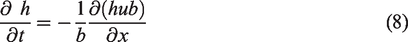
Based on the conservation of mass and momentum, the Saint-Venant system of the conventional SWE can be written as12,13

Here,
Here, modified SWEs are developed for the Venturi contraction and expansion for a rectangular channel. The centered TVD scheme is used for solving the modified SWE. MATLAB R2017a was used for the 1D simulations. The experiments were carried out in a trapezoidal open Venturi channel. The developed model is validated through experimental results without using analytical results. The paper proceeds from conventional SWE (“Modified 1-D SWEs for open Venturi channel” section) to the model development of modified SWE (“Centered TVD method for the modified 1D SWEs”) and the implementation of the TVD scheme for the modified SWE. The modified equations are then compared to the conventional SWE and validated with experimental results.
Modified 1D SWEs for open Venturi channel
A rectangular open Venturi channel is used for model development. The principle sketch is shown in Figure 1. The channel has a continuous bottom topography. In the Venturi section, the bottom width of the channel varies in the
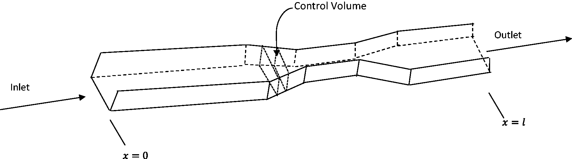
Principle sketch of the open Venturi channel with a rectangular cross-section. The selected control volume is in the Venturi contraction region. The top surface is open to the atmosphere.
Model development
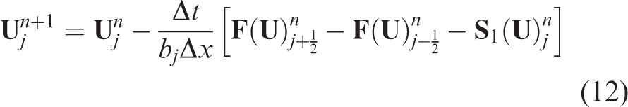
Figure 2 shows a spatial and time discretized grid for one time step, which is based on the finite volume method.
14
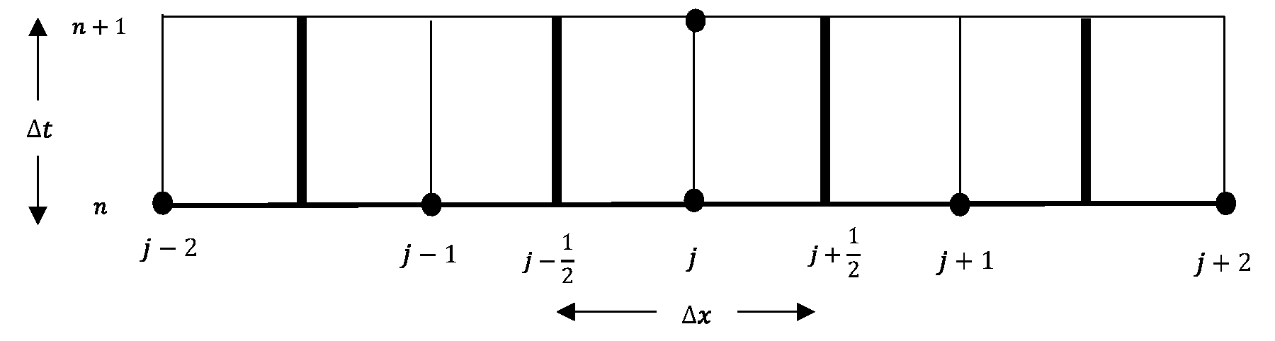
Semidiscretized grid, spatial discretization presented with
The model emphasizes the impact of contraction and expansion walls. The control volume is in the Venturi contraction region to consider a maximum number of boundaries. Figure 3 shows the forces acting on the control volume in the
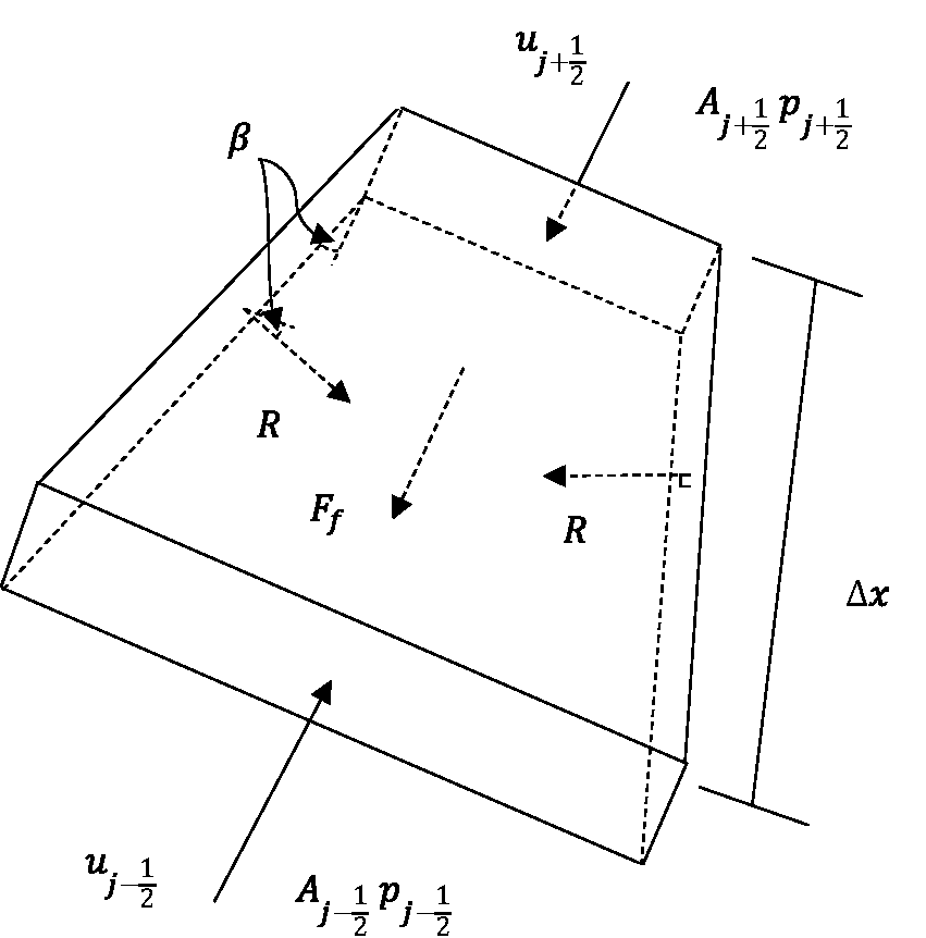
Forces on the control volume in the
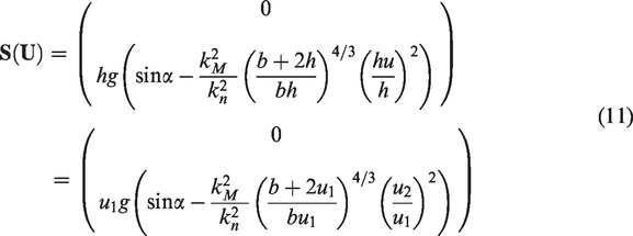
Fundamental conservation laws are used for model development; the temperature is assumed to be constant at room temperature, and density is also assumed to be constant. Two conservation equations are produced by applying mass and momentum balances to the control volume. There is no difference in the mass balance equation compared to the conventional SWE, which is equal to equation (1). Applying the momentum balance to the control volume
Here,
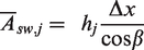
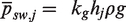
The pressure applied to the cross-section is a sum of atmospheric pressure and hydrostatic pressure. Atmospheric pressure is balanced from both sides of the cell faces as well as the top and bottom surfaces. The resultant hydrostatic pressure–force coming from the adjacent control volumes is
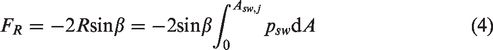
Here,

The central differencing approach for the flow depth of a channel with a rectangular cross-section,

When the channel has an inclined plane, a gravitational force acts with or against the flow direction.
Here,
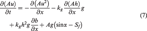
Compared to the conventional shallow water momentum balance equation, equation (2), the expression
Free falling at the end of the channel
In the experimental setup, the channel end was open, and the water was unhindered in flowing out of the channel. Accordingly, in the simulation, the physics of the last cells at the channel end needed to be modified with free falling properties. There is no friction effect when water does not touch the walls. Therefore,
Centered TVD method for the modified 1D SWEs
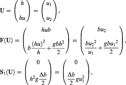
The conservation equations are based on a rectangular open Venturi channel. The bottom width
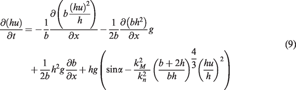
In equation (9),

Here
Here,
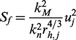
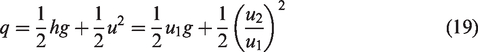
The source term is solved as

Here,

Here,
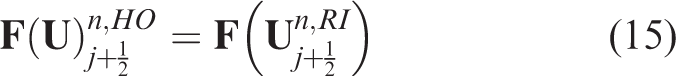

The low-order flux is based on the FORCE scheme
7

The Lax–Friedrichs (

The SUPER-BEE flux limiter (
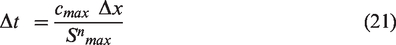
Time step is related to wave propagation speed.

According to the observations, Courant numbers higher than 0.7 led to high numerical diffusions at
Modified versus conventional SWEs for open Venturi channels
To compare the advantages of the modified SWE over conventional SWE, measurements and data from the experimental setup are used to supply the necessary variables. The results validate the modification. In the next section, the calculated results will further be compared to the measured results of the experiment as well as to the modeled results of 3D computational fluid dynamics (CFD). A more detailed description of the experimental setup will be given in section 6; here we only consider the values necessary for the calculations.
The total length of the channel is 3.7 m. The Venturi contraction region is


At initial conditions, the whole channel was filled with water, and all the node points were measuring the same flow depth and zero velocity. According to this condition, there was no flux propagation. However, in the contraction and expansion regions, the conventional SWE produced a flux difference, because of
Figure 4 shows a comparison between conventional SWE and modified SWE results after 0.01 s. The initial flow depth was 100 mm in the whole channel with zero velocity. At the contraction and expansion regions, flow depths and velocities change considerably in the conventional SWE. Moreover, these variations expand with time and extend into the whole channel. This error produces inaccurate results.
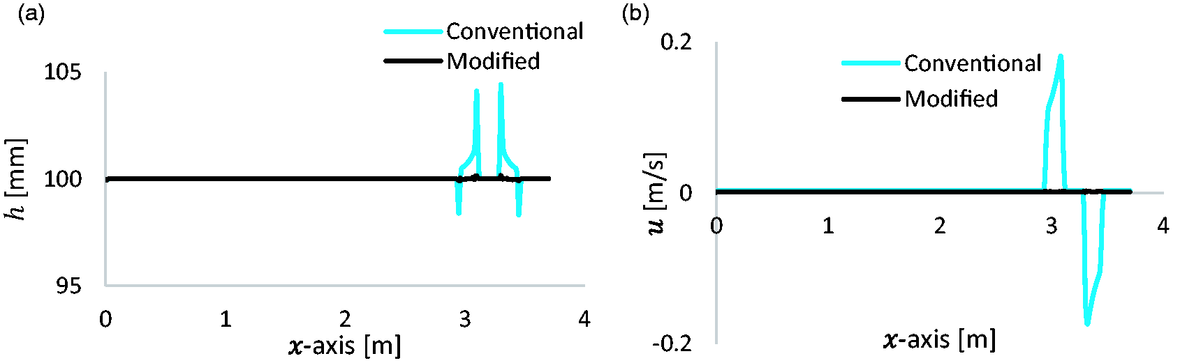
Comparison between conventional and modified SWE with zero velocity and constant flow depth in the whole channel at initial conditions. Results after 0.01 s: (a) flow depth along the
Model validation
The calculated results for the modified SWE are further validated by experimental and 3D CFD results.
Model validation with experimental results
The open Venturi channel used for the experimental model validation was located at University College of Southeast Norway. Level transmitters were located along the central axis of the channel. The transmitters were movable along the axis. The accuracy of the Rosemount ultrasonic 3107 level transmitters was ±2.5 mm for a measured distance of less than 1 m.
10
The channel had a trapezoidal shape with a trapezoidal angle of
From the inlet, water was added to the channel at the horizontal plane (
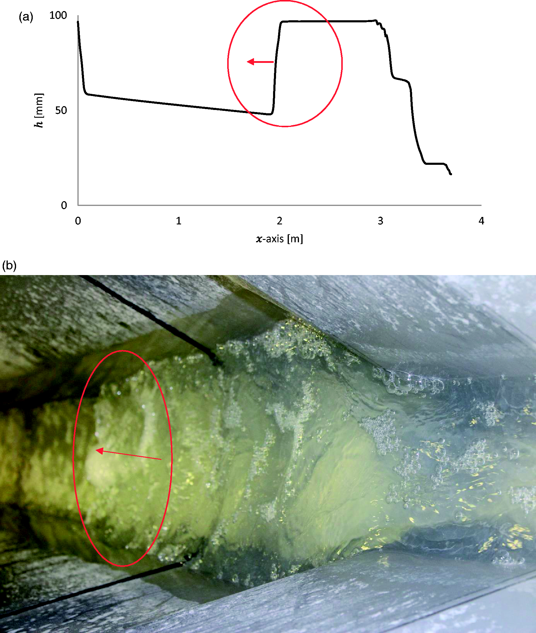
The hydraulic jump is moving upstream due to the wall-reflection pressure–force effect coming from the Venturi contraction walls, a dynamic result after 8.9 s. The arrows show the traveling direction of the hydraulic jump. The flow direction is opposite to the direction of the arrow. (a) The simulated flow depth result along the central axis and (b) the experimental results.
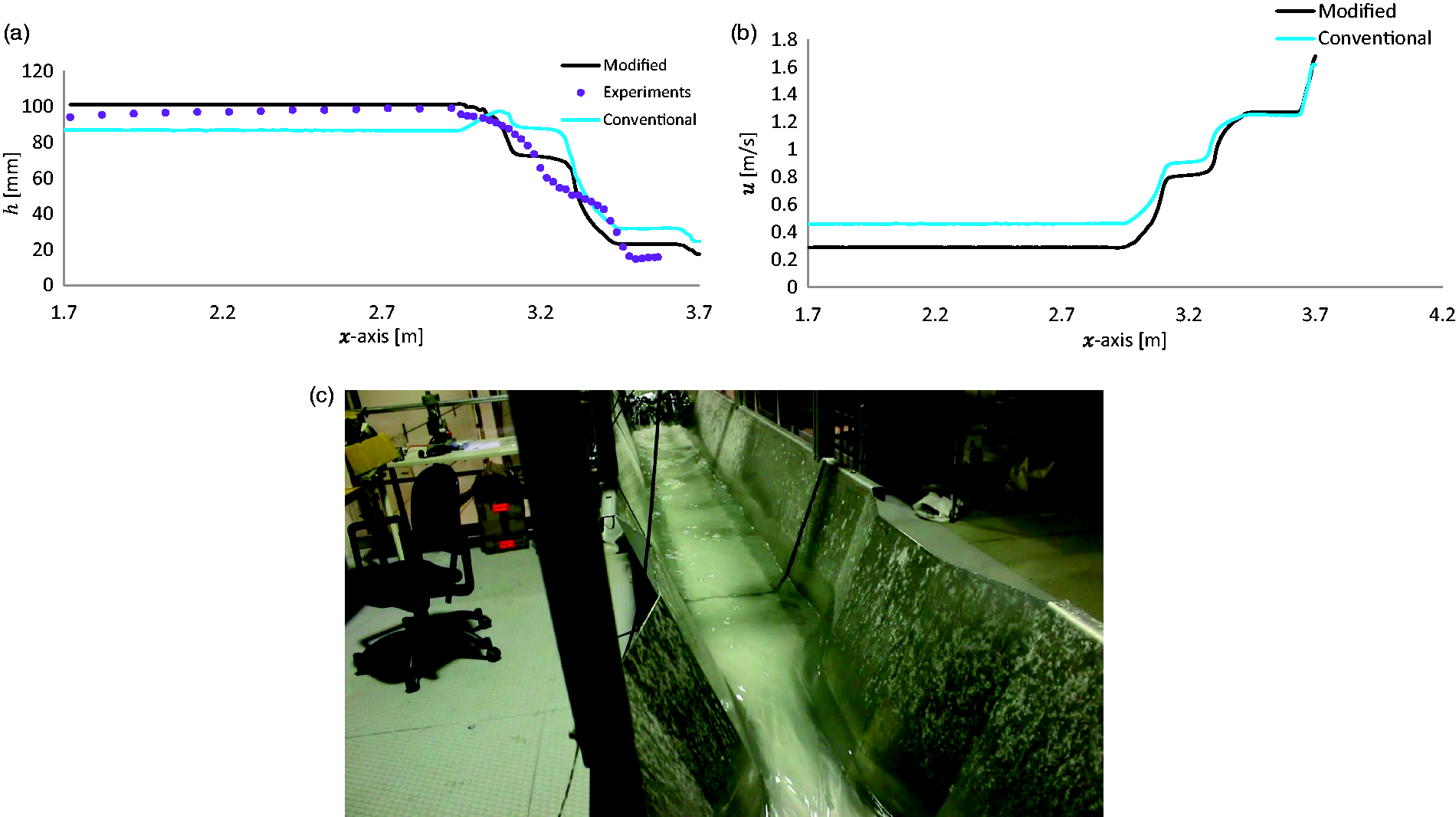
Quasi-steady state results, flow rate at 400 kg/min; (a) The simulated flow depth results along the central axis, (b) the simulated velocity results along the central axis, and (c) the experimental result.
Figure 6 shows the quasi-steady state results, following Figure 5. The flow depth comparison between the simulated and the experimental results in Figure 6(a) indicates the accuracy of the modified SWE. The modified SWE result is well matched with the experimental results compared to the conventional SWE. The channel at the horizontal plane, the Venturi contraction can cause a significant change in the flow regime. According to the flux calculation in the contraction and the expansion regions, the results from the conventional SWE deviated from the experimental results at quasi-steady state. The wall-reflection pressure–force coming from the contraction walls changed the flow regime from supercritical to subcritical, whole channel section before the contraction region. The velocity profile in Figure 6(b) can be used to explain the wall-reflection pressure–force effect in the Venturi expansion region. At the expansion region (
Model validation with 3D CFD result
Further, the result of the modified SWE result was compared to a CFD result. 16 Three-dimensional CFD simulations are based on the volume of fluid method. Water and air are the materials in the fluid domain. An artificial compression term is activated at the interface.17–19 Time discretization is based on the implicit Euler method for a transient calculation. Pressure–velocity coupling is based on the SIMPLE scheme with a second-order upwind correction. The standard k–ε model is used for the turbulence handling. Wall surface roughness is used to calculate the wall friction, which is 15 µm. The mesh contains 0.74 million elements with a maximum cell size of 10 mm. ANSYS Fluent 16.2 (commercial code) was used as the simulation tool.10,16 The 3D CFD study was done with the same experimental setup for 100 kg/min flow rate. The quasi-steady state results are shown in Figure 7. The modified SWE result was well matched with the CFD result compared to the conventional SWE. A similar flow profile was achieved by Berg et al. 20 from CFD simulation for an open Venturi channel. The error propagated in the contraction and expansion regions caused the high deviation when using the conventional SWE.
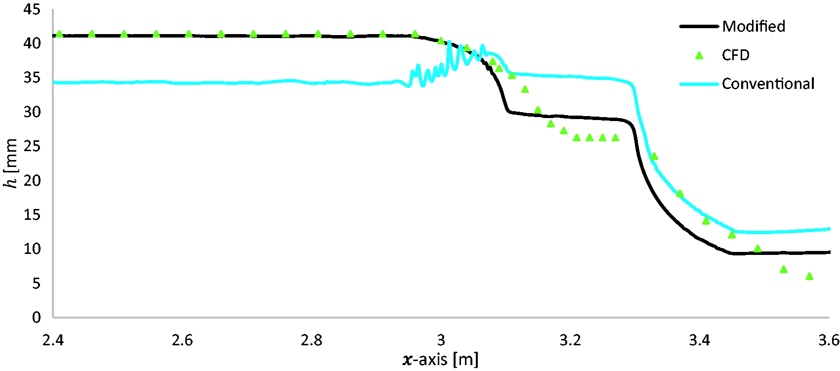
A comparison with 3D CFD result with the modified and the conventional shallow water results, quasi-steady state, the flow rate at 100 kg/min. The CFD result is from Welahettige et al. 16 CFD: computational fluid dynamics.
Figure 8 shows a flow surface for the full channel (iso-surface of water volume fraction of 0.5) from the 3D CFD simulations, 10 which is related to Figure 6(a). The flow rate is 400 kg/min, and the channel is at a horizontal angle. One-dimensional simulation surface profile is well matched with the 3D CFD surface profile.
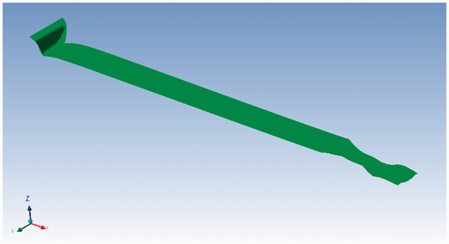
Water flow rate 400 kg/min and open channel at horizontal position: Simulated flow surface for the full channel (iso-surface of water volume fraction of 0.5). The flow direction is left to right. 10
Conclusion and future work
The 1D conventional SWEs cannot be applied to a channel with a contraction and an expansion region (Venturi channel). Because conventional SWE neglect the wall-reflection pressure–force effect, they are suitable for prismatic channels only. The modified 1D SWEs are developed by considering the wall-reflection pressure–force effect. The modified SWEs can be applied to both prismatic and nonprismatic channels, especially those with contraction and the expansion regions.
This study will further extend into drilling fluid flow measurement in an open Venturi channel. The non-Newtonian properties of drilling fluid will be considered. Further, the scenario of a reflection hydraulic jump hitting the inlet will be considered in the future study.
Footnotes
Acknowledgment
The authors gratefully acknowledge the resources for experiments and simulations provided by the University College of Southeast Norway.
Declaration of conflicting interests
The author(s) declared no potential conflicts of interest with respect to the research, authorship, and/or publication of this article.
Funding
The author(s) disclosed receipt of the following financial support for the research, authorship, and/or publication of this article: Economic support from The Research Council of Norway and Statoil ASA through project no. 255348/E30 “Sensors and models for improved kick/loss detection in drilling (Semi-kidd)” is gratefully acknowledged.