Flow regime changes at hydraulic jumps in an open Venturi channel for Newtonian fluid

Abstract

The aim of this paper is to study flow regime changes of Newtonian fluid flow in an open Venturi channel. The simulations are based on the volume of fluid method with interface tracking. ANSYS Fluent 16.2 (commercial code) is used as the simulation tool. The simulation results are validated with experimental results. The experiments were conducted in an open Venturi channel with water at atmospheric condition. The inlet water flow rate was 400 kg/min. The flow depth was measured by using ultrasonic level sensors. Both experiment and simulation were done for the channel inclination angles 0°, −0.7°, and −1.5°. The agreement between computed and experimental results is satisfactory. At horizontal condition, flow in the channel is supercritical until contraction and subcritical after the contraction. There is a hydraulic jump separating the supercritical and subcritical flow. The position of the hydraulic jump oscillates within a region of about 100 mm. Hydraulic jumps coming from the contraction walls to the upstream flow are the main reasons for the conversion of supercritical flow into subcritical flow. An “oblique jump” can be seen where there is a supercritical flow in the contraction. There is a triple point in this oblique jump: the triple point consists of two hydraulic jumps coming from the contraction walls and the resultant wave. The highest flow depth and the lowest velocity in the triple point are found at the oblique jump.

Introduction

Drill bit pressure control (Kick/Loss detection) is a critical task in oil well drilling. Drill mud flow control is one method to control the pressure at the drill bit. Coriolis flow meters are currently used for mud flow measurements. However, since these flow meters are expensive, open Venturi channel mud flow measurement could be a cost-effective alternative. It is thus of interest to understand the flow behavior in an open Venturi channel.

Molls and Hanif Chaudhry ¹ have developed a model to solve unsteady depth-averaged equations and it was tested in a contraction channel in a computational study. Berg et al. ² have done a feasibility study about the possibility of flow rate measurements in a Venturi flume. They recognized that the occurrence of a “level jump” depends on fluid properties, length of the flume, and computational time. Datta and Debnath ³ used the volume of fluid (VOF) model for an open channel with different contraction ratios. They observed that turbulence intensity increases as the contraction ratio decreases. Patel and Gill ⁴ used the VOF model for the curved open channel flow in computational fluid dynamics (CFD) simulation. Agu et al. ⁵ developed a numerical scheme to predict the transcritical flow in a Venturi channel using the Saint-Venant equations. When the supercritical flow regime passes through the critical flow regime into the subcritical flow regime, the hydraulic jump is propagated due to the energy losses.^6,7 Yen ⁸ studied open channel flow resistance. Benjamin and Onno ⁹ studied shallow water flow through a channel contraction. Wierschem and Aksel ¹⁰ studied hydraulic jumps and standing waves in a gravity-driven flow of viscous liquid in an open channel. Hänsch et al. ¹¹ introduced a multifluid two-fluid concept combining a dispersed and a continuous gas phase in one computational domain that could be used to describe bubble behavior in a hydraulic jump. The VOF model can be used for the open channel flow.^12,13

This study is the beginning of our future study for the development of a model for non-Newtonian fluid drill cutting flow control. The main objective of this study is to identify the flow regime changes of Newtonian fluid in an open Venturi channel. The simulation results are validated with experimental results.

CFD models

The fluid domain contains water and air. The interface is changing (water level changing) along the Venturi channel. The VOF method with surface tracking is applied to a fixed Eulerian mesh. The free surface between flowing fluid (water) and fluid above (air) is important for flow depth measurement. Water is considered as the secondary phase in these simulations (air might also be used as the secondary phase). Water volume fraction ${\alpha }_2$ of the cells is contained by

$$0<{\alpha }_2<1$$

(1)

By assuming isothermal, incompressible, and immiscible conditions, the mass balance equation can be given as

$$\frac{\partial {\alpha }_2}{\partial t}=-\mathit{div}({\alpha }_2\overrightarrow{U})$$

(2)

At the interface, an artificial compression term is activated. Therefore, equation (2) can be converted into^14–16

$$\frac{\partial {\alpha }_2}{\partial t}=-\mathit{div}({\alpha }_2\overrightarrow{U})-\mathit{div}({\alpha }_2(1-{\alpha }_2){\overrightarrow{U}}_r)$$

(3)

${\alpha }_2(1-{\alpha }_2)$ is only active at the interface, since it will disappear when ${\alpha }_2=0$ or ${\alpha }_2=1$ . Here, $\overrightarrow{U}$ is the three-dimensional velocity component, ${\overrightarrow{U}}_r$ is the velocity field suitable to compress the interface. The maximum velocity at the transition region is an approximation for ${\overrightarrow{U}}_r$ . The compression is considered perpendicular to the interface.

Time discretization is based on the implicit Euler method. Pressure–velocity coupling is based on the Semi Implicit Method for Pressure Linked Equations scheme with a second-order upwind correction. The standard k−ɛ model is used for turbulence handling.

x momentum

$$\frac{\partial \rho u}{\partial t}+\mathit{div}(\rho u\overrightarrow{U})=-\frac{\partial p}{\partial x}+\mathit{div}(\mu \mathit{grad}(u))+F_{\mathit{sx}}$$

(4)

y momentum

$$\frac{\partial \rho v}{\partial t}+\mathit{div}(\rho v\overrightarrow{U})=-\frac{\partial p}{\partial y}+\mathit{div}(\mu \mathit{grad}(v))+F_{\mathit{sy}}$$

(5)

z momentum

$$\frac{\partial \rho w}{\partial t}+\mathit{div}(\rho w\overrightarrow{U})=-\frac{\partial p}{\partial z}+\mathit{div}(\mu \mathit{grad}(w))+F_{\mathit{sz}}+\rho g$$

(6)

Here $u,v$ , and w are the velocity components in the $x,y$ , and z directions, respectively. g is the acceleration of gravity. ${\overrightarrow{F}}_s$ is the surface tension force; it is active only at the free surface

$${\overrightarrow{F}}_s=\sigma k\overrightarrow{n}$$

(7)

$$\overrightarrow{n}=\frac{\mathit{grad}(\alpha )}{|\mathit{grad}(\alpha )|}$$

(8)

$$k=\mathit{div}(\overrightarrow{n})$$

(9)

Here σ is the surface tension coefficient,k is the curvature of the interface, and $\overrightarrow{n}$ is the normal vector to interface. The material properties, density ρ and viscosity μ, are considered as

$$\rho ={\alpha }_2{\rho }_2+(1-{\alpha }_2){\rho }_1$$

(10)

$$\mu ={\alpha }_2{\mu }_2+(1-{\alpha }_2){\mu }_1$$

(11)

${\rho }_1$ and ${\rho }_2$ are the densities of air and water. ${\mu }_1$ and ${\mu }_2$ are the viscosities of air and water. Wall surface roughness is commonly characterized by the normalized roughness height $K_s^{+}$ ^6,12,17

$$K_s^{+}=\frac{\rho K_s{u}^{*}}{\mu }$$

(12)

Here K_s is the physical roughness height, while

$$u^{*}=C_{\mu }^{1/4}{\kappa }^{1/2}$$

(13)

Here $C_{\mu }=0.09$ is a k−ɛ model constant and $\kappa =0.4$ is the von Karman’s constant. According to these conditions, there are three main flow regimes:

If $K_s^{+}\le 2.25$ , the system is hydrodynamically smooth,

If $2.25<K_s^{+}\le 90$ , the system is transitional,

If $90<K_s^{+}$ the system is fully rough.

The calculated $K_s^{+}$ value for this case is approximately 5.2. Therefore, transitional wall roughness is active. This calculation is based on the stainless steel physical roughness height.

Critical depth calculation

The dimensionless Froude number ( $\text{Fr}$ ) is used for the characterization of the open-channel flows, which is defined as the ratio of the inertia force and hydrostatic force^6,12

$$\text{Fr}=\frac{\overline{U}}{\sqrt{\mathit{gl}}}$$

(14)

Here $\overline{U}$ is the velocity magnitude of the fluid and l is the characteristic length. There can be a wave propagation based on the velocity magnitude and the distance from bottom surface to the free surface level. The wave speed is given as

$${\overline{U}}_{\mathit{wave}}=\overline{U}\pm \sqrt{\mathit{gl}}$$

(15)

Three types of waves can be categorized based on the $\text{Fr}$ number value.

Case 1

If $\text{Fr}$  < 1, then $\overline{U}$  <  $\sqrt{\mathit{gl}}$ , therefore ${\overline{U}}_{\mathit{wave}}$  < 0 or ${\overline{U}}_{\mathit{wave}}$  > 0. This is called subcritical flow. The wave disturbance can travel upstream as well as downstream. In this case, the downstream flow condition may affect the upstream flow. Here, $l>l_c$ .

Case 2

If $\text{Fr}=1$ , then $\overline{U}=\sqrt{{\mathit{gl}}_c}$ , therefore ${\overline{U}}_{\mathit{wave}}=0$ . This is called critical flow. The propagated wave disturbance remains and it will not affect either upstream or downstream. Here, $l=l_c$ .

Case 3

If $\text{Fr}$  > 1, then $\overline{U}$  >  $\sqrt{\mathit{gl}}$ , therefore ${\overline{U}}_{\mathit{wave}}$  > 0. This is called supercritical flow. The disturbances cannot travel upstream. Rapid flows are prominent for supercritical flow. Here, $l<l_c$ .

Critical flow depth h_c is important in order to identify whether the flow condition is supercritical or subcritical. Figure 1 shows the sketch of a cross sectional view of the trapezoidal channel. Here b is the bottom depth, h_c is the critical flow depth, and θ is the trapezoidal angle.

Figure 1.

Cross sectional sketch of the trapezoidal open channel with critical flow depth.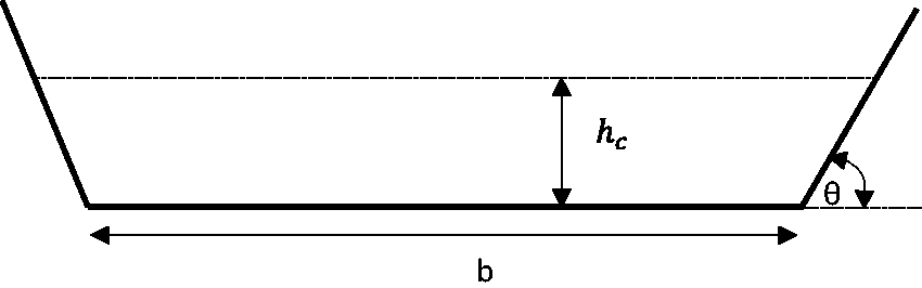

At critical flow condition

$$\overline{U}=\sqrt{{\mathit{gl}}_c}$$

(16)

The flow rate (Q) can be defined as

$$\text{d}Q=U\text{d}A$$

(17)

The area (A) perpendicular to flow direction is given as

$$A=(b+\frac{h_c}{\text{tan}\theta })h_c$$

(18)

The ratio between area and free surface width gives the characteristic length for the trapezoidal. At critical flow

$$l_c=\frac{A}{b+\frac{2h_c}{\text{tan}\theta }}$$

(19)

By substituting equations (17) to (19) for equation (16), a critical depth equation can be derived as

$$g(b+\frac{h_c}{\text{tan}\theta }{)}^3{h}_c^3-Q^2(b+\frac{2h_c}{\text{tan}\theta })=0$$

(20)

In this study, the bottom width (b) is the only variable, with the critical depth and other parameters as constants along the x-axis. θ is equal to 70°. The total length of the channel is 3.7 m and the measurement start from the inlet of the channel (see Figure 2).

Figure 2.

Three-dimensional geometry of a trapezoidal channel with a Venturi region; x = 0 m is the inlet of the channel. Contraction starts at x = 2.95 m and ends at 3.45 m. The bottom width is 0.2 m for 0 m < x < 2.95 m and 3.45 m < x < 3.7 m. The bottom width is 0.1 m for 3.1 m < x < 3.3 m. The trapezoidal angle is 70°. The bottom surface has a constant slope (flat).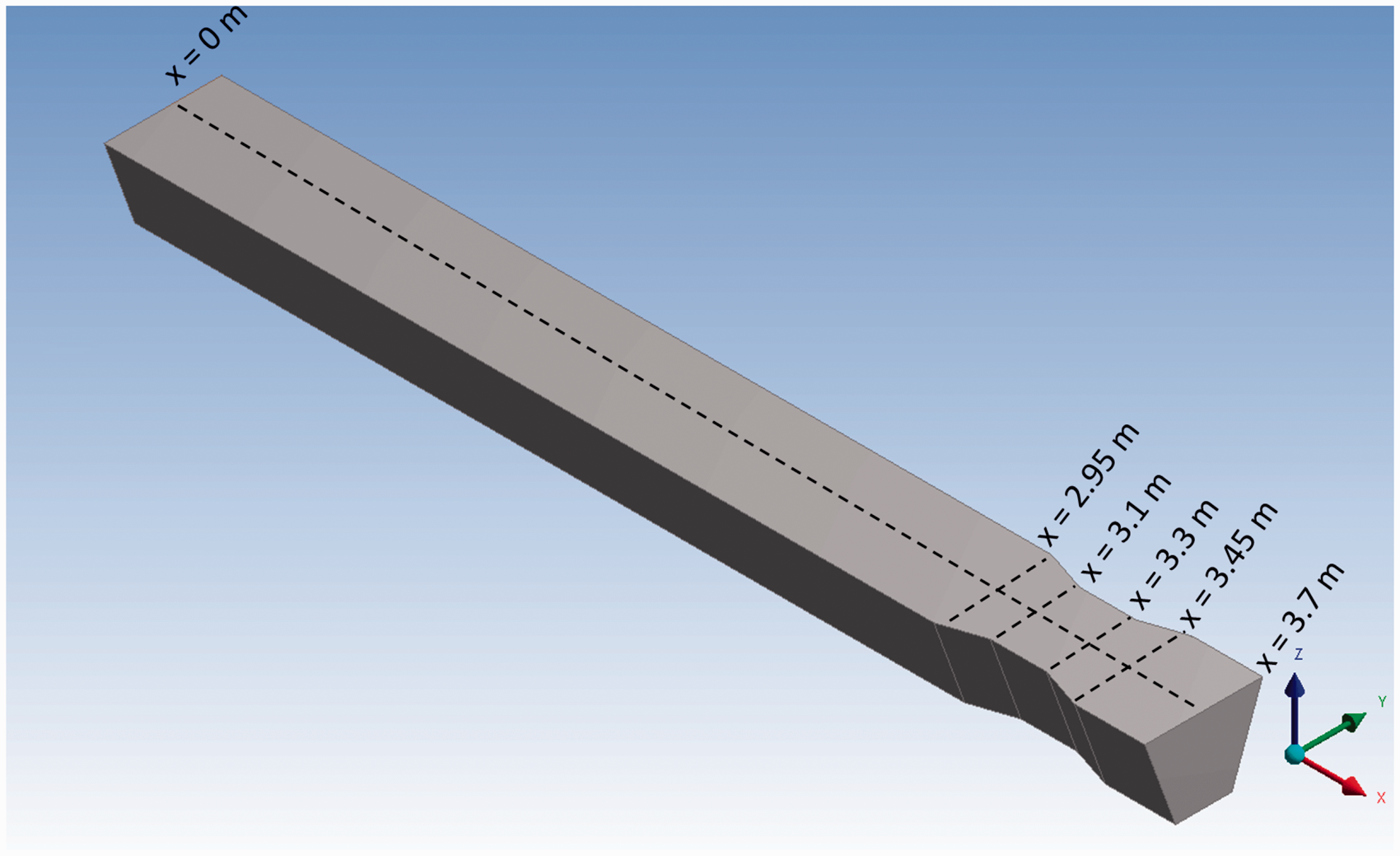

In this case, the bottom width can be defined as a function of x:

For $x=0\text{m}\hspace{1em}\text{to}\hspace{1em}2.95\text{m}:b=0.2\text{m}$

For $x=2.95\text{m}\hspace{1em}\text{to}\hspace{1em}3.1\text{m}:b=0.2-\frac{x-2.95}{1.5}$

For $x=3.1\text{m}\hspace{1em}\text{to}\hspace{1em}3.3\text{m}:b=0.1\text{m}$

For $x=3.3\text{m}\hspace{1em}\text{to}\hspace{1em}3.45\text{m}:b=0.1+\frac{x-3.3}{1.5}$

For $x=3.45\text{m}\hspace{1em}\text{to}\hspace{1em}3.7\text{m}:b=0.2\text{m}$

The calculated critical depth for the Venturi channel is shown in Figures 5, 7 and 10. Akan’s ¹⁸ calculations are matching with these calculations.

Geometry, mesh, and boundary conditions

Geometry and mesh

A 3D geometry is shown in Figure 2, which is used in the simulations. The dimensions of the geometry match with the open channel experimental setup. ANSYS Fluent DesignModeler and ANSYS Meshing tools are used for drawing the geometry and generating the mesh, respectively. There is a large distance between the inlet and the start of the contraction. This is to achieve more stable flow conditions before the Venturi contraction in order to reduce upstream disturbances at the Venturi.

The mesh that is used in the simulation contains 0.74 million elements with a maximum cell size of 10 mm. Inflation layers are added near the wall boundaries for better prediction.

Boundary conditions

The upstream boundary condition was defined as “mass flow inlet” for each phase. The inlet water flow rate was 400 kg/min and air inlet flow rate is equal to zero. The outlet was considered a “pressure outlet.” The top boundary, which was open to the atmosphere, was defined as a “pressure outlet” at “open channel” conditions. “Bottom level” was defined at z = 0 m. All solid walls were considered as “wall.” These walls are stationary walls and no-slip condition applies. The wall roughness was matched with a stainless steel wall similar to experimental conditions. Roughness height is 15 µm for stainless steel. The roughness constant was set to 0.5. ³ The fluid domain initializes with only air at atmospheric condition. This means that water is added continuously to an empty channel (with air) at startup.

Experimental setup

The Venturi rig is located at University College of Southeast Norway (see Figure 3). The experimental results of this open Venturi channel are used for comparison with simulation results. The complete circuit of the rig contains a “mud” -mixing tank, a mud circulating pump, a Venturi channel, and a mud return tank. The sensing instruments in the setup are a Coriolis mass flow meter, pressure transmitters, temperature transmitters, and ultrasonic level transmitters. The level transmitters are located along the central axis of the channel and can be moved along the central axis. The accuracy of the Rosemount ultrasonic 3107 level transmitters is ±2.5 mm for a measured distance of less than 1 m. ¹⁹ The dimensions of the open channel are shown in Figure 2. All of the experimental values presented in this paper are average values of sensor readings taken over a period of 5 min in each location. The channel inclination can be changed; a negative channel inclination indicates a downward direction.

Figure 3.

Experimental setup: (a) Open channel with level sensors and (b) pump station.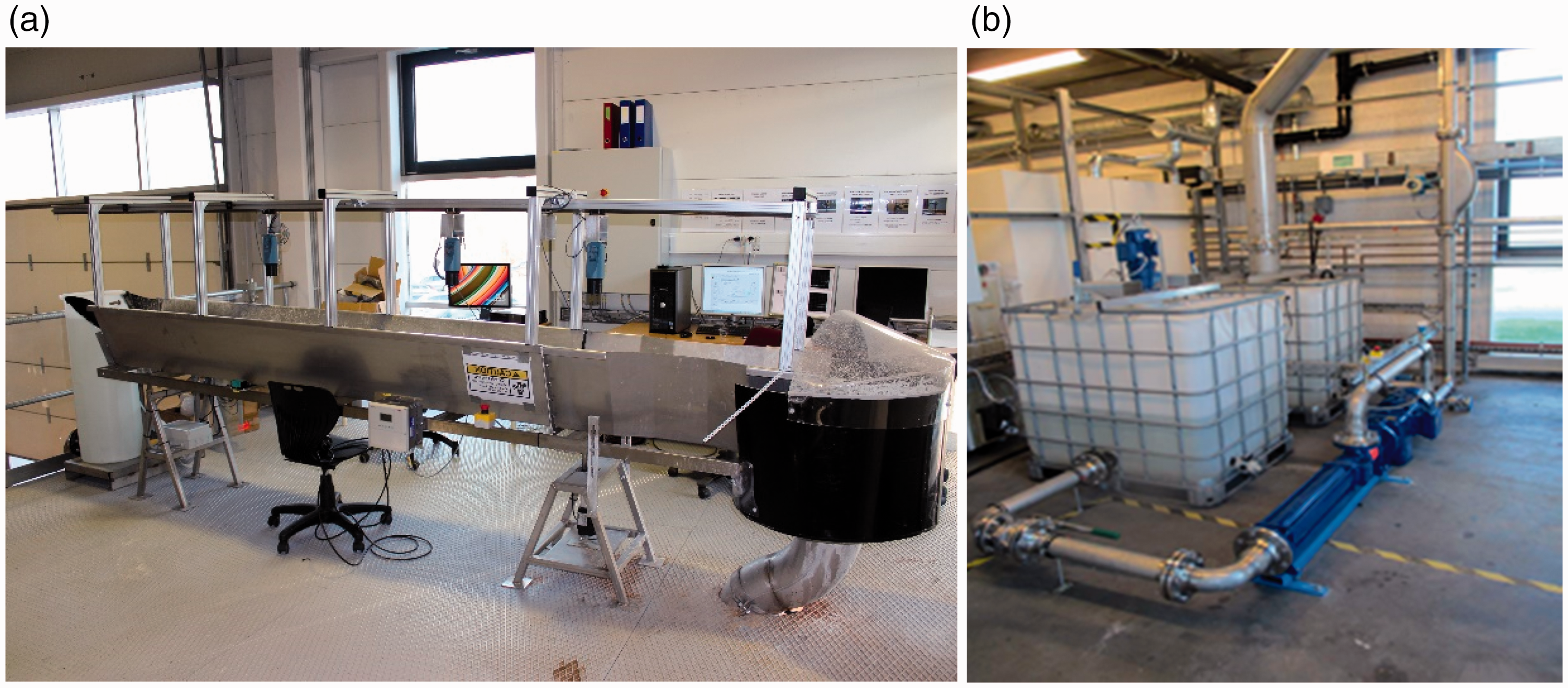

Results

Experiment and simulation were done with a water flow rate at 400 kg/min for different channel inclination angles: 0°, −0.7°, and −1.5°. The ensuing flow regime changes are observed in the evaluation of the results.

Subcritical flow to supercritical flow

In this case, water flow rate was set to 400 kg/min and the inclination angle was zero. This means that the channel was at horizontal condition. Figure 4 shows the experimental flow depth in the Venturi region and simulated water surface for the complete channel. The water surface is very stable before the contraction. Flow depth is reduced and flow velocity is increased after the Venturi contraction.

Figure 4.

Water flow rate 400 kg/min and open channel at horizontal position: (a) Experimental flow depth at the Venturi region, (b) simulated flow surface for full channel (iso-surface of water volume fraction of 0.5). The flow direction is left to right.

Figure 5.

Critical depth, experimental flow depth, and simulated flow depth for water flow rate at 400 kg/min and inclination angle 0° along the channel’s central axis (x-axis).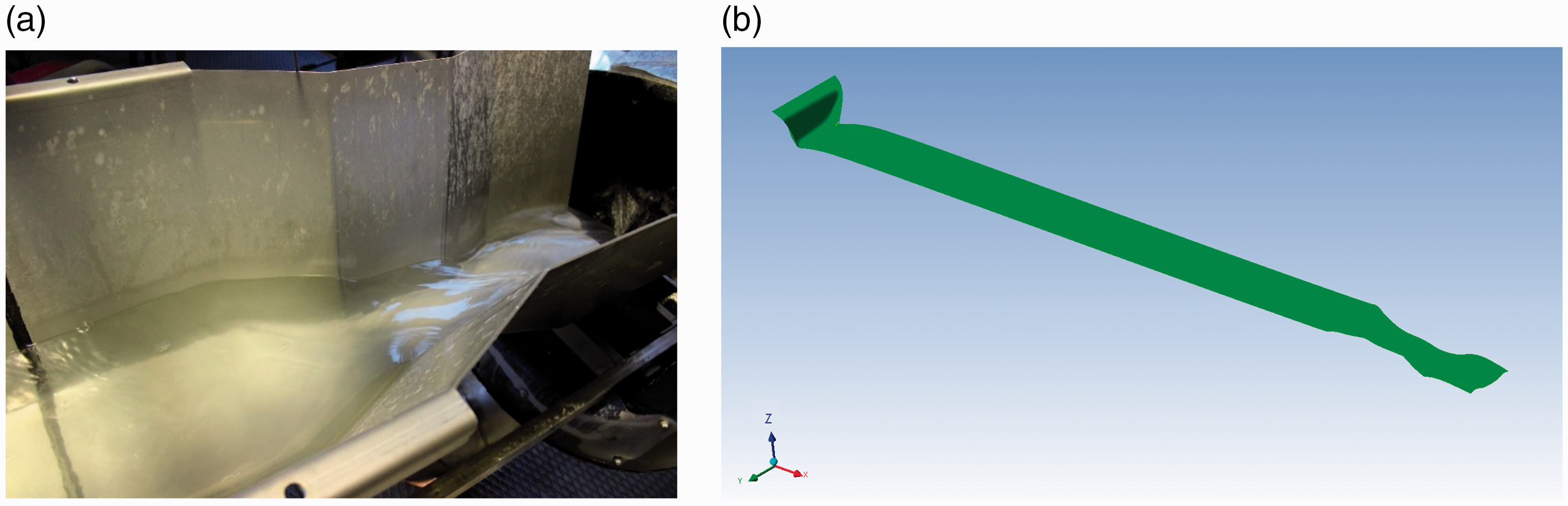

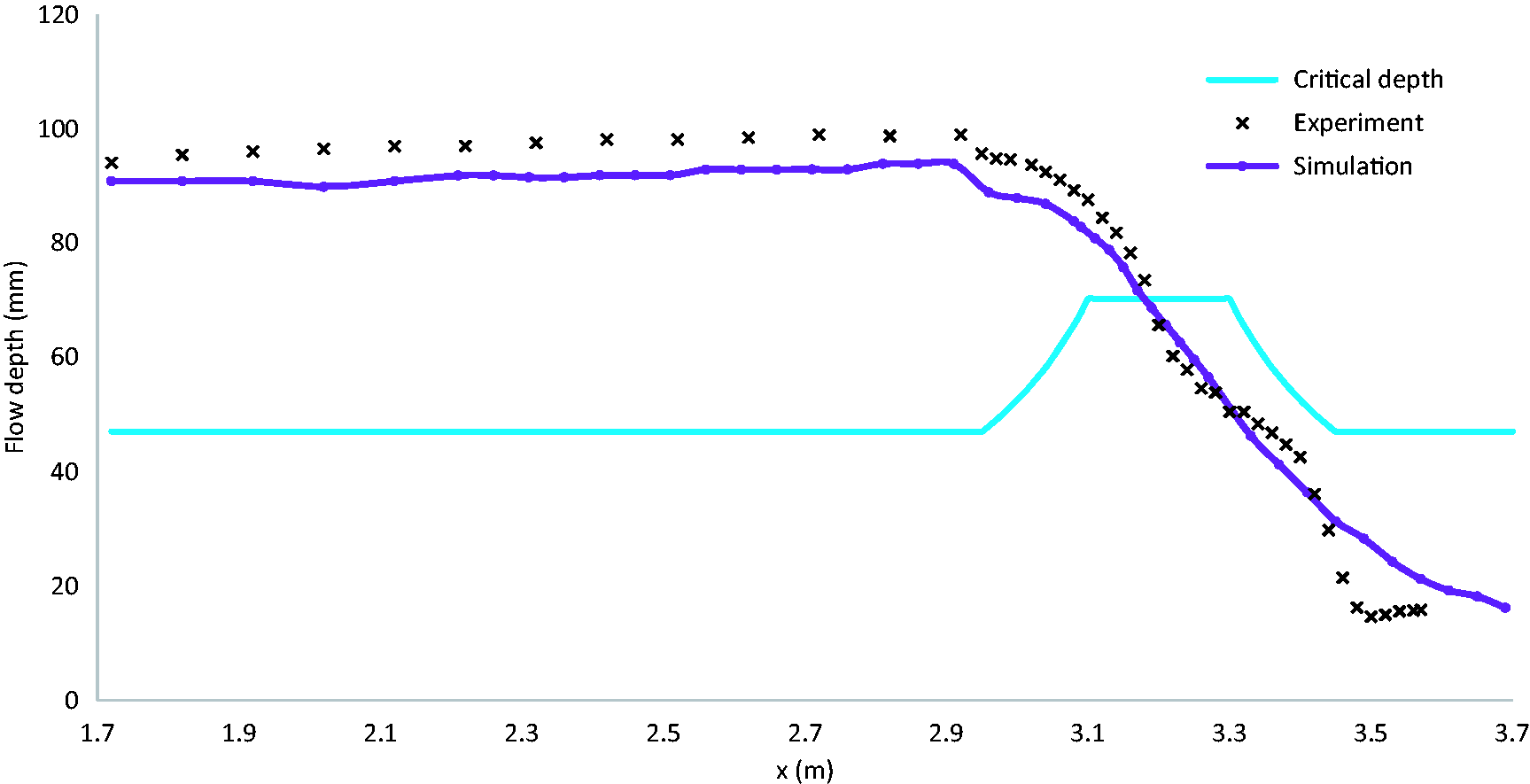
Figure 5 shows the flow depth along the centerline from x = 1.7 m to x = 3.7 m for both experiment and simulation. The calculated critical depth is important for identifying the flow regimes, whether they are subcritical or supercritical. The flow depth in range of 1.7 m < x < 3.18 m is subcritical because flow depth is higher than critical depth. Flow depth below critical depth (3.18 m < x < 3.7 m) shows supercritical flow behavior. Subcritical flow behavior is propagated due to the barriers of the contraction to the flow path. There is no barrier at the end of the channel and, therefore, no back wave propagation to the upstream flow. Because of this, the flow becomes supercritical at the end of the channel.

Supercritical flow to subcritical flow (hydraulic jump)

To generate a hydraulic jump before the contraction region, the channel inclination angle was changed to −0.7° in the downward direction. Because of this, gravity flow support ( $\text{gsin}0.7$ ) came in the x direction. The water flow rate was 400 kg/min. Figure 6 shows the hydraulic jump results of experimental and simulated iso-surface. This hydraulic jump was propagated before the contraction region (at x = 2.26 m). Flow depth was lower before the hydraulic jump and higher after the hydraulic jump. In the quasi steady state, the toe of the hydraulic jump oscillated backward and forward within approximately 100 mm. Air entrainment generated more bubbles at the hydraulic jump toe as seen in Figure 6(a) and described by Xiang et al. ²⁰

Figure 6.

Water flow rate 400 kg/min and the channel inclination −0.7° in downward direction: (a) Experimental flow depth before the contraction and (b) simulated flow surface for full channel (iso-surface of water volume fraction of 0.5). The flow direction is left to right.

Figure 7.

Critical depth, experimental flow depth, and simulated flow depth for water flow rate at 400 kg/min and inclination angle −0.7°.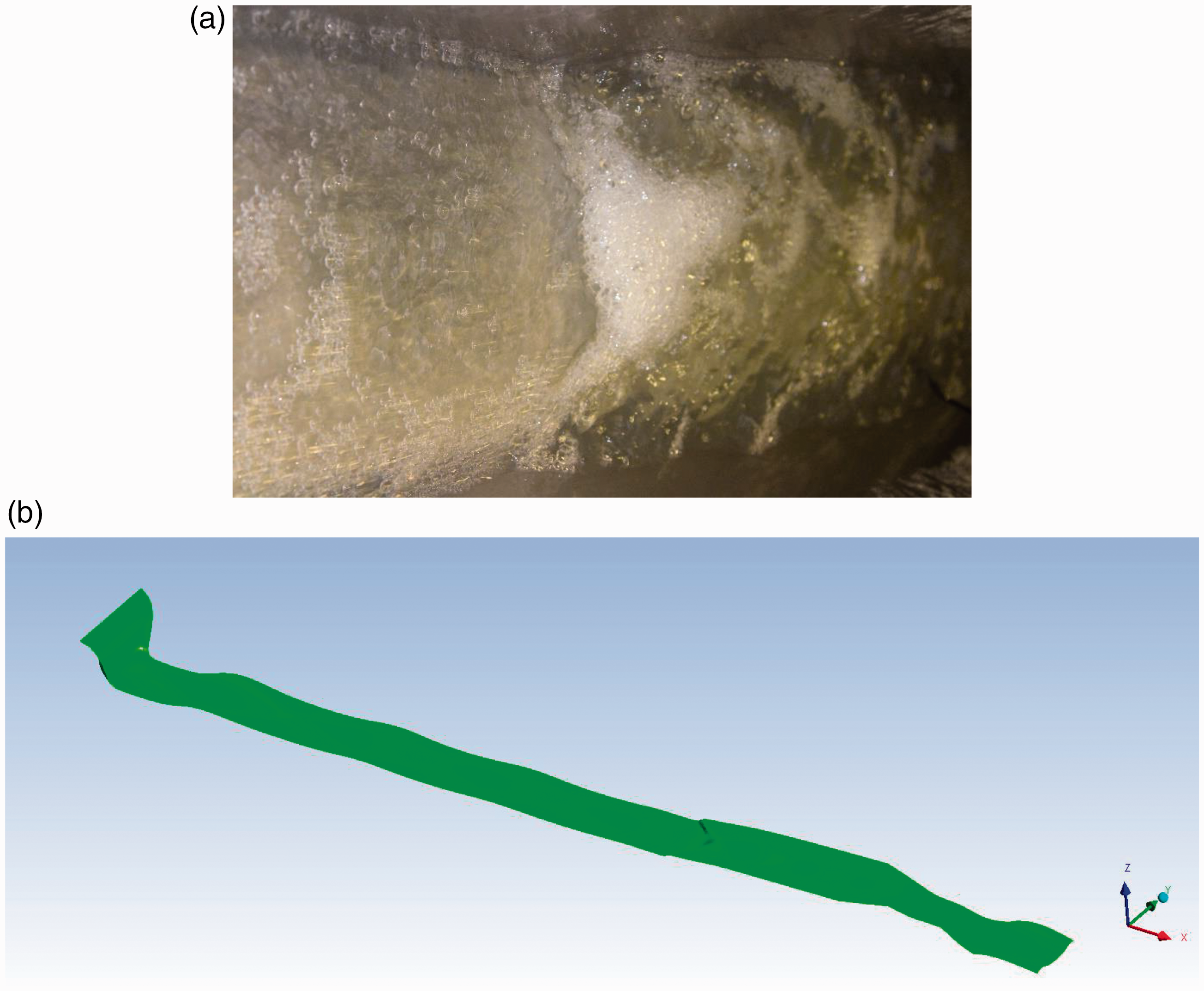

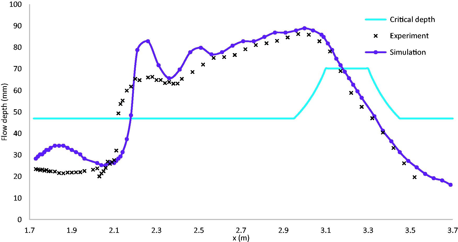
As shown in Figure 7, at x = 1.7 m to x = 2.17 flow depth was lower than critical depth and flow was supercritical. At x = 1.8 m to x = 3.17 m, flow depth was higher than critical depth and flow was subcritical. The hydraulic jump was propagated due to the conversion of supercritical flow into subcritical flow. Because of the unsteady hydraulic front in the region x = 1.7 m to x = 2.5 m, experimental results and simulated results are only approximately matched: the hydraulic jump front was moving forward and backward due to the hydraulic jumps coming from the contraction walls. This hydraulic jump was strong enough to convert supercritical flow into subcritical flow. Because of this, flow depth gradually increased up to x = 3.0 m. Flow depth started to decrease from x = 3.0 m to the outlet. This was due to no hydraulic jump propagation into the upstream, as explained above. Also in this case, flow depth became supercritical after x = 3.18 m. The water surface was very stable after x = 3.18 m. Therefore, simulation results almost exactly match the experimental results.

Supercritical flow at the Venturi (oblique jump)

In this case, the channel inclination angle was further increased to −1.5° in the downward direction. The flow rate was 400 kg/min. Flow velocity was very fast compared to the other cases. The average flow depth along the channel was almost flat up to the contraction region. However, there was a large “oblique jump” after the Venturi contraction, as shown in Figure 8. The simulated results show a similar oblique jump. The water level near the contraction wall increased due to a hydraulic jump coming from the walls. The oblique jump disappeared at the end of the Venturi due to channel expansion. When the channel expands, there is no strong hydraulic jump coming from the walls compared to channel contraction.

Figure 8.

Water flow rate 400 kg/min and channel inclination −1.5° in downward direction: (a) Experimental flow depth before the contraction and (b) simulated flow surface for full channel (iso-surface of water volume fraction of 0.5). Flow direction is left to right.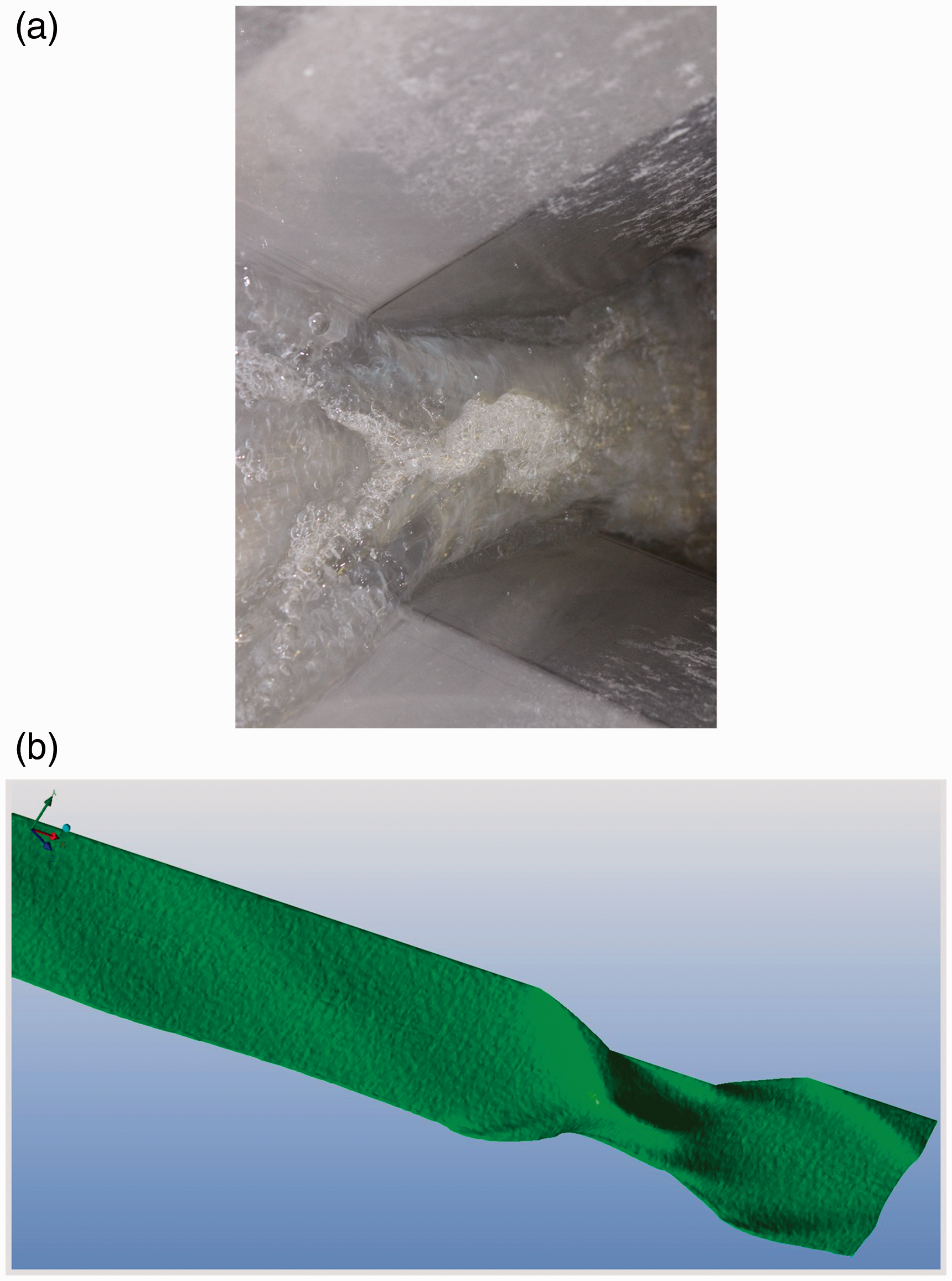

The Rosemount Ultrasonic 3107 Level Transmitter used for measurement has a 6° beam half angle. ¹⁹ It measures the average flow depth in its projecting area. The width of the oblique jump is small, as shown in Figure 9. Therefore, the level sensors only measure average values of the flow depth and do not provide a separate measurement of the highest value of flow depth.

Figure 9.

The cross sectional view of the oblique jump. Water volume fraction at x = 3.19 m.

Figure 10.

Oblique jump: Critical depth, experimental flow depth, and simulated flow depth for water flow rate at 400 kg/min and inclination angle −1.5°.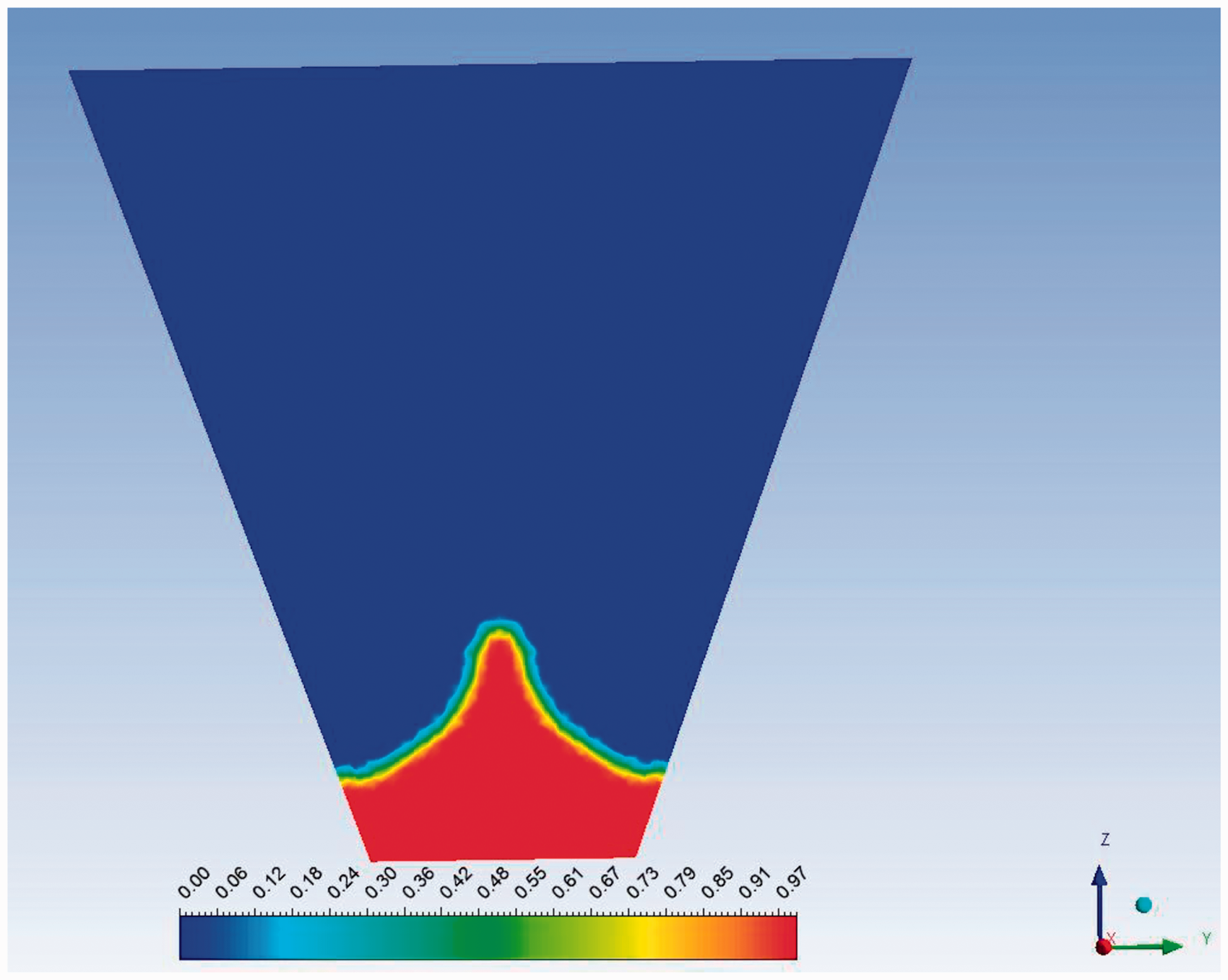

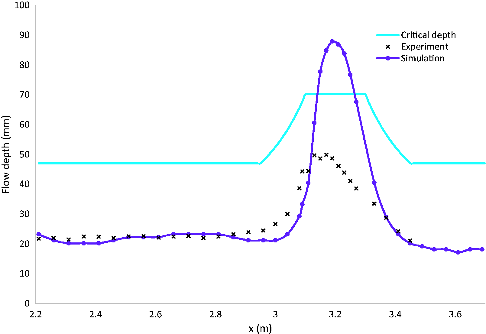
The “oblique jump” starts at the end of the contraction of Venturi and ends with the start of the expansion of the Venturi (x = 3.1 m to x = 3.3 m) as shown in Figure 10. The simulated flow depth reaches a maximum of up to 87 mm. The experimental values show smaller values compared to the simulation due to flow depth averaging as explained previously. The average flow depth is supercritical in the whole channel because it is smaller than critical depth. The oblique jumps are strongly visible at supercritical flow.

Discussion

Hydraulic jumps coming from the contraction walls are stronger than the upstream flow, when the system is completely subcritical before the Venturi contraction. Figure 11 shows the hydraulic jump coming from the contraction walls to the upstream flow in transient condition. We assume at the beginning that there is no water inside the channel. As water is added into the channel, it will hit the contraction walls and propagate a hydraulic jump. The strength of the hydraulic jump is determined by the channel inclination angle and flow rate. The downward angle gives a gravitational support to increase the flow velocity. For a hydraulic jump to occur in the middle of the channel, the upstream force (friction balancing force coming with upstream fluid) needs to be strong enough to neutralize the hydraulic jump coming to the upstream. The position of the hydraulic jump depends on the balancing of these two forces.

Figure 11.

The direction of hydraulic jump propagation at transient condition.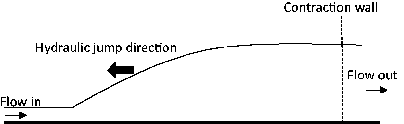

Figure 12 shows the velocity vectors of the central axial plane and the cross sectional velocity vectors before the oblique jump at x = 3.08 m. The air velocity vectors, which are above the water velocity vectors, are negligible. The supercritical velocity has reduced at the oblique jump. Flow depth near to the wall has increased before the oblique jump and flow velocity has decreased in those locations. The fluid velocity direction has turned into the y direction near to the contraction wall. Flow depth also increases in this region.

Figure 12.

Velocity vectors: (a) Velocity vectors of the central axial plane at the oblique jump and (b) cross sectional view of the velocity vectors at x = 3.08 m (before the oblique jump in contraction region).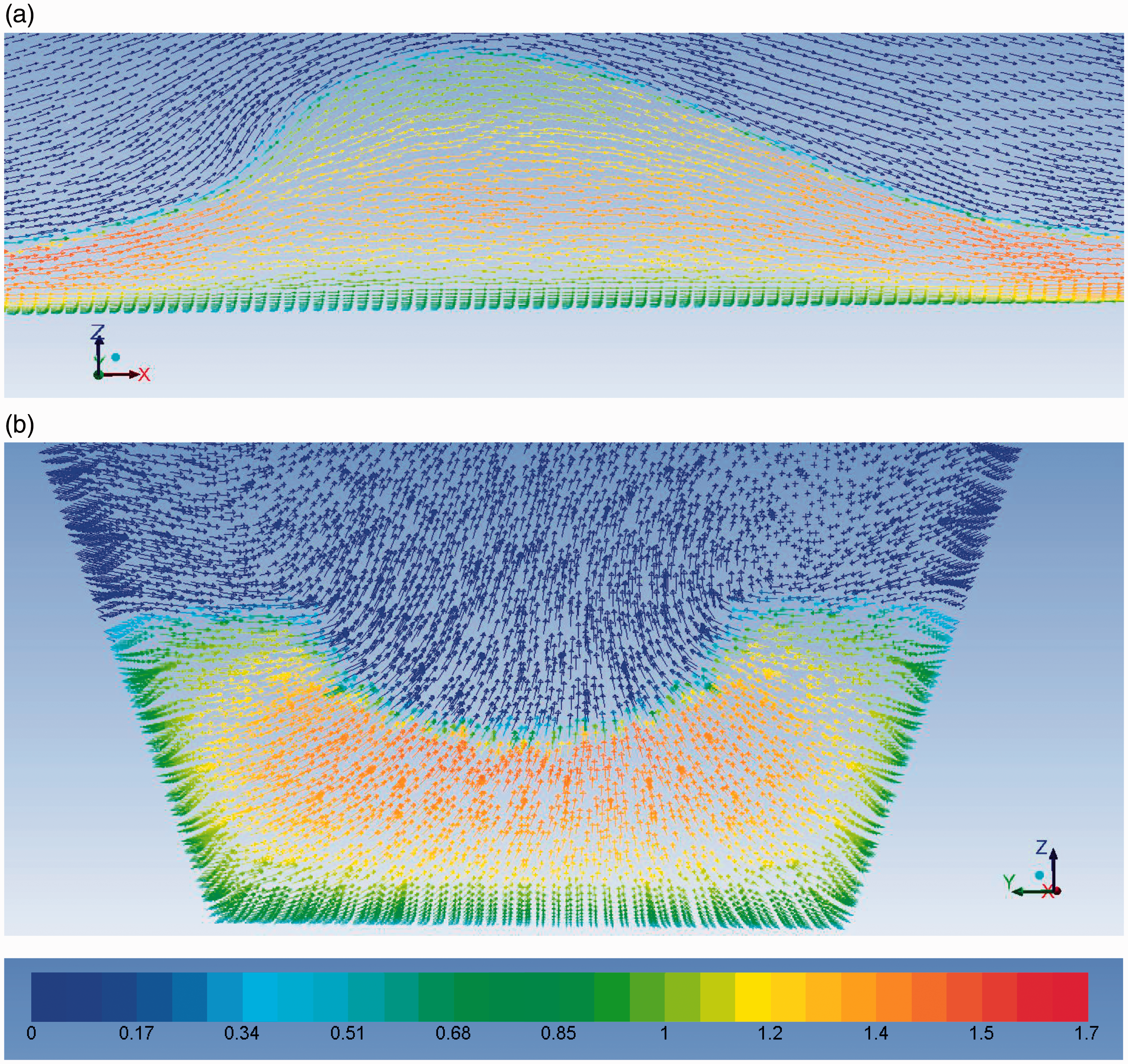

The oblique jump can be demonstrated as shown in Figure 13. There are three jumps meeting in a triple point. j₁ and j₂ jumps are the hydraulic jumps propagated from the contraction walls. In theory, $j_1=j_2$ . The third jump (j₃) is a resultant jump (oblique jump) of these two hydraulic jumps. There are three main flow velocities ( ${\overline{U}}_1,{\overline{U}}_2$ , and ${\overline{U}}_3$ ) and three main flow depths ( ${\overline{h}}_1,{\overline{h}}_2$ , and ${\overline{h}}_3$ ) can be recognized: flow before the hydraulic jump, flow at the hydraulic jump, and flow at the oblique jump. The average flow velocities and average flow depths can be categorized as ${\overline{U}}_1>{\overline{U}}_2>{\overline{U}}_3$ and ${\overline{h}}_1<{\overline{h}}_2<{\overline{h}}_3$ .

Figure 13.

Hydraulic jump arrangement in an oblique jump: Average velocities and average flow depths are shown. 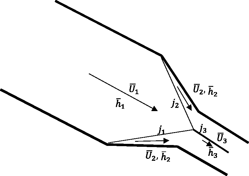${\overline{U}}_1$ and ${\overline{h}}_1$ present before the hydraulic jump. ${\overline{U}}_2$ and ${\overline{h}}_2$ present between wall and hydraulic jump. ${\overline{U}}_3$ and ${\overline{h}}_3$ present at the oblique jump.

Conclusions

An open channel at a horizontal inclination angle gives a subcritical flow until the Venturi contraction wall. After the Venturi contraction, flow transitions into a supercritical flow. For a hydraulic jump to occur in the middle of the channel, the upstream force (friction balancing force coming with upstream fluid) needs to be strong enough to neutralize the hydraulic jump coming to the upstream. The position of the hydraulic jump depends on the balancing of these two forces. As a supercritical flow regime transitions into a subcritical flow regime, a hydraulic jump is generated and flow depth increases. The average velocity in supercritical flow is higher than the average velocity in subcritical flow. When the whole channel flow is at supercritical condition, an oblique jump is generated after the Venturi contraction. The resulting jump of the triple point gives an oblique jump.