A phase-field microscale enhancement for macro models of capillary-driven contact point dynamics

Abstract

We present a method to determine the relation between contact point velocity and contact angle, which can be used as a boundary condition for simulating immiscible and incompressible fluids in contact with solids. The relation is determined from a micro model based on the phase field method. The micro model performs a steady-state computation in a box around the contact point, with far field data given by the macroscale wall contact angle. The size of the micro box is chosen such that physical diffusive processes around the contact point are fully represented. The contact point velocity is shown to converge with respect to the size of the micro box. The angle–velocity relation determined by the micro model is verified on a parameter setting that can be represented by a full phase field simulation.

Introduction

The numerical simulation of incompressible fluid flow with several immiscible fluids is very challenging, both from a methodological and an implementation point of view. A major challenge is the prediction of the physical behavior when the interface that separates two fluids is in contact with a solid and moves, a so-called moving contact line. Applications where the contact line behavior is significant can be found in micro fluidics, coating processes, and biological flows.

The dynamic behavior at contact lines is discussed in recent review articles.^1,2 Typically, the interface forms an angle to the solid that strongly depends on the distance from the contact line. The angle observed on a macroscopic scale, usually referred to as the apparent contact angle, aligns according to the global flow physics. Closer to the contact line one enters the hydrodynamic region where the interface becomes more strongly bent. Here, the interface shape is determined by a balance of viscous and surface tension forces. Even closer to the contact line, within the range of nanometers, molecular fluctuations become important. It is this fine-scale nature of the flow around the contact line that represents a significant numerical difficulty, as it is several orders of magnitude smaller than global flow features in many important applications.

A standard mathematical model for two-phase flow is given by the incompressible Navier–Stokes equations supplemented with jump conditions for the pressure at the interface between the fluids. In a model for moving contact lines, the conventional no-slip boundary condition is not valid, because it would lead to a singularity in the stresses at the contact line. ³ A possibility is to instead use the so-called Navier condition, which relates the slip velocity $\mathbf{u}\text{slip}$ along the wall to the normal strain rate

$$\mathbf{u}\text{slip}=\mathbf{\lambda }\mathbf{n}·(\nabla \mathbf{u}+(\nabla \mathbf{u})\text{T})$$

(1)

Here λ is the so-called slip length, see Davis ⁴ and Spelt. ⁵ The Navier condition works well for flows that are driven by external forces. For capillary-driven flows, the contact angle between the interface and the solid must be explicitly included in the model. This is often done by prescribing the wall contact angle, that is, the microscopic contact angle at the solid wall. Spelt ⁵ proposed to track the contact point explicitly and set its velocity as a function of the contact angle. These and alternative moving contact line models as well as their numerical implementations are discussed in the review article by Sui et al. ⁶

Another possibility is to use the phase field method, where the contact line moves through diffusion. It is based on a phenomenological description using a diffuse interface of finite thickness instead of a mathematically sharp interface. ⁷ The phase field method can handle typical contact line behavior such as advancing or receding motion by virtue of a boundary condition that relates the surface free energy to the contact angle by Young’s relation. ⁷ However, to get reliable results, accurate physical values of the diffusion length and diffuse interface width must be used and the solution must be well resolved. ⁸ Since the diffusion processes around the contact point typically happen on a very small scale whose numerical resolution cannot be afforded for many important settings, it becomes necessary to choose the diffusion length and diffuse interface width as numerical parameters instead. In the context of moving contact lines, adaptive mesh refinement has been demonstrated to represent contact line features that are several orders of magnitude smaller than the simulation domain. ⁶ However, small diffusion length parameters and interface widths at the contact line often translate to high resolution requirements around the interface in the interior of the computational domain for phase field methods as well. More importantly, the representation of fast time scales of contact line diffusion requires the global time step size to be smaller than the diffusion time scale. In the fully adaptive phase field implementation of Ceniceros et al., ⁹ the time step size is proportional to $\Delta x3/2$ , which would lead to prohibitively small time steps in case a physical diffusion length scale were to be resolved.

In this work we determine a relation between contact angle and contact line velocity from a series of microscale simulations of contact line dynamics using the phase field technique. This relation is intended to be used as a boundary condition when simulating immiscible and incompressible fluids in contact with solids on a larger (macro) scale. Our approach uses ideas from matched asymptotics and assumes a temporal and spatial scale separation between the local contact line behavior and global fluid flow. In terms of matched asymptotics, the macroscopic region represents an outer region. The outer solution in the macro model is assumed to exhibit an interface with a well-defined contact angle at the contact line (the apparent contact angle). The inner problem is modeled by the Cahn–Hilliard/Stokes equations, where the effect of a wall is modeled by a standard phase field boundary condition. ¹⁰

We assume the scale separation in space is such that there is a “matching region”, which is close to the contact line at the outer scale and far from the contact line at the inner scale. In the matching region the angle of the interface to the wall varies only very slowly at the inner scale, and we match it to the outer angle (the apparent contact angle). The assumption of the inner interface being essentially planar far from the contact line, supported experimentally, ¹¹ enables us to formulate the inner problem as an initial boundary value problem, with boundary conditions derived from the Huh–Scriven similarity solution. ³ The temporal scale separation means that the time it takes for the inner problem to reach a state of steady movement is small compared to the time scale of the macro flow. This assumption is justified for flows driven by capillary forces. Due to the small length scales in the inner problem, the contact line can be assumed to be essentially straight in the tangential direction to the wall. Thus, the micro model is a two-dimensional problem that considers a single point of contact, referred to as the contact point in the remainder of this work.

The relation we obtain is intended to be used together with some classical scheme on the macroscale, thus providing a procedure for achieving the accuracy of the phase field model with physically relevant parameters in a computationally more efficient framework without excessive grid resolution requirements. The approach inherits the capabilities of the phase field model to treat flows with variable densities, viscosities, or interfacial tension. The simulation domain of the micro model is chosen small enough to represent physical values for the diffusion length scale and diffuse interface width. These parameters have been collected by the phase field community over the last two decades. Our method allows the physical mechanisms described by these parameters to be applied when simulating larger macroscopic flows at a fixed numerical cost.

The proposed method can be interpreted as a variant of a multiscale method. Several multiscale approaches for the contact line problem have been developed in the literature. Hadjiconstantinou ¹² used a molecular dynamics simulation around the contact line, coupled to a continuum description by overlapping domains. In each time step, several iterations were computed on each domain using the results of the other model as boundary conditions until convergence. A more generic approach to couple models based on different physical descriptions at different scales is the heterogeneous multiscale method.^13,14 This method was successfully applied to two-phase flow. ¹⁵ The micro model is usually based on molecular dynamics as in the approach by Qian and co-workers,^16,17 see also their review paper. ¹⁸ For a discussion of different models for contact line dynamics, we refer to Ren and co-workers^19,20 and references therein. All the aforementioned approaches of multiscale models have been applied to two immiscible fluids in Couette or Poisseuille flows with equal fluid densities and viscosities. For more general fluids, multiscale approaches that combine semi-analytical models at the microscale with conventional macroscale solvers have been proposed for droplets moving along walls without contact.^21,22 Macroscale simulations of liquid/gas systems in contact with walls have been enhanced by semi-analytical models at the microscale.^5,6,23,24

The outline of this article is as follows. In the following section, we introduce the phase field model. We formulate a micro problem and describe an algorithm to determine the contact point velocity for a given apparent contact angle. In “Micro results” we present the micro problem results. In “Capillary driven channel flow” we compare the micro results with a simulation of capillary-driven flow using the phase field method. After some time the solution reaches a quasi-steady state, which we compare against the similarity solution. From the transient evolution we have recorded instantaneous contact point velocities and apparent contact angles, which can be compared to the corresponding results from the micro problem. Finally, “Conclusions” summarizes the findings.

Micro model

In this section, we describe the micro model that is used to compute a relation between the apparent contact angle and the contact point velocity. The model is formulated on a small domain near the contact point. The apparent contact angle is the angle between the interface and the solid measured in the macro simulation at a given instant in time. In the setting of this paper, the contact point velocity only depends on the apparent contact angle. It is therefore possible and also most efficient to perform the micro simulation independently of the macro simulation and tabulate the results for use in the macro model.

Phase field method

The phase field model for a system of two immiscible incompressible fluids is based on a mathematical model consisting of the coupled Cahn–Hilliard/Navier–Stokes equations posed on a single domain Ω

$$\frac{\partial c}{\partial t}+\mathbf{u}·\nabla c-m\nabla 2\psi =0$$

(2)

$$\psi -\frac{3\sigma \varepsilon }{4}(\frac{2}{\varepsilon 2}(c3-c)-\nabla 2c)=0$$

(3)

$$\nabla ·\mathbf{u}=0$$

(4)

$$\rho (\frac{\partial \mathbf{u}}{\partial t}+\mathbf{u}·\nabla \mathbf{u})-\nabla ·(2\mu \nabla \text{s}\mathbf{u})+\nabla p=\rho \mathbf{g}+\psi \nabla c$$

(5)

where c is a concentration or order parameter that is +1 and −1 in either fluid with a smooth transition in between. The variable ψ = ψ(c) denotes the chemical potential, and the term c³ − c represents a double-well potential. The Cahn–Hilliard equation (2)–(3) is derived from an interfacial free energy.^10,25 The term $\mathbf{u}·\nabla c$ accounts for convective transport by the fluid velocity u. The variable p denotes the fluid pressure, and $\nabla \text{s}\mathbf{u}=\frac{1}{2}(\nabla \mathbf{u}+(\nabla \mathbf{u})\text{T})$ is the rate of deformation tensor. The parameters $\rho =\rho 1+\frac{1}{2}(\rho 2-\rho 1)(1-c)$ and $\mu =\mu 1+\frac{1}{2}(\mu 2-\mu 1)(1-c)$ represent density and dynamic viscosity, m represents mobility, σ surface tension, and ε controls the diffuse interface width. For a plane interface with normal parallel to the x-direction, the interface profile is given by tanh(x/ε). Our notation can be converted to the notation used in Jacqmin^7,10 with $\psi =\beta (c3-c)-\alpha \nabla 2c$ and parameters $\alpha =3\sigma \varepsilon /4$ and $\beta =3\sigma /2\varepsilon$ . The gravitational acceleration vector is denoted by g and the quantity ψ∇c in the momentum equation (5) represents surface tension. The Cahn–Hilliard equation (2)–(3) is written as a system, which is the form used in the numerical implementation in “Numerical implementation of phase field solver” below.

Boundary conditions supplement the above equations. On a solid boundary (see Figure 1) these conditions are

$$\mathbf{u}=0,$$

(6)

$$\mathbf{n}·\nabla \psi =0,$$

(7)

$$\sigma \varepsilon \mathbf{n}·\nabla c+\cos (\theta \text{S})(1-c2)=0$$

(8)

where n denotes the unit normal vector on the boundary and θ_S denotes the static contact angle between the fluid–fluid interface and the solid, see Jacqmin. ¹⁰ The static contact angle is defined as the angle at which no forces originate from the contact point.

Figure 1.

Sketch of a static interface with the static contact angle θ_S.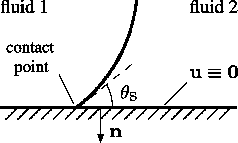

Physics of the micro model

The phase field model allows for contact point motion despite no-slip boundary conditions (6) through diffusive mass transfer around the contact point.^10,26 In the micro model, we use this effect to find a balance between the diffusion and the relative velocity of the interface with respect to the solid, the so-called contact point velocity. The phase field solution is characterized by two inherent length scales.^8,10 The first length scale is the diffuse interface width ε. The mobility m gives rise to the second length scale, the range over which diffusive mass transport is active. In terms of the solution to the Cahn–Hilliard equation, there is a jump in c from +1 to −1 over a range proportional to ε, and the chemical potential ψ is significant in a region of size proportional to m. Hence, interface forces due to contact point dynamics are concentrated to a region whose size is determined by ε and m.

We base the micro simulation on physical values for ε and m for the fluids under consideration. Typical length scales are a few tens to hundreds of nanometers.^10,27 Since we assume the contact region to be small compared to macroscopic length scales, an interface exhibits radii of curvature that are usually much larger than the relevant region for the microscale simulation. In other words, away from the contact point the interface is essentially planar at length scales relevant to diffusive transport. Furthermore, the solution on the micro scale is approximately two-dimensional around the interface. Hence, it suffices to solve the micro problem in two spatial dimensions.

At nanometer length scales, the ratio between viscous and inertial forces in the momentum equation is very high, that is, the Reynolds number is very low, $\text{Re}<<1$ . Thus, we neglect all inertial and gravitational effects in the micro model. In this setting, the Navier–Stokes equations reduce to the Stokes equations with the momentum equation given by

$$-\nabla ·(2\mu \nabla \text{s}\mathbf{u})+\nabla p=\psi \nabla c$$

(9)

and continuity equation according to (4). In our micro model, the Stokes system is coupled to the Cahn–Hilliard equation (2)–(3), and it is time-dependent due to this coupling.

As a computational domain, we choose a rectangular box of height L, which needs to be large enough in order to fully represent the diffusion region in the phase field model. The length of the box is αL, where α is selected large enough to cover the complete interface (including some additional space in order to allow the contact position to develop), and varies with the wall angle θ_a. Figure 2 depicts the computational domain together with the boundary conditions defined in “Boundary conditions for the micro model” below. The flow in the micro model is characterized by the following non-dimensional numbers

$$\mu *=\frac{\mu 1}{\mu 2}\mathrm{\hspace{1em}\hspace{1em}\hspace{1em}}\mathrm{\hspace{1em}\hspace{1em}\hspace{1em}}\hspace{1em}(\text{viscosityratio})\text{Ca}=\frac{U\text{ref}\mu 1}{\sigma }\mathrm{\hspace{1em}\hspace{1em}\hspace{1em}}(\text{capillarynumber})S=\frac{\sqrt{m\mu 1}}{\ell \text{ref}}\mathrm{\hspace{1em}\hspace{1em}\hspace{1em}}(\text{strengthofdiffusivemasstransport})\text{Cn}=\frac{\varepsilon }{\ell \text{ref}}\mathrm{\hspace{1em}\hspace{1em}\hspace{1em}}\hspace{1em}\mathrm{\hspace{1em}\hspace{1em}\hspace{1em}}(\text{Cahnnumber})$$

where μ₁,μ₂ are the dynamic viscosities of fluids 1 and 2, respectively. The velocity scale is chosen as $U\text{ref}=\frac{\sigma }{\mu 1}$ , which normalizes the velocity with respect to surface tension and gives Ca = 1. The diffusion length scale ℓ_ref is chosen as $\ell \text{ref}=\sqrt{m\mu 1}$ , which normalizes the strength of diffusive mass transport at S = 1. Together with the static contact angle, these physical parameters fully describe the Cahn–Hilliard/Stokes system. In our approach, the only numerical parameter is the box height L. We will show convergence of the micro results with respect to L →∞ in “Convergence behavior of micro model.” This means that our micro results do not depend on other numerical parameters, assuming that the phase field parameters ε and m are matched to experimental data in the usual phase field framework.

Figure 2.

Schematic illustration of micro model with boundary conditions. The similarity velocity 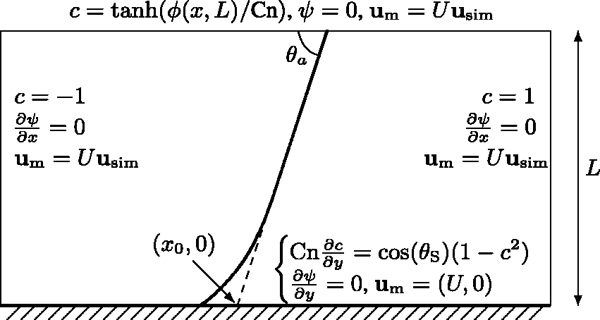u_sim is centered at the point (x₀,0), the extension of a plane interface to the boundary.

Asymptotics of micro model

Our approach is based on ideas from matched asymptotics. ¹ The matching is done at an intermediate mesoscale, which is much smaller than the global length scales of the flow (e.g. scale of droplets), but still much larger than the microscale based on the interface width and diffusion length. On this mesoscale, the macro solution is close to wedge shaped with a well defined contact angle. The flow around a plane interface at zero Reynolds number can be described by the flow model introduced by Huh and Scriven. ³ The Huh–Scriven model gives a similarity solution for the velocity $\mathbf{u}\text{sim}$ based on the apparent contact angle θ_a and the viscosity ratio μ*. The model breaks down close to the contact point because of the singularity in the shear stress. In our micro model the inherent diffusion of the phase field method avoids the stress singularity at the contact point, see also Figure 13 later. There is experimental evidence that the flow at intermediate distance from a contact point is close to the Huh–Scriven similarity solution in Dussan. ¹¹ We therefore match the macro- and microscale solutions by applying the Huh–Scriven similarity solution as a boundary condition at the open boundaries for the microscale problem. Asymptotically we expect the interface of the microscale solution to become increasingly planar far from the contact point. Note that the logarithmic dependence predicted in the literature, see for example Bonn et al. ¹ and Snoeijer and Andreotti, ² which corresponds to viscous bending, is most prominent near the contact point. This effect will, to a large extent, be captured by the micro model.

Boundary conditions for the micro model

Since the velocity field does not decay away from the contact point, we need to define the behavior of the velocity on the boundary of the micro model. We assume that the Huh and Scriven ³ similarity solution is valid in the far field and use it to formulate boundary conditions on the open boundaries of the micro domain. The similarity velocity $\mathbf{u}\text{sim}$ is expanded around the point (x,y) = (x₀,0), the extension of a plane interface to the wall, see Figure 2. Note that the similarity velocity is not related to the interface description by the phase field method, and does not specify values for the variables c and ψ.

As explained above, the purpose of the micro model is to find a contact point velocity U given an apparent wall contact angle θ_a, by considering the flow field in a small domain around the contact point. The contact point velocity U describes the relative motion of the contact point which is in balance with the diffusion in the phase field method when an outer apparent contact angle is prescribed. In order to restrict the simulation to a fixed domain, we let the simulation domain follow the contact point speed U by changing the frame of reference.

The following boundary conditions are set in the micro simulation (compare with Figure 2).

Along the solid wall, we assume the usual phase field boundary condition (7)–(8) together with a convectional no-slip boundary condition (6) for the velocity. Due to the change of frame of reference, the boundary condition is $\mathbf{u}\text{m}|\text{wall}=(U,0)$ .

The velocity field on the open boundaries is set according to the Huh–Scriven similarity velocity, ³ scaled by the velocity of the contact point, $\mathbf{u}\text{m}|\text{open}=U\mathbf{u}\text{sim}$ .

The concentration variable along the upper boundary follows the profile that is attained by plane interfaces, $c(\mathbf{x})=\tanh (\phi (\mathbf{x})/\text{Cn})$ , where φ(x) denotes the signed distance of x from the initial interface. This ensures the interface remains fixed along the upper boundary. At the left and right boundaries, c is set to −1 and +1, respectively. The chemical potential is set to a homogeneous Dirichlet condition at the upper boundary and no-flux (7) at the left and right boundaries, respectively. These conditions ensure the contribution from surface tension to be zero at the open boundaries, as expected for a straight interface.

Since Dirichlet conditions for the velocity are imposed on the whole boundary of the domain, the pressure is only determined up to a constant. We fix the pressure in the lower left corner of the domain to zero.

The simulation is started with a plane interface according to the wall contact angle, see Figure 2, that is, $c(\mathbf{x})=\tanh (\phi (\mathbf{x})/\text{Cn})$ . Note that the wall contact angle θ_a is not directly enforced as a boundary condition in the micro simulation. Nonetheless, we expect the steady-state solution to approach the similarity solution corresponding to θ_a away from the contact point. Correspondingly, the interface will cut the upper boundary with angle θ_a. This behavior has been verified numerically for the final value of U, where approximately the upper half of the interface in the box is essentially straight and aligns at θ_a to within 0.5%.

Numerical implementation of phase field solver

For convenience of implementation, we solve the micro model for a velocity variable u that satisfies zero Dirichlet conditions along the whole boundary also in the moving frame of reference

$$\mathbf{u}=\mathbf{u}\text{m}-U\mathbf{u}\text{sim}$$

(10)

where $U\mathbf{u}\text{sim}$ is the similarity velocity. This introduces additional forcing due to viscous dissipation of the similarity velocity.

We discretize the system (2)–(4) and (9) with the finite element method. To this end, we first write the system in weak form with inner product (·,·)_Ω defined as integration over Ω. The objective is to find functions u,p,c,ψ in suitable Sobolev spaces (weak first derivatives, boundary conditions according to “Boundary conditions for the micro model”) such that

$$(vc,\frac{\partial c}{\partial t}+(\mathbf{u}+U\mathbf{u}\text{sim})·\nabla c)\Omega +(\nabla vc,S2\nabla \psi )\Omega =0(v\psi ,\psi -\frac{3(c3-c)}{2\text{Cn}})\Omega -\frac{3}{4}(\text{Cn}(\nabla v\psi ,\nabla c)\Omega \mathrm{\hspace{1em}\hspace{1em}\hspace{1em}}+(v\psi ,\cos (\theta \text{S})(1-c2))\Gamma \text{wall})=0(vp,\nabla ·\mathbf{u})\Omega =0(\nabla \text{s}\mathbf{v}u,2\nu \nabla \text{s}\mathbf{u})\Omega +U(\nabla \text{s}\mathbf{v}u,2\nu \nabla \text{s}\mathbf{u}\text{sim})\Omega \mathrm{\hspace{1em}\hspace{1em}\hspace{1em}}-(\nabla ·\mathbf{v}u,p)\Omega -(\mathbf{v}u,\psi \nabla c)\Omega =0$$

(11)

holds for all admissible test functions v_c,v_ψ,v_p,v _u . We define a smoothly varying non-dimensional viscosity as $\nu =(1-c)+\frac{\mu *}{2}(1+c)$ , where μ* denotes the viscosity ratio, see “Physics of the micro model.” The domain is subdivided into rectangular elements and the infinite-dimensional spaces are approximated by piecewise polynomial approximations on the elements. For the Cahn–Hilliard variables c and ψ, bi-linear basis functions $\mathcal{Q}1$ on the elements are chosen. For the Stokes system, bi-quadratic ${\mathcal{Q}}_2^d$ elements for velocity and $\mathcal{Q}1$ elements for pressure are chosen, which satisfy the so-called inf–sup condition, see, for example, Gresbo and Sani, ²⁸ and thus give a stable discretization. Equation (11) is then enforced on the finite-dimensional subspaces.

The time derivative is approximated using a backward differentiation formula of order 2 (BDF-2), ²⁹ that is, $\partial cn+1/\partial t\approx (3c(n+1)-4c(n)+c(n-1))/(2\Delta t)$ and the spatial terms are evaluated at time level n + 1. The coupling between the momentum equation and the Cahn–Hilliard equation is resolved by an explicit segregation approach. In one time step, we first solve for the Cahn–Hilliard equation with a velocity extrapolated to the new time level, $\mathbf{u}*=2\mathbf{u}(n)-\mathbf{u}(n-1)$ , and then the Stokes equation with new values for c^{( n +1)} and ψ^{( n +1)}. This avoids solving the coupled Cahn–Hilliard/Stokes system, but introduces a limit on the time step $\Delta t~\frac{\mu }{\sigma }\Delta x$ , see Galusinski and Vigneaux. ³⁰ The nonlinearity in the Cahn–Hilliard equation is resolved with a Newton iteration that typically takes 1–3 steps to converge. The resulting linear system for the Cahn–Hilliard equation is solved with the generalized minimum residual solver and a block preconditioner according to Axelsson et al., ³¹ and the linear system for the Stokes system with a generalized minimum residual solver and a block Schur complement preconditioner according to Silvester and Wathen. ³² The micro solver is implemented in a high-performance C++ code ³³ based on the finite element library deal.II ³⁴ with efficient matrix-free solvers. ³⁵

Micro results

In order to exemplify the numerical algorithm, we provide computational results for water and oil in the next subsections, using the material parameters given in Table 1. The table also indicates the mesh resolution and time step size used in the experiments throughout this section. We use non-dimensional quantities in the simulation. Note that the Cahn number Cn = 1.90 is within the range Cn ≤ 4S identified in Yue et al. ⁸ for convergence at contact points. Since the micro simulation is performed in dimensionless units, its result must be transformed into dimensional values before usage in the macro model. A dimensional contact point velocity is obtained through the relation $U\text{dim}=U\frac{\sigma }{\mu 1}$ , where U is the non-dimensional velocity determined by the micro model.

Table 1.

Parameters for the oil–water case. Note that only the given non-dimensional numbers are used in the computations. The static contact angle is measured from the oil side, that is, water is wetting.

ρ 1	ρ 2	μ 1	μ 2	σ	μ *	Cn	θ S	L	Δx	Δt
$[\frac{\text{kg}}{\text{m}3}]$	$[\frac{\text{kg}}{\text{m}3}]$	$[\frac{\text{kg}}{\text{ms}}]$	$[\frac{\text{kg}}{\text{ms}}]$	$[\frac{\text{kg}}{\text{s}2}]$	–	–	[degrees]	—	–	–
1000	730	0.001	0.00334	0.054	0.299	1.90	140	30	0.5	0.5

Functional relation for contact point velocity

The algorithm outlined in “Numerical implementation of phase field solver” simulates the time-dependent dynamics of two-phase flow for given material parameters and boundary conditions. In our case, we have to find a contact point velocity U for which the phase field simulation reaches a steady state in the moving frame of reference, given an input angle θ_a. This is a problem of inverse type in the control variable U (see Chapter 1 of Hinze et al. ³⁶ ). To identify steady state in a simulation framework, we define a functional expression f = f(U) that evaluates to zero for a contact point velocity U that gives steady state. When the velocity U is too high or too low, a positive and negative value of f is desired, respectively.

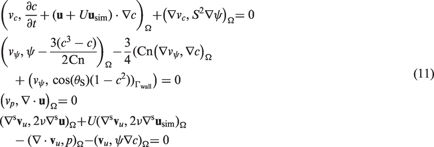
To this end, the function f is defined as the motion of the contact point relative to the moving frame of reference as depicted in Figure 3. As sketched, the contact point moves to the right when the wall velocity U is too low, and to the left if the wall velocity is too high. Figure 4 shows simulation results for the interface shape in the steady-state case, which is the output of the secant method described below. Note that the interface is not planar at the top boundary, but the curvature of the interface increases towards the lower boundary in Figure 4.

Figure 3.

Schematic illustration of reaction to different wall velocities. If the wall velocity U is too low or too high, the interface moves to either right or left. We denote the velocity for which steady state is reached by U_s. Figure 4 shows computational results for this situation. The static contact angle θ_S is assumed to be 140 degrees and the wall contact angle θ_a equals 80 degrees in this illustration.

Figure 4.

Velocity field for phase field simulation using a static contact angle of 140 degrees and a wall contact angle of 80 degrees for the steady state velocity U with f(U) = 0. The interface is indicated by a thick solid line, and the two thin lines give the location of the −0.9 and+0.9 contour lines in the concentration c. The color displays the magnitude of the total velocity field $\mathbf{u}\text{m}=\mathbf{u}+U\mathbf{u}\text{sim}$ .

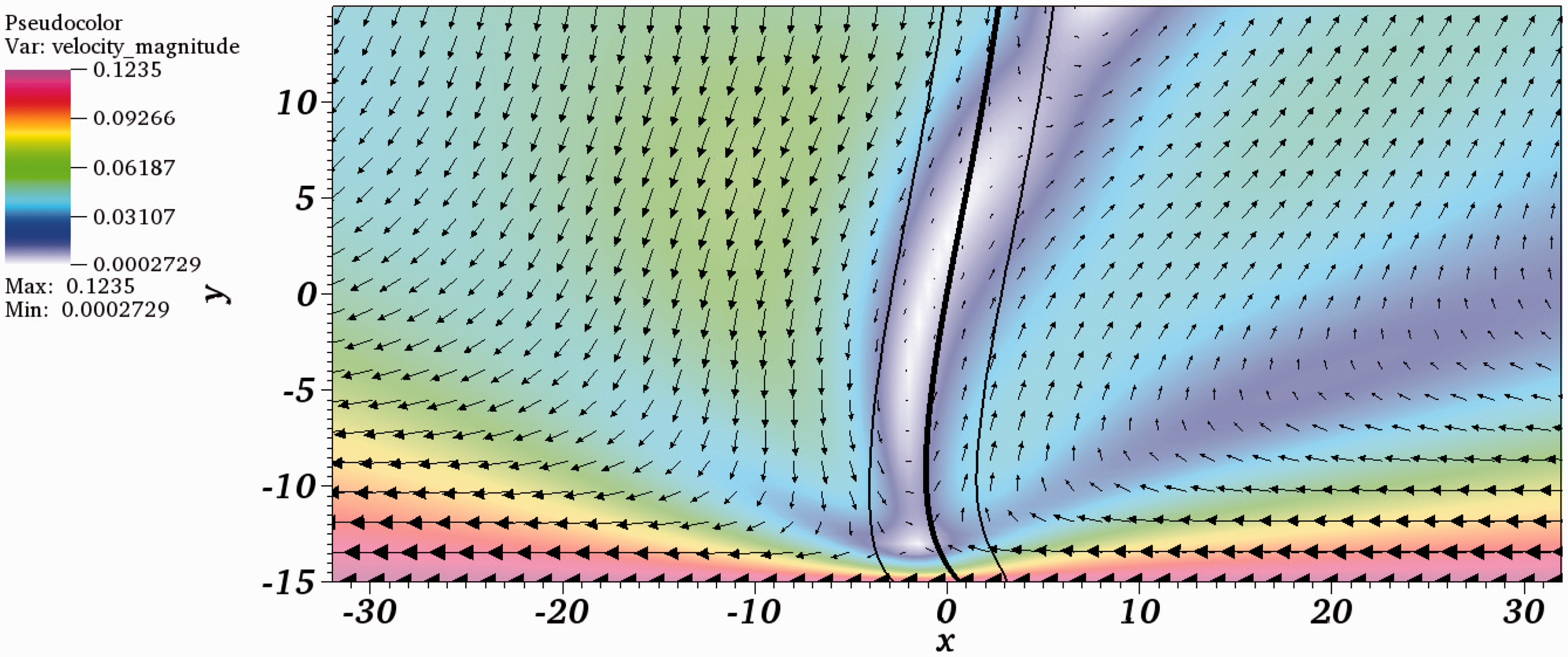
Figure 5 illustrates the behavior of the phase field solution over time for a wall contact angle of 80 degrees and the water–oil material combination. The solid red line shows the time evolution for the numerically computed contact point velocity that yields a steady state, together with two contact point velocities that are too small (contact point drifts to the right) and two cases where the contact point velocities are too large (contact point drifts to the left). Figure 5 also includes the values of function f as the measured contact point velocity against the moving frame of reference for the same situation. The function is monotone in the contact point velocity and there is a distinct zero value, guaranteeing robustness of a root-finding algorithm. We emphasize that the steady state found by our algorithm does not depend on the particular choice of the function f(U). Other one-dimensional quantities that take up the motion of the interface based on the concentration variable c are also possible.

Figure 5.

Development of the interface position at the wall boundary in terms of the given slip velocity U. The materials considered are water and oil with static contact angle equal to 140 degrees (measured from the oil side), and the wall contact angle is equal to 80 degrees. The velocity U = −0.1235 is the solution from the secant method (13). (a) Time evolution of interface position. (b) Functional relation f(U).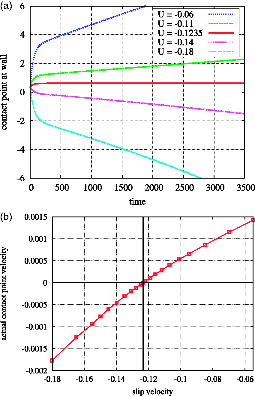

Since system (11) is time-dependent, we need to identify a suitable time for when to record f(U). As can be seen from Figure 5(a), an initial transient is present in the system where the interface changes from the wall contact angle towards the prescribed static contact angle. From non-dimensional time t≈300 onwards, an approximately linear behavior of the contact point position develops. Therefore, it is reasonable to measure the contact point speed during this phase. We choose the final time for the micro simulation to be 10 times the time interval of initial transients, that is, time 3000, when evaluating f(U).

Secant method

For finding the contact point velocity U given a wall contact angle θ_a, the root to the following one-dimensional nonlinear equation must be found

$$f(U)=0$$

(12)

To this end, the secant method is applied. We choose an initial velocity U₀ (result from a simulation with slightly different material parameters, result from a simulation at a neighboring wall contact angle, or simply zero), and a perturbed velocity, for example, U₁ = U₀ + 0.001. The iteration to find the next velocity is then

$$Uk+1=Uk-f(Uk)\frac{Uk-Uk-1}{f(Uk)-f(Uk-1)},\mathrm{\hspace{1em}\hspace{1em}\hspace{1em}}k=1,2,\dots$$

(13)

We stop the iteration as soon as the update U_k+1 − U_k is smaller than a given tolerance of 10⁻⁵. Since we solve the Stokes linear system only approximately with an iterative method, the function value f(U) contains a certain degree of noise, which affects the secant method for small tolerances. We found that solving the Stokes systems to an absolute residual about two orders of magnitude smaller than the secant method tolerance eliminates this influence. In all the experiments reported below, the secant method converged in three to seven steps, which means that not more than eight function evaluations f(U_k) were necessary to find the correct contact point velocity. These good convergence properties are due to the distinct zero in f(U), see Figure 5(b).

Tabulation of micro results

In order to use the micro model for simulations, its information needs to be integrated into a macro simulator. As discussed in the introduction, the approach to measure the angle in the macro model in each time step and then finding U on the fly is very expensive. It involves solving several time-dependent phase field problems in order to find the correct contact point velocity, even when starting with good initial guesses. Therefore, we pre-compute the contact point velocity for a range of wall contact angles and collect the results in a table as $U({\theta }_{\text{a}}^k),k=1,\dots ,N$ . From the table, one can compute U(θ) for an arbitrary θ by interpolation. The resulting graph for water and oil is shown in Figure 6.

Figure 6.

Contact point velocities for oil/water material combination for different sizes of the simulation domain L. The mesh size is set to h = 0.5 and the time step Δt = 0.5. (a) Full range of contact angles. (b) Zoom around static contact angle.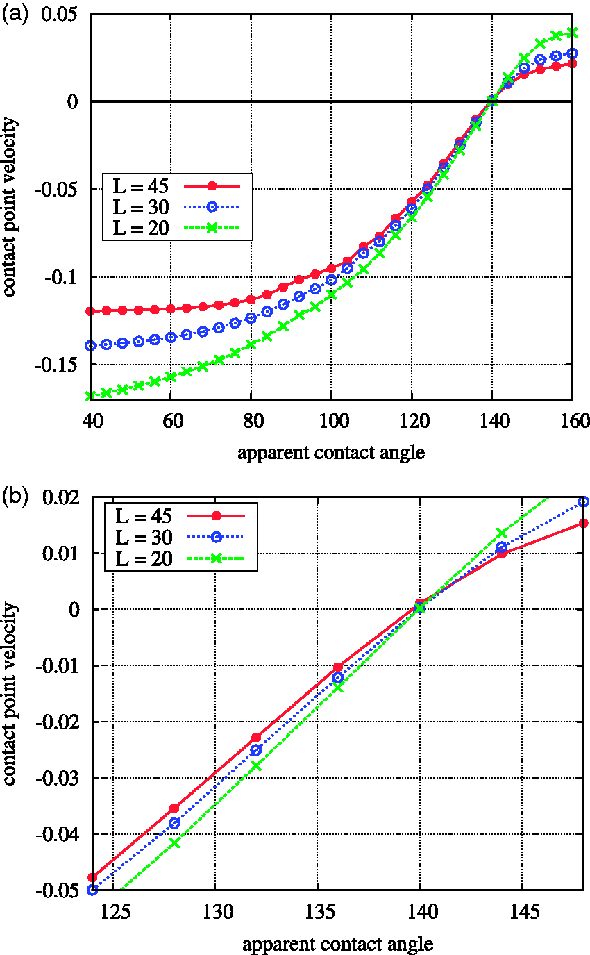

Convergence behavior of micro model

In order to obtain accurate results for the contact point velocity U in the micro solver, we need to ensure that the discretization resolves the physical features of the flow and that the diffusion along the contact point is captured by the diffuse Cahn–Hilliard interface, as explained in Yue et al. ⁸ We performed extensive convergence studies to verify that the chosen values of Δx and Δt adequately resolve the interface dynamics of the phase field parameters given in Table 1 with deviations in the resulting contact point velocity of 0.2% or less. In a second set of computations, we analyze the dependence of the contact point velocity on the height of the micro box L while keeping S, Cn, Ca fixed. Figure 6 shows the resulting contact point velocity U for three particular values of the height, L = 20, L = 30, and L = 45. The solutions for L = 30 and L = 45 are in close agreement, especially in the region between 120 and 140 degrees.

Figure 7 shows the contact point velocity for the apparent contact angle of 80 degrees over a larger range of the box height. The plot demonstrates that the computed contact point velocity converges to a value that is independent of box size as the box size increases, which supports omitting the weak logarithmic dependence of the angle in the matching procedure. In terms of the results presented in Figure 13 later, an increasing box size gives a larger region which matches with the similarity solution. We observe a similar convergence behavior for other apparent contact angles and material parameters. We have also seen that convergence in the far field to the similarity solution seemed to be enhanced by increasing the box size.

Figure 7.

Contact point velocity U for different sizes of the micro box L for apparent contact angle equal to 80 degrees. The mesh size is set to h = 0.5 and the time step size Δt = 0.5.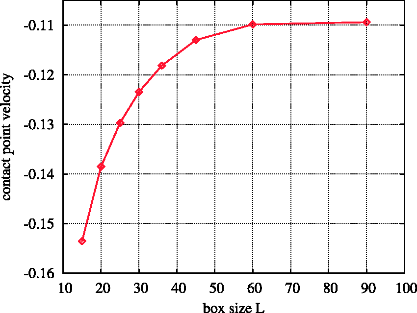

Figure 8 compares the contact point velocity for our method using L = 30 with Cox’ relation ³⁷ for oil and water. A scaling parameter $\varepsilon =\frac{1}{4}$ was used in the expression ln(ɛ⁻¹) of Cox’ relation (7.22) ³⁷ to obtain the same slope around the static angle of 140 degrees as our method. The result shows that our method produces a considerably smaller slope than Cox’ relation for large deviations from the static contact angle. This can be explained by the relatively large value of ɛ in Cox’ relation necessary to fit the slope of our results around θ = 140 degrees. On the other hand, we expect our method to include more physical mechanisms than the Cox model which is based on lubrication theory.

Figure 8.

Contact point velocity U for our method at L = 30 and the prediction by Cox’ law.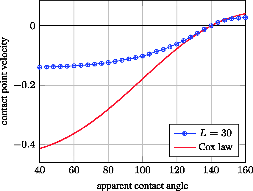

Capillary driven channel flow

In this section we relate the results of the micro simulation to a full phase field simulation of capillary dominated channel flow. We consider capillary rise in a horizontal channel. For the test, non-dimensional quantities are set in the solver as m = 1, ρ₁ = 1, ρ₂ = 0.73, μ₁ = 0.3, μ₂ = 1, σ = 1 with the static contact angle θ_s = 140°, measured from fluid 2 (compare with physical data in Table 1). We will consider channel height d = 20,40. In both cases the regions near the wall where the mass diffusion is important are of size ∼1, and are smaller than the full channel width. The channel length is denoted by L. The pressure is fixed to zero at the inlet and outlet and no gravity acts on the fluids. Initially the interface between the two fluids is a straight line at x = 25 with fluid 1 placed to the left of the interface. After an initial transient, the system develops into a quasi-steady state where the interface moves with a fixed velocity. The steady-state flow is determined by a balance of the capillary forces against the viscous stress in the fluids. The longer the channel, the slower the contact point velocity. Figure 9 displays the measured contact point velocity as a function of time for the length L = 120 for the d = 20 case. Note that the acceleration of the contact line in the later stage of the simulation is because the more viscous fluid 2 is displaced by the less viscous fluid 1. The mesh size is chosen as $h=\frac{20}{512}\approx 0.04$ (giving around a million elements), the Cahn number is Cn = 0.11 and the time step size Δt = 0.1.

Figure 9.

Contact point velocity U as a function of time for the channel length L = 120.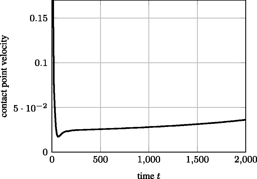

Angle-velocity relation

We have also measured the apparent angle and contact point velocity in the full phase field solver for comparison with our computed relation from the micro solver. The velocity of the interface is easily computed as the motion of the contact point along the wall according to Figure 9. The apparent angle is more difficult to assess. The interface is bent close to the contact point due to the diffusive mass transport. Therefore, the measurement of the contact angle must be based on the shape of the interface at some distance away from the contact point.

We can compute the curvature at different positions along the interface by considering the position of the zero contour in the phase field variable c as a function of the vertical coordinate y. Since the simulation output of the interface are line segments, a higher order interpolation needs to be done first. We achieve this by computing a cubic spline interpolation s(y) of the interface data, which gives the interface curvature by

$$\kappa (y)=\frac{s″(y)}{(1+(s\text{'}(y))2)3/2}$$

(14)

Figure 10 displays the interface curvature (14) for five simulation settings in the d = 20 case. Note that in Figure 10 the interface is essentially circular in the central part of the domain, at least for the larger lengths of the channel, which correspond to small or moderate velocities of the contact point. This is not surprising as a circle is a steady-state solution. Based on an averaged curvature $\overline{\kappa }$ , measured at a distance y⁺= y + 10 between 8 and 12, a circle is constructed. In the d = 20 case this corresponds to the central part of the domain, and the interface angle is computed from this circle extrapolated to the domain boundary

$$\theta \text{a}=\arcsin (10\overline{\kappa })$$

where 10 is the half channel height. In the d = 40 case we base the angle on a circle constructed from the shape of the interface at the same distance y⁺ from the wall.

Figure 10.

Curvature according to equation (14) as a function of the vertical position y.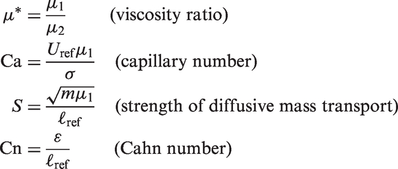

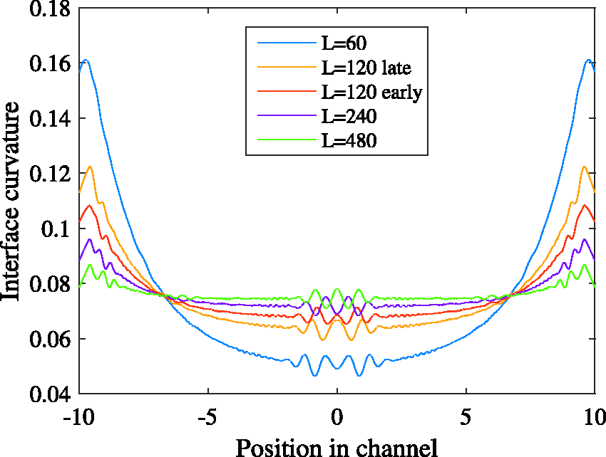
Figure 11 compares measurements of the velocity and interface angle in the full phase field simulation with the results from the micro simulation in Figure 8. The five red points are based on d = 20 and the four different channel lengths L as depicted in Figure 10 are L = 60, L = 120, L = 240, and L = 480. For the case L = 120, the angle–velocity relation is recorded at two different instants in time, one at t = 100 and one at t = 1200 where the interface is located around x = 29.0 and x = 58.4, respectively. At the later time, the amount of the more viscous fluid has decreased, increasing the contact point velocity and reducing the apparent contact angle as visible from Figure 10. The comparison shows that the measured velocities at the contact point are in close agreement with the prediction of the micro model.

Figure 11.

Comparison between micro model and actual phase field results.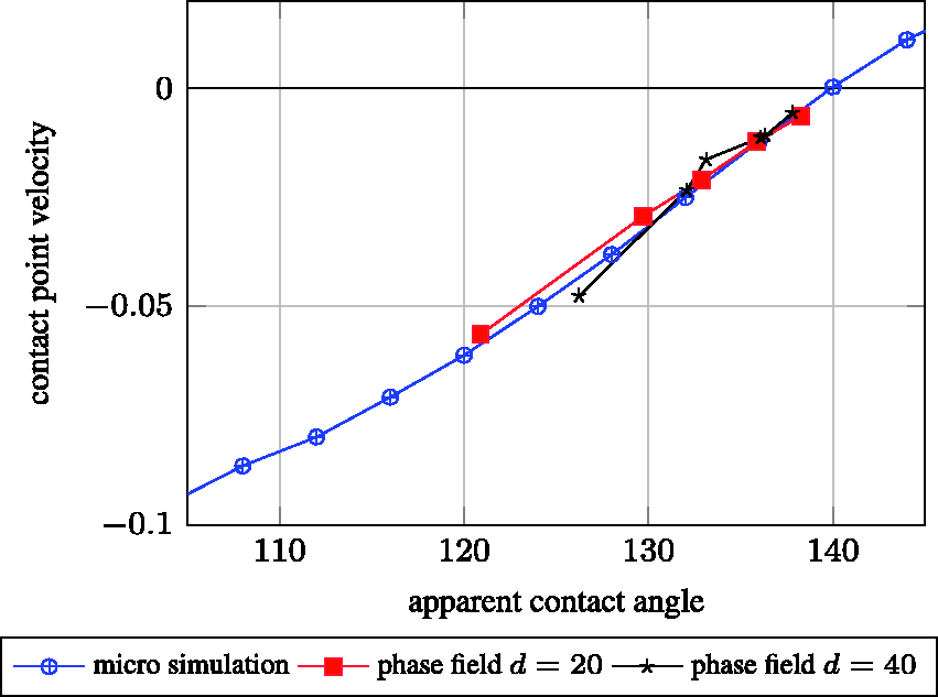

Figure 11 also includes results of a second phase field simulation employing a larger channel height d = 40, given by the black points. As mentioned above, the angle measurements are based on a fit of a circle at wall distance between 8 and 12. As before, four channel lengths L = 120, 240, 480, 960 as well as two different times for checking the velocity at L = 240 and L = 480 have been selected, giving six data points. The results again show very good agreement with the micro simulation.

Quasi-steady state

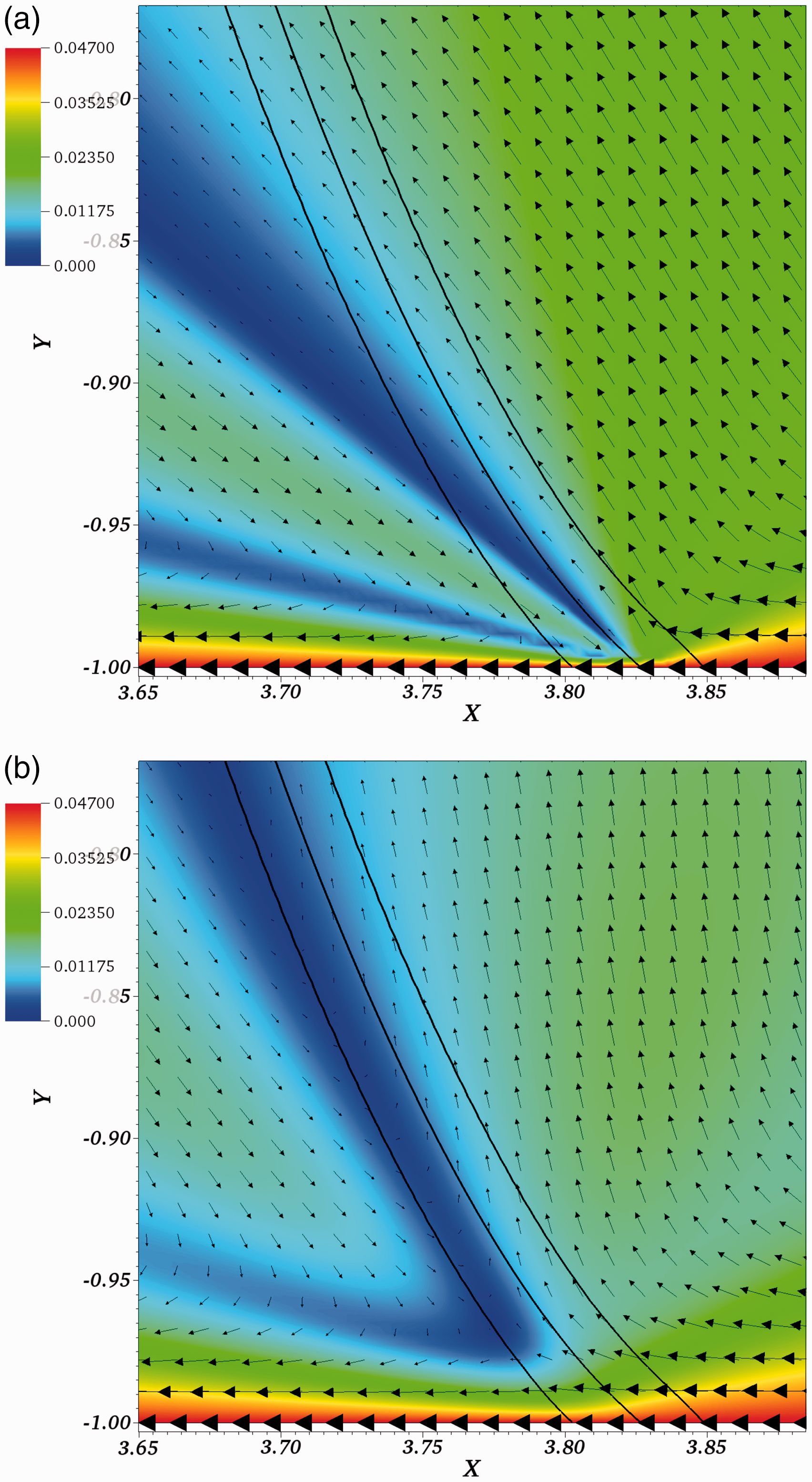
After the initial transient the phase field solution approaches a quasi-steady state, see Figure 12. We compare the velocity field from the phase field simulation with a corresponding similarity solution in Figure 13. The phase field simulation shows a good qualitative agreement of velocity directions. There are two main deviations between the two fields. Firstly, the diffuse transport around the interface for the phase field model removes the singularity in the similarity velocity and contributes to a smooth transition of no slip at the wall (corresponding to velocity fields pointing to the left in the moving frame of reference) and the static interface position. Secondly, the true interface is not flat, and therefore deviates from the flat similarity solution interface.

Figure 12.

Velocity field and interface position as the contact point passes x = 50.

Figure 13.

Velocity fields in moving frame of reference, comparing the Huh–Scriven similarity velocity field ³ attached to the numerically computed contact point position and apparent contact angle of 137.41 degrees with the actual velocity field in a phase field simulation. The three black lines show the location of the ±0.9 and 0 contour lines of the phase field variable c. (a) Similarity velocity field. ³ (b) Phase field simulation of velocity field.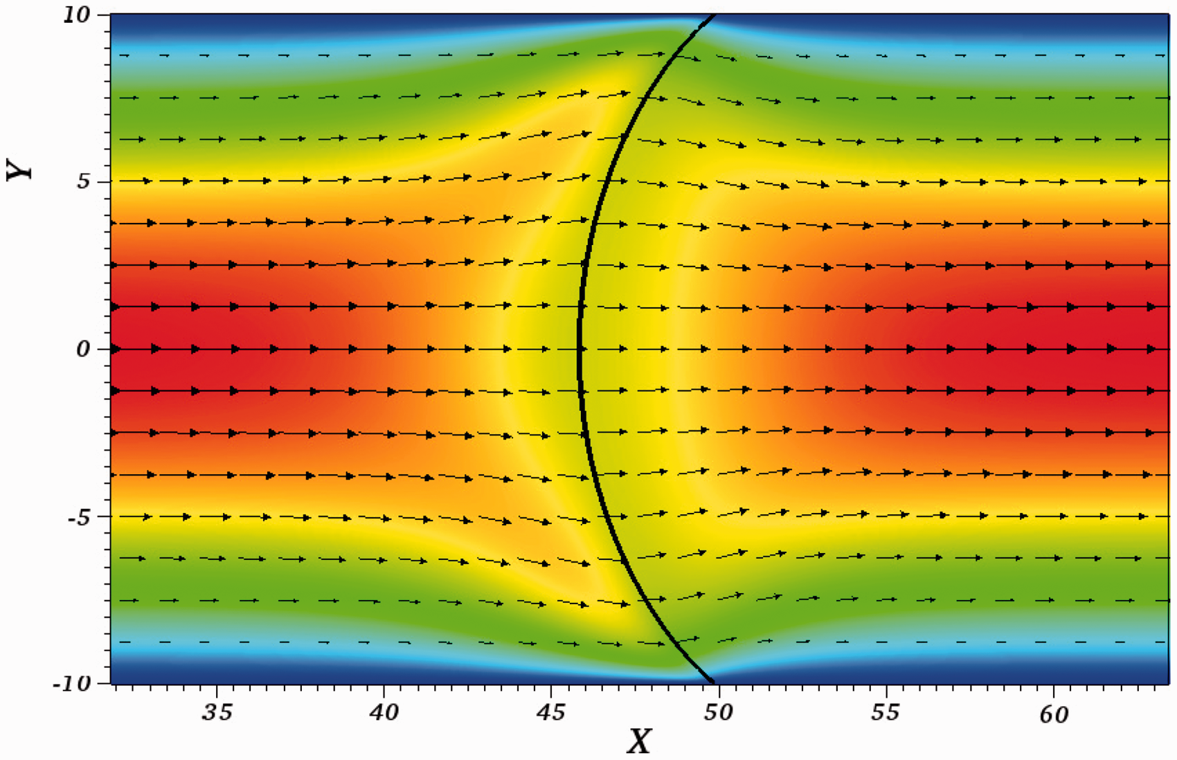

Conclusions

We have presented an algorithm for computing a relation between the contact point velocity and the wall contact angle, to be used as a boundary condition for simulation of the flow of two immiscible incompressible fluids with moving contact lines, on scales significantly larger than micrometers.

The relation between the contact point velocity and the wall contact angle was determined by considering a so-called micro model, which is based on the response of the flow to the molecular forces induced by the macroscopic contact angle. The dimensions of our micro simulation can be adjusted to physical length scales over which contact point diffusion occurs by choosing appropriate non-dimensional material parameters in the micro model. The micro model was used to tabulate the relation between the contact point velocity and the wall contact angle for a given material combination. The results of the micro simulation have been validated by comparing with full phase field simulations.

Our approach enables incorporation of the effects of small scale physical diffusion processes around the contact point at real material parameters into conventional macroscale techniques like the level set method, without the high resolution requirements of a straight forward full phase field simulation. Important to note is that considerably coarser meshes can be used for the macroscale simulations than for comparable global phase field simulations, which gives tremendous improvements in computational efficiency.