Sage Journals: Discover world-class research

Abstract

Estimating distance traveled is a frequently arising problem in robotic applications designed for use in environments where GPS is only intermittently or not at all available. In UAVs, the presence of weight and computational power constraints makes it necessary to develop odometric strategies based on minimilastic equipment. In this study, a hexarotor was made to perform up-and-down oscillatory movements while flying forward in order to test a self-scaled optic flow based odometer. The resulting self-oscillatory trajectory generated series of contractions and expansions in the optic flow vector field, from which the flight height of the hexarotor could be estimated using an Extended Kalman Filter. For the odometry, the downward translational optic flow was scaled by this current visually estimated flight height before being mathematically integrated to obtain the distance traveled. Here we present three strategies based on sensor fusion requiring no, precise or rough prior knowledge of the optic flow variations generated by the sinusoidal trajectory. The “rough prior knowledge” strategy is based on the shape and timing of the variations in the optic flow. Tests were performed first in a flight arena, where the hexarotor followed a circular trajectory while oscillating up and down over a distance of about $50$ m under illuminances of $117$ lux and $1518$ lux. Preliminary field tests were then performed, in which the hexarotor followed a longitudinal bouncing $20 m$ -long trajectory over an irregular pattern of grass.

Keywords

Optic Flow oscillations visual odometry hexarotor SOFIa indoor and outdoor flight tests aerial field robotics

Introduction

Estimating distance traveled by an aerial robot is a problem which frequently arises when designing applications for use in situations where GPS is available only intermittently or not at all. In UAVs (Unmanned Aerial Vehicles), reducing the Size, Weight and Power (SWaP) of the perceptual equipment is often of great importance in order to ensure that the robot’s task will be performed successfully.

Several visual odometric approaches involving the use of either optic flow,^1,2 events, images & IMU (Inertial Measurement Unit) combinations³ or the sparse-snapshot method⁴ have been successfully tested on flying robots. All these approaches require ground height information providing the factor used to scale the visual information. This scaling factor can be determined separately using a static pressure sensor⁵ or stereovision,^1,4 or it can be integrated when using the hybrid approach,³ for example. One of the approaches used to estimate the 2D position of a drone is a combination of onboard odometry and visual mapping, known as SLAM (Simultaneous Localisation and Mapping).^6–8 Most of these approaches require the use of computationally intensive algorithms and feedback from the environment (such as the detection of a beacon or feedback from a map). A minimalistic alternative is IMU based dead reckoning – i.e. inertial integration.⁹A dead reckoning signal could be used by a UAV to return to the close proximity of its base station before reaching it a second time using other means of perception. In this case, the landing of the UAV on its base station can provide a new known starting point. Another minimalistic alternative consists in using optic flow cues, such as translational optic flow and optic flow divergence cues. Translational optic flow has been used on UAVs to control landing visually,¹⁰ to follow uneven terrain¹¹ and to attempt visual odometry and localisation^12,13 (see Serres and Ruffier¹⁴ for a review).

Self-oscillations have been observed in honeybees flying forward in horizontal,^15,16 doubly tapered¹⁷ and high-roofed^18,19 tunnels. The Self-oscillatory motion generates a series of expansions and contractions in the optic flow vector field, providing the optic flow divergence cue. Visually controlled landing has been achieved based on the optic flow divergence cue.^20–23 The instabilities due to oscillatory movements have been used to determine the flight height of a micro-flyer based on the linear relationship between the oscillation and the fixed control gain.²² The instabilities due to depth variations have been used to assess the optic flow scale factor of the scene observed to perform visual odometry onboard an underwater vehicle.²⁴ The local optic flow divergence was measured by means of two optic flow magnitudes perceived by two basic optic flow sensors placed on a chariot performing back-and-forth oscillatory movements in front of a moving panorama.²⁵ The local optic flow divergence was then used to estimate the local distance between the chariot and the moving panorama by means of an Extended Kalman Filter (EKF).²⁵ A SOFIa (Self-scaled Optic Flow time-based Integration) model has been previously tested as a means of modeling the visual odometer of honeybees with simulations²⁶ as well as with preliminary indoor flights.²⁷ The SOFIa method to estimate the distance traveled is based on the integration of the local translational optic flow scaled by the drone’s flight height, determined by means of an EKF taking the local optic flow divergence as measurement.²⁶ The SOFIa model was found to be about 10 times more accurate than the values obtained in simulations based on the raw mathematical integration of the optic flow.²⁶ Using an integration scheme of this kind can therefore be regarded as a minimalistic dead reckoning method based on the optic flow.

Here we investigated how to include some knowledge about the oscillations occurring during the trajectory in an odometric strategy based on optic flow cues alone. For this purpose, the optic flow based odometric scheme called SOFIa was tested both indoors and outdoors on a hexarotor equipped with optic flow sensors (see Figure 1).

First we applied the SOFIa method using only 2 optic flow measurements perceived along the longitudinal axis of the drone, with no prior knowledge of the optic flow variations. In order to improve the odometric accuracy, a sensor fusion strategy based on the parameters of the self-oscillation using 4 optic flow sensors embedded in the hexarotor was then tested. The idea was to use some prior knowledge about the oscillations imposed on the drone in order to measure the optic flow divergence and the translational optic flow cues more accurately. Two different sensor fusion strategies, based on precise and on rough prior knowledge of the optic flow variations, respectively, were tested. The sensor fusion strategy based on rough prior knowledge consisted solely in using the shape and timing of the variations in the optic flow. All three optic flow based odometric processing methods were tested first indoors on bouncing circular trajectories about $50$ m-long under illuminances of $117$ lux and $1518$ lux and then outdoors on bouncing longitudinal trajectories about $20$ m-long in the presence of various wind and irregular grass conditions.

In section 2., the hexarotor used to perform both indoor and outdoor experiments is described. In section 3., the measurement of the local translational and divergence optic flow cues is discussed. In section 4., the minimalistic visual odometric method is discussed. In section 5., the odometric processing method based on raw measurements of 2 optic flow sensors without any prior knowledge of the optic flow variations is discussed. In section 6., the sensor fusion odometric processing method based on 4 optic flow sensors is discussed, both with precise and with rough prior knowledge of the optic flow variations. In section 7., the indoor experimental setup is first described, and experiments are then presented showing that the two sensor fusion strategies based on the knowledge of optic flow variations increased the measurement quality of the local optic flow cues. Lastly, the performances of the three minimalistic in-flight optic flow based odometric processing methods are compared. In section 8., we first discuss the outdoor experimental setup and then present experiments showing that the same considerations also apply to preliminary flight tests performed outdoors. In section 9., conclusions are drawn and projects for future studies are discussed.

The SOFIa hexarotor

The hexarotor was developed together with Hexadrone $^{TM}$ and equipped with 4 Pixart PAW3903 optic flow sensors (see Figure 2 and Table 1). The Pixart PAW3903 optic flow sensors were embedded on printed circuits to be set on the drone. The hexarotor’s onboard low-level flight controller was the PX4 autopilot system,²⁸ using a trajectory tracking algorithm¹ . Based on the intrinsic attitude stability of the hexarotor, we can assume that no rotational component is measured by the optic flow sensors. In addition, the pitch and roll components were taken to be negligible. The downward translational optic flow can therefore be measured along the $x$ axis of the optic flow sensors.

Figure 2.

(a) Hexarotor equipped with 4 optic flow sensors oriented towards the ground flying along a bouncing circular trajectory in the Mediterranean Flight Arena. (b) 2 optic flow sensors were set along the longitudinal axis $x$ at angles $ϕ = \pm 30^{\circ}$ with respect to the hexarotor’s vertical axis $z$ , while the other 2 optic flow sensors were set along the lateral axis $y$ at angles $ϕ = \pm 30^{\circ}$ with respect to the axis $z$ . (c) Example of a flight test trajectory over a distance of $53$ m at an oscillation frequency of $0.28$ Hz.

Table 1.

Characteristics of the optic flow sensors equipped on the hexarotor.

Specifics	Optic flow sensors
Sensor chip	Pixart PAW3903
Sensor PCB	4 $\times$ 2 g
Hardware read-out of the 4 sensors	Arduino Nano

Measurement of the local optic flow cues

The translational optic flow is the angular speed magnitude of the optic flow vector field generated by the translational motion of a drone flying above the ground.²⁹ The theoretical local translational optic flow $ω_{T}^{t h}$ can be expressed as the ratio between the $V_{x}$ component of the drone’s velocity and its flight height $h$ (see Figure 1):

ω_{T}^{t h} = \frac{V_{x}}{h}

(1)

The local translational optic flow can be measured on a hexarotor as the sum of two optic flow magnitudes

ω (ϕ)

and

ω (- ϕ)

perceived by two optic flow sensors oriented at angles

\pm ϕ

with respect to the hexarotor’s vertical axis, divided by a known factor of

2 \cdot \cos^{2} ϕ

(see mathematical proof in Appendix C):

ω_{T}^{m e a s} = \frac{ω (ϕ) + ω (- ϕ)}{2 \cdot \cos^{2} ϕ} = \frac{V_{x}}{h}

(2)

In the case of a hexarotor equipped with 4 optic flow sensors as illustrated in Figure 2(b), three translational optic flow cues can be measured as follows:

the sum of the two optic flow magnitudes perceived by the two optic flow sensors set along the longitudinal axis $x$ , namely $ω_{T_{1}}^{m e a s}$ ,

the sum of the two optic flow magnitudes perceived on the $x$ axis by the two optic flow sensors set along the lateral axis $y$ , namely $ω_{T_{2}}^{m e a s}$ ,

the median value of the four optic flow magnitudes sensed along the hexarotor’s longitudinal axis by the 4 optic flow sensors, scaled by a $1 / \cos (ϕ)$ factor, namely $ω_{T_{3}}^{m e a s}$ .

The series of contractions and expansions generated in the optic flow vector field by up-and-down oscillatory movements is known as the optic flow divergence. When a drone flies forward while oscillating up and down above the ground, the optic flow divergence is superimposed on the translational optic flow in the optic flow vector field. Due to the oscillatory movements, the state vector

X = [h, V_{h}]^{T}

is locally observable.²³ The theoretical local optic flow divergence

ω_{d i v}^{t h}

can be expressed as the ratio between the

V_{h}

component of the drone’s velocity and

h

(see Figure 1):

ω_{d i v}^{t h} = \frac{V_{h}}{h}

(3)

We have previously proved mathematically that the local optic flow divergence can be measured on a micro-flyer as the difference between two optic flow magnitudes

ω (ϕ)

and

ω (- ϕ)

perceived by two optic flow sensors oriented at angles

\pm ϕ

with respect to the normal to a surface, divided by a known factor of

\sin 2 ϕ

(see mathematical proof in Appendix C)²⁵:

ω_{d i v}^{m e a s} = \frac{ω (ϕ) - ω (- ϕ)}{\sin 2 ϕ} = \frac{V_{h}}{h}

(4)

In the case of a hexarotor equipped with 4 optic flow sensors, two optic flow divergence cues can be measured as follows:

the difference between the two optic flow magnitudes perceived by the two optic flow sensors set along the longitudinal axis $x$ , namely $ω_{{d i v}_{x}}^{m e a s}$ ,

the difference between the two optic flow magnitudes perceived by the two optic flow sensors set along the lateral axis $y$ , namely $ω_{{d i v}_{y}}^{m e a s}$ .

Figure 1.

Hexarotor oscillating up and down while flying forward over the ground at the flight height $h$ . (a) The hexarotor’s velocity $V$ can be decomposed into the components $V_{x}$ and $V_{h}$ . Along the hexarotor’s longitudinal axis $x$ , the optic flow sensors are set at angles $\pm ϕ$ with respect to the hexarotor’s vertical axis, at the distance $D$ with respect to the ground. They perceive the optic flow magnitudes $ω (ϕ)$ and $ω (- ϕ)$ , respectively. This configuration is also present along the hexarotor’s lateral axis $y$ . (b) If $V_{h}$ is positive, the optic flow divergence component is a contraction (in blue) (i); if it is negative, the optic flow divergence component is an expansion (in blue) (ii). The contraction or expansion of the optic flow is superimposed in the ventral optic flow vector field on the translational optic flow (in red).

The SOFIa visual odometer method

A model for the honeybee’s visual odometer called SOFIa (Self-scaled Optic Flow time-based Integration model) was tested in simulations.²⁶ The SOFIa model is based on the integration of the local translational optic flow $ω_{T}$ scaled by the estimated distance with respect to the ground $\hat{h}$ :

{\hat{X}}_{S O F I a} = \int ω_{T} \cdot \hat{h} d t

(5)

\hat{h}

was estimated by means of an EKF. The use of an EKF was necessary due to the non-linearity of the local optic flow divergence, as the measurement depends on the ratio between the two states

V_{h}

and

h

(see equation (3)).

State space representation of the hexarotor along the vertical axis: The hexarotor’s system was modeled in the form of a double integrator receiving as its input the acceleration $a_{z}$ on the vertical axis $z$ given by the drone’s IMU. The hexarotor’s state space representation can therefore be expressed as follows:

{\begin{matrix} \dot{X} = f (X, a_{z}) = A \cdot X + B \cdot a_{z} = [\begin{matrix} 0 & 1 \\ 0 & 0 \end{matrix}] \cdot X + [\begin{matrix} 0 \\ 1 \end{matrix}] \cdot a_{z} \\ \begin{matrix} Y = g (X) = [X (2) / X (1)] = V_{h} / h = ω_{d i v} \end{matrix} \end{matrix}

(6)

where

X = {[\begin{matrix} h, V_{h} \end{matrix}]}^{T}

is the hexarotor’s state vector.

Odometric method based on 2 optic flow sensors with No Prior Knowledge (NPK) of the optic flow variations

The local optic flow divergence $ω_{d i v}^{2 S}$ was measured by taking the difference between the two raw optic flow magnitudes perceived by the 2 optic flow sensors set along the $x$ axis, while the local translational optic flow $ω_{T}^{2 S}$ was measured in the form of their sum. To estimate the flight height $\hat{h}$ , the EKF received the following:

input: the acceleration of the drone $a_{z}$ ,

measurement: the local optic flow divergence $ω_{d i v}^{2 S}$ .

See Appendix B for the EKF calculations.

$\hat{h}$ was then used to scale the integration of the local translational optic flow $ω_{T}^{2 S}$ in order to perform the odometry. This odometric method based on 2 raw optic flow measurements does not require any prior knowledge about any parameters to assess the distance traveled.

Fusion strategies based on 4 optic flow sensors

6.1. Fusion strategy using Precise Prior Knowledge (PPK) of the optic flow variations

Here we investigated how to use prior knowledge about the self-oscillations to further improve the accuracy of the distance traveled estimates with 4 optic flow sensors.

The optic flow divergence induced by the self-oscillation serving as an input to a Kalman Filter (KF) was expressed as follows (see Figure 4(a)):

ω_{d i v} = \frac{\dot{h}}{h} ⟶ U_{d i v} (k) = \frac{A_{o s c} 2 π f_{o s c} \cos (2 π f_{o s c} k δ t)}{h_{0} + A_{o s c} \sin (2 π f_{o s c} k δ t)}

(7)

where

f_{o s c}

, the oscillation frequency, was equal to

0.28

Hz,

A_{o s c}

, the oscillation amplitude, was equal to

0.25

m, and

h_{0}

, the average flight height, was equal to

0.55

m. To fuse

ω_{{d i v}_{x}}^{m e a s}

and

ω_{{d i v}_{y}}^{m e a s}

, a KF was used (see Figure 3). At each

k^{t h}

step, the KF received as input the current value of the model in the equation (7) and as measurements

ω_{{d i v}_{x}}^{m e a s}

and

ω_{{d i v}_{y}}^{m e a s}

. See Appendix A for the KF calculations.

Figure 3.

(a) The sensor fusion based on 2 Optic Flow (OF) sensors is achieved using an Extended Kalman Filter (EKF). The embedded computer handles the outputs of the optic flow sensors set on the hexarotor, whose outputs are used to measure the local optic flow divergence $ω_{d i v}^{2 S}$ and the local translational optic flow $ω_{T}^{2 S}$ . The EKF receives as its input the hexarotor’s acceleration $a_{z}$ and as its measurement $ω_{d i v}^{2 S}$ to estimate the current flight height $\hat{h}$ . The EKF output $\hat{h}$ scales $ω_{T}^{2 S}$ , which is then integrated in order to perform the odometry. (b) The sensor fusion based on 4 optic flow sensors is achieved by inserting additional Kalman Filters (KF). $ω_{{d i v}_{x}}^{m e a s}$ and $ω_{{d i v}_{y}}^{m e a s}$ are taken as measurements by a KF (denoted $K F_{d i v}$ ) receiving as its input the current value $U_{d i v}$ of the model for the optic flow divergence. The output of the KF is the local optic flow divergence $ω_{d i v}^{K F}$ . $ω_{T_{1}}^{m e a s}$ , $ω_{T_{2}}^{m e a s}$ and $ω_{T_{3}}^{m e a s}$ are taken as measurements by a KF (denoted $K F_{T}$ ) receiving as its input the current value $U_{T}$ of the model for the translational optic flow. The output of the KF is the local translational optic flow $ω_{T}^{K F}$ . The EKF receives as its input the hexarotor’s acceleration $a_{z}$ and as its measurement $ω_{d i v}^{K F}$ to estimate the current flight height $\hat{h}$ . The EKF output $\hat{h}$ scales $ω_{T}^{K F}$ , which is then integrated in order to perform the odometry.

Figure 4.

Inputs $U_{d i v}$ (a) and $U_{T}$ (b) to the Kalman Filters (KF) used to fuse optic flow divergence cues and translational optic flow cues with both the Precise Prior Knowledge (PPK) fusion strategy (in purple) and the Rough Prior Knowledge (RPK) fusion strategy (in green). In the RPK fusion strategy, a sinus helps the KFs to keep the timing of the oscillations and the shapes of the inputs. This is only a rough approximation of the complex optic flow cues variations that are used for the inputs of the PPK fusion strategy.

The translational optic flow induced by the forward motion serving as the input to a KF was expressed as follows (see Figure 4(b)):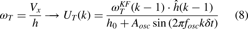

ω_{T} = \frac{V_{x}}{h} ⟶ U_{T} (k) = \frac{ω_{T}^{K F} (k - 1) \cdot \hat{h} (k - 1)}{h_{0} + A_{o s c} \sin (2 π f_{o s c} k δ t)}

(8)

V_{x} (0) \approx ω_{T}^{K F} (k = 0) \cdot \hat{h} (k = 0)

was initialized at

0.45

m/s. To fuse the three translational optic flow cues

ω_{T_{1}}^{m e a s}

ω_{T_{2}}^{m e a s}

and

ω_{T_{3}}^{m e a s}

, a KF was used (see Figure 3). At each

k^{t h}

step, the KF received as input the current value of the model in the equation (8) and as measurements

ω_{T_{1}}^{m e a s}

ω_{T_{2}}^{m e a s}

and

ω_{T_{3}}^{m e a s}

. See Appendix A for the KF calculations.

Fusion strategy using Rough Prior Knowledge (RPK) of the optic flow variations

Here we investigated how to implement the sensor fusion strategy based on 4 optic flow sensors without any knowledge of the oscillation amplitude $A_{o s c}$ or the average flight height $h_{0}$ , just using the information about the general shape and timing of the oscillations during the trajectory.

For this purpose, we approximated very roughly both the optic flow divergence and the translational optic flow cues in the form of a sinusoidal signal serving as the input to both KFs as follows (see Figure 4):

U_{d i v} (k) = - U_{T} (k) = \sin (2 π f_{o s c} k δ t)

(9)

where the oscillation frequency

f_{o s c}

was taken to be equal to

0.28

Hz. At each

k^{t h}

step, the two KFs received as input the current value of the model in the equation (9) and as measurements the optic flow divergence measurements (

ω_{{d i v}_{x}}^{m e a s}

and

ω_{{d i v}_{y}}^{m e a s}

) and the translational optic flow measurements (

ω_{T_{1}}^{m e a s}

ω_{T_{2}}^{m e a s}

and

ω_{T_{3}}^{m e a s}

), respectively. See Appendix A for the KF calculations.

By using as KF input $U_{T} (k) = - s i n (2 π f_{o s c} k δ t)$ , the fusion strategy takes into account the fact that the variation of the translational optic flow is inversely proportional to the flight height $h$ , since it depends only on the ratio $V_{x} / h$ (see equation (1)). As shown in Figure 4, only a rough approximation of the actual shape and timing is taken into account.

Extended Kalman Filter for the fusion strategy with 4 optic flow sensors

To estimate the drone’s flight height $\hat{h}$ , the EKF used received the following:

input: the acceleration of the drone $a_{z}$ ,

measurement: the local optic flow divergence $ω_{d i v}^{K F}$ filtered by the KF based on the optic flow divergence measurements.

See Appendix B for the EKF calculations.

$\hat{h}$ was used to scale the local translational optic flow $ω_{T}^{K F}$ , which was then integrated to perform the odometry as follows:

{\hat{X}}_{S O F I a} = \int ω_{T}^{K F} \cdot \hat{h} d t

(10)

Indoor experimental flight tests

Indoor experimental setup

Indoor flight tests were performed in the Mediterranean Flight Arena (see Figure 5(a)). The position and orientation used in the hexarotor’s control system were taken from the motion-capture (MoCap) system installed in the flight arena, consisting of 17 motion-capture cameras covering a $6 \times 8 \times 4$ m (lxLxH) volume using a VICON $^{TM}$ system. Datasets including the optic flow measurements were recorded via the Robot Operating System (ROS) and processed with the Matlab/Simulink 2022 software.

Figure 5.

Hexarotor flying in the Mediterranean Flight Arena (a). The same dataset taken at $1518 l u x$ was processed with the No Prior Knowledge (NPK) method (b), the Precise Prior Knowledge (PPK) strategy (c) and the Rough Prior Knowledge (RPK) strategy (d). The local Optic Flow (OF) divergence (in blue) measured with the NPK method had a Signal-to-noise Ratio (SnR) of $5.62$ dB (b.i), while with both the PPK and the RPK strategies the SnR was $6.72$ dB (c and d.i). The local translational optic flow (in red) measured with the NPK method had a SnR of $19.12$ dB (b.ii), $25.74$ dB with the PPK strategy (c.ii) and $25.9$ dB with the RPK strategy (d.ii). The flight height estimates $\hat{h}$ converged within $4 s$ with the ground truth values $h$ given by the MoCap system in all 3 cases (b, c and d.iii). The average percentage error of $\hat{h}$ with respect to $h$ after convergence was $- 9.77 %$ with the NPK method (range: $[- 61.5 %, 65.34 %]$ ) (b.iv), $- 2.16 %$ with the PPK strategy (range: $[- 36.89 %, 34.13 %]$ ) (c.iv) and $- 2.55 %$ with the RPK strategy (range: $[- 36.88 %, 34.25 %]$ ) (d.iv). The final percentage error of the distance traveled estimates ${\hat{X}}_{S O F I a}$ with respect to the ground truth $X_{g t}$ was $- 8.57 %$ with the NPK method (b.v), $- 1.22 %$ with the PPK strategy (c.v) and $- 2.80 %$ with the RPK strategy (d.v).

Indoor experimental results

The sensor fusion strategies based on Precise Prior Knowledge (PPK) and Rough Prior Knowledge (RPK) of the optic flow variations (using 4 optic flow sensors) were compared with the strategy based on No Prior Knowledge (NPK) of the optic flow variations (using 2 optic flow sensors). 7 bouncing circular flight tests over a distance of about $50$ m were performed with the hexarotor under an illuminance of $117$ lux ( $5.36 \cdot 10^{- 6} {W / cm}^{2}$ ) and an illuminance of $1518$ lux ( $2.71 \cdot 10^{- 4} {W / cm}^{2}$ ), amounting to a total number of 14 flight tests. First, the 14 datasets were processed with the NPK method (see Section (5.)). The 14 datasets were then processed using the PPK strategy (see Section (6.1.)) and the RPK strategy (see Section (6.2.)). Supp. video n $^{\circ}$ 1 shows a synchronised video of the odometry results obtained with the RPK fusion strategy for the same flight test processed in Figures 5 and 6. The KF parameters discussed in Appendix A were defined experimentally as $Φ = 10$ , $Γ = 10$ and $H_{k} = 10$ , based on the first dataset recorded under an illuminance of $1518$ lux and used to process all 14 datasets for both PPK and RPK fusion strategies.

Figure 6.

(a) Comparison of the position of the hexarotor on the vertical plane ( $x$ , $z$ ) estimated with the Rough Prior Knowledge (RPK) fusion strategy (dashed line) with the ground truth given by the MoCap system (continuous line). The flight height estimates $\hat{h}$ were plotted on the distance traveled estimates ${\hat{X}}_{S O F I a}$ , while the ground truth $h$ was plotted on $X_{g t}$ . This flight test was performed at an illuminance of $1518$ lux. (b) The final percentage error in the distance traveled estimates ${\hat{X}}_{S O F I a}$ with respect to the ground truth $X_{g t}$ was $- 2.63 %$ .

As shown in Figure 5, the optic flow measurements were processed with the three strategies (NPK, RPK and PPK), taking the same dataset recorded under an illuminance of $1518$ lux. The increase in the Signal-to-noise Ratio (SnR, computed as the square ratio of the root mean square of the signal and the root mean square of its noise) for the local optic flow divergence and the local translational optic flow in the case of the PPK and the RPK strategies in comparison with the NPK method affected the average percentage error of the flight height estimates after convergence (at $4$ s). The average percentage error of the flight height estimates was $- 9.77 %$ with the NPK method, $- 2.16 %$ with the PPK strategy and $- 2.8 %$ with the RPK strategy. Similar results were obtained with all 14 datasets. The SnR of the local translational optic flow measured with the NPK method ranged between $18.08$ dB and $24.79$ dB, between $24.84$ dB and $29.93$ dB with the PPK strategy and between $24.84$ dB and $31.39$ dB with the RPK strategy. The SnR of the local optic flow divergence measured with the NPK method ranged between $5.41$ dB and $5.71$ dB, and between $6.47$ dB and $7.11$ dB with both the PPK and RPK strategies.

The flight height estimates $\hat{h}$ and distance traveled estimates ${\hat{X}}_{S O F I a}$ were used to assess the position of the hexarotor on the vertical plane ( $x$ , $z$ ). An example is shown in Figure 6, where the flight height estimates $\hat{h}$ were plotted on the distance traveled estimates ${\hat{X}}_{S O F I a}$ (which are given directly in meters) and compared with the ground truth values given by the MoCap system. Since the 2D position estimates were based on the optic flow based odometry, they were subject to an accumulated error increasing with the distance covered.

Overall, the final percentage error in the distance traveled estimates ${\hat{X}}_{S O F I a}$ with respect to the ground truth $X_{g t}$ (traveled along the $x$ axis) ranged between $- 8.57 %$ and $8.4 %$ with the NPK method, between $- 4.02 %$ and $2.38 %$ with the PPK strategy and between $- 4.65 %$ and $2 %$ with the RPK strategy (see Figure 7(b)). Similar results were obtained taking the two different illuminances separately (see Figure 7(a)).

Figure 7.

Distributions of the final percentage errors in the distance traveled estimates ${\hat{X}}_{S O F I a}$ with respect to the ground truth $X_{g t}$ (traveled along the $x$ axis) for 7 datasets recorded at $1518$ lux and 7 datasets recorded at $117$ lux. a.i) At an illuminance of $1518 l u x$ , the final percentage error ranged between $- 8.57 %$ and $5.52 %$ (with a median value of $- 1.14 %$ ) in the case of the No Prior Knowledge (NPK) method (in black), between $- 1.65 %$ and $1.08 %$ (with a median value of $- 0.8 %$ ) in that of the Precise Prior Knowledge (PPK) strategy (in purple) and between $- 3.95 %$ and $0.63 %$ (with a median of $- 1.55 %$ ) in that of the Rough Prior Knowledge (RPK) strategy (in green). a.ii) At an illuminance of $117 l u x$ , the final percentage error ranged between $- 0.72 %$ and $8.4 %$ (with a median value of $4.73 %$ ) with the NPK method, between $- 4.02 %$ and $2.38 %$ (with a median of $- 0.27 %$ ) with the PPK strategy and between $- 4.65 % %$ and $2 %$ (with a median value of $- 1.14 %$ ) with the RPK strategy. b) Upon combining all 14 datasets recorded, the final percentage error ranged between $- 8.57 %$ and $8.4 %$ (median value: $0.47 %$ ) with the NPK method, between $- 4.02 %$ and $2.38 %$ (median value: $- 0.53 %$ ) with the PPK strategy and between $- 4.65 %$ and $2 %$ (median value: $- 1.34 %$ ) with the RPK strategy.

Preliminary outdoor experimental flight tests

Outdoor experimental setup

Outdoors, for trajectory tracking purposes, the hexarotor was equipped with a TeraRanger Evo 3m distance sensor in order to measure the flight height of the drone and with a Pixhawk GPS sensor (from Holybro) in order to measure the horizontal position. These 2 sensors were connected directly to the PX4 flight controller. In order to validate the precision of the TeraRanger Evo 3m distance sensor with the help of the MoCap system, a test was performed in the flight arena, in which we observed that TeraRanger Evo 3m was very reliable. This reliability was confirmed by the quality of the TeraRanger Evo 3m sensor’s output, which was devoid of high frequency noise when measured on the field (see Section (2.) of Supp. Information). According to the PX4 documentation, the standard deviation of the horizontal position error is $0.8$ m using GPS outdoors. We observed that the hexarotor flying in the horizontal plane had a maximum deviation of about $1$ m with respect to the desired trajectory (see Figure 8). Besides, the physical distance on the hexarotor of $5$ cm between the TeraRanger Evo 3m sensor and the optic flow sensors has been subtracted to the flight height estimates $\hat{h}$ to be compared to the ground truth $h$ (measured by the TeraRanger Evo 3m sensor) in Figures 9, 10 and 11.

Figure 8.

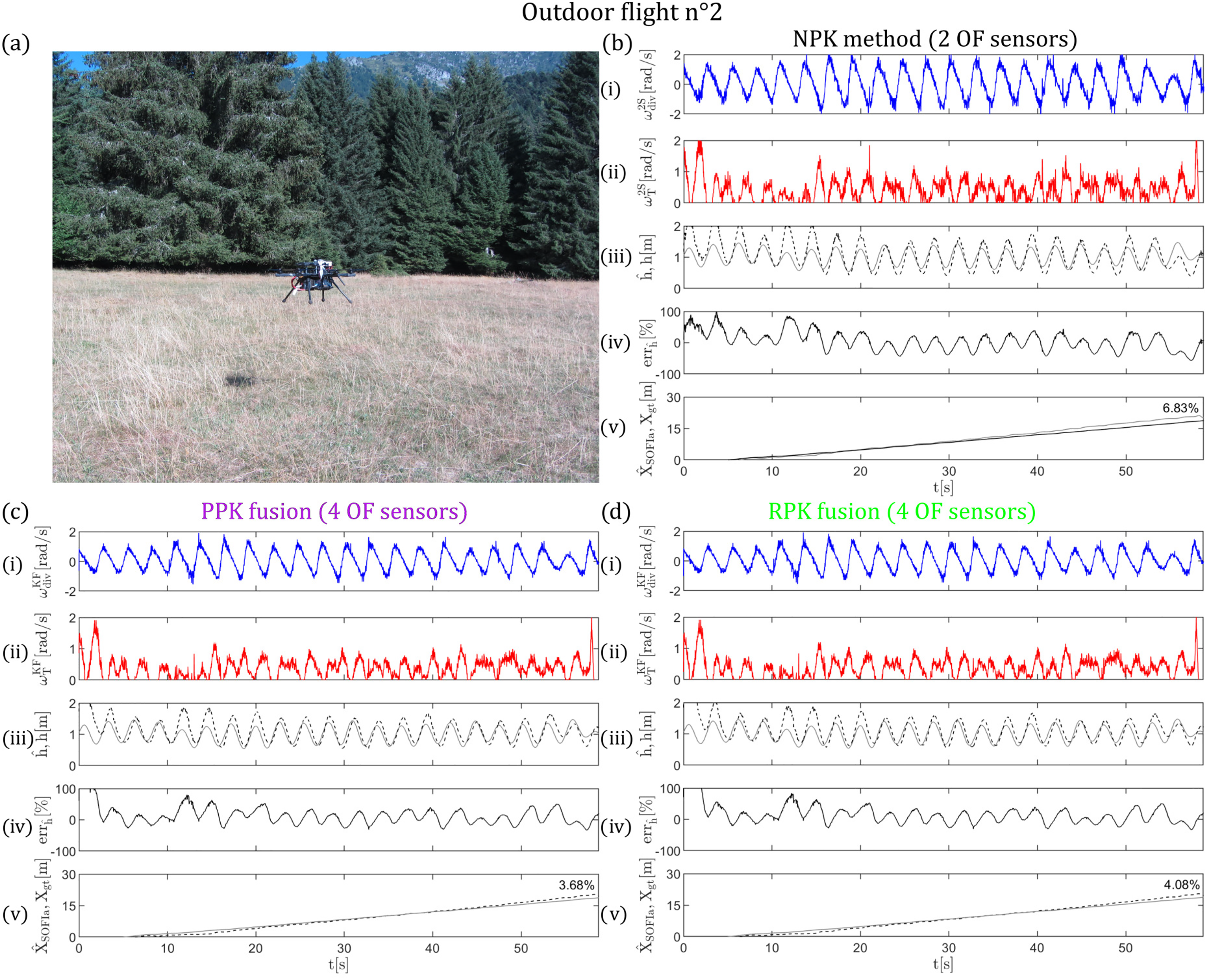
Top view of the drone’s horizontal trajectory during an outdoor flight test (outdoor flight n $^{\circ}$ 2). The drone was equipped with a TeraRanger Evo 3m distance sensor to measure the flight height and a Pixhawk GPS to measure its position on the horizontal plane ( $x$ , $y$ ). The take-off point of the flight was taken to be $[0, 0]$ . The optic flow based odometry is performed along the darker part of the trajectory.

Figure 9.

Hexarotor flying over a field irregularly covered with grass (outdoor flight n $^{\circ}$ 2) (a). The same dataset recorded outdoors was processed with the No Prior Knowledge (NPK) method (b), the Precise Prior Knowledge (PPK) strategy (c) and the Rough Prior Knowledge (RPK) strategy (d). The local Optic Flow (OF) divergence (in blue) measured had a Signal-to-noise Ratio (SnR) of $5.74$ dB with the NPK method (b.i), $6.15$ dB with the PPK strategy (c.i) and $6.14$ dB with the RPK strategy (d.i). The local translational optic flow (in red) measured had a SnR of $5.9$ dB with the NPK method (b.ii), $7.41$ dB with the PPK strategy (c.ii) and $7.4$ dB with the RPK strategy (d.ii). The flight height estimates $\hat{h}$ converged within $5 s$ with the ground truth values $h$ given by the distance sensor in all 3 cases (b, c and d.iii). The average percentage error of $\hat{h}$ with respect to $h$ after convergence was $1.1 %$ with the NPK method (range: $[- 56.77 %, 85.65 %]$ ) (b.iv), $7.12 %$ with the PPK strategy (range: $[- 33.91 %, 79.94 %]$ ) (c.iv) and $7.19 %$ with the RPK strategy (range: $[- 33.91 %, 83.34 %]$ ) (d.iv). The distance traveled estimates ${\hat{X}}_{S O F I a}$ with respect to the ground truth $X_{g t}$ were computed only after convergence. The final percentage error was $6.83 %$ with the NPK method (b.v), $3.68 %$ with the PPK strategy (c.v) and $4.08 %$ with the RPK strategy (d.v).

Figure 10.

(a) Comparison between the position of the hexarotor on the vertical plane ( $x$ , $z$ ) estimated with the Rough Prior Knowledge (RPK) fusion strategy (dashed line) and the ground truth values given by the distance sensor (continuous line) (outdoor flight n $^{\circ}$ 2). The flight height estimates $\hat{h}$ were plotted on the distance traveled estimates ${\hat{X}}_{S O F I a}$ , while $h$ was plotted on $X_{g t}$ (the ground truth values). (b) The final percentage error in the distance traveled estimates ${\hat{X}}_{S O F I a}$ with respect to the ground truth values $X_{g t}$ was $4.08 %$ .

Figure 11.

In the 4 datasets recorded outdoors, the final percentage error in the distance traveled estimates ${\hat{X}}_{S O F I a}$ with respect to the ground truth values $X_{g t}$ ranged between $1.77 %$ and $17.23 %$ (median value: $4.67 %$ ) with the No Prior Knowledge (NPK) method (in black), between $- 8.92 %$ and $9.4 %$ (median value: $- 2.49 %$ ) with the Precise Prior Knowledge (PPK) strategy (in purple) and between $- 8.37 %$ and $9.7 %$ (median value: $- 2.1 %$ ) for Rough Prior Knowledge (RPK) (in green).

The outdoor experiments were performed using the same set of Pixart PAW3903 optic flow sensors, but adding a neutral density filter of 2 in front of the lenses to attenuate the solar luminosity. Without these filters, the optic flow sensors would have been saturated.

Results of preliminary outdoor experiments

4 bouncing longitudinal flight tests over a distance of about $20 m$ were performed with the hexarotor outdoors over a field irregularly covered with grass (see Supp. video n $^{\circ}$ 2 and 3). In Figure 9, the optic flow measurements of the outdoor flight number 2 were processed with the NPK method, the PPK strategy and the RPK strategy (see the odometry results obtained with the RPK fusion strategy in Supp. video n $^{\circ}$ 2 for the outdoor flight number 2). The values of the KF parameters defined in Appendix A were those previously used in the indoor flight tests. As with the indoor flight tests, the SnRs of the local optic flow divergence and those of the local translational optic flow were greater with the PPK and RPK strategies than with the NPK method (see Section (1.) of Supp. Information). Figure 10 gives the 2D position estimation on the vertical plane ( $x$ , $z$ ) for the outdoor flight number 2.

Due to the presence of wind disturbances and the greater convergence time required by the EKF in outdoor visual setting, the distance traveled ${\hat{X}}_{S O F I a}$ was estimated only after a convergence time of $5 s$ . Overall, the final percentage error in the distance traveled estimates ${\hat{X}}_{S O F I a}$ with respect to the ground truth values $X_{g t}$ ranged between $1.77 %$ and $17.23 %$ with the NPK method, between $- 8.92 %$ and $9.4 %$ with the PPK strategy and between $- 8.37 %$ and $9.7 %$ with the RPK strategy (see Figure 11). As with the indoor flights (see Figure 7), Figure 11 shows comparable results between the PPK and the RPK fusion strategies. The RPK fusion strategy seems to be very interesting because it only uses knowledge of the timing and general shape of the translational and divergence optic flow cues. This knowledge can be considered reasonable since it is available onboard the UAV: it is in fact the drone itself that shapes the optic flow cues by creating these oscillations.

Conclusion

In this study, we investigated how to use information about the oscillating trajectory to improve a minimalistic odometry based on optic flow cues. The experiments were performed onboard a hexarotor first indoors, following circular bouncing trajectories at a frequency of $0.28$ Hz over distances of about $50$ m under illuminances of $117$ lux and $1518$ lux. The results were not affected by the illuminance conditions. A few tests were then performed outdoors, where the hexarotor followed bouncing longitudinal trajectories over a distance of about $20$ m over a field irregularly covered with grass in the presence of various wind conditions.

The findings obtained in this study show that the sensor fusion strategies based on the use of 4 optic flow sensors make it possible to measure the optic flow divergence and the translational optic flow cues more reliably thanks to the use of additional Kalman Filters. This was the case even when taking only rough prior knowledge about the optic flow variations into account, and more specifically, only the general shape and timing of the oscillations during the trajectory. This prior knowledge can be considered acceptable since the general shape and timing of the oscillations are imposed by the drone itself on its own forward trajectory. The sensor fusion strategies presented decreased the error in the flight height estimates, and thus decreased the percentage error in the distance traveled estimates in all the cases considered, improving the odometric performances. These considerations also applied in the case of the few outdoor flight tests performed in the presence of wind and an irregular pattern of grass.

With all three odometric processing methods, the final distance traveled estimates were admittedly subject to small errors as the odometric strategy is a dead reckoning method involving no feedback from the environment. Nevertheless, we show here that the SOFIa model can be accurate and precise enough to move in close proximity to a target without GPS, indoors and outdoors. Likewise, this highly minimalistic optic flow based odometric strategy could also be used to enable a future drone to assess whether it is returning near its base station without any need for a GPS. So far, the present findings can be said to constitute the first experimental proof-of-concept of the SOFIa model²⁶ before this optic flow based odometric strategy is implemented on a nanodrone requiring very little computational power.³⁰ We now intend to test the robustness of these strategies in a range of forward speeds, in cases where a large drone pitch occurs and in the presence of strong reliefs.

Future studies will also include the implementation of an optic flow regulator keeping the translational optic flow around a given setpoint.

Supplemental Material

sj-pdf-1-mav-10.1177_17568293221148380 - Supplemental material for Indoor and outdoor in-flight odometry based solely on optic flows with oscillatory trajectories

Supplemental material, sj-pdf-1-mav-10.1177_17568293221148380 for Indoor and outdoor in-flight odometry based solely on optic flows with oscillatory trajectories by L Bergantin, C Coquet, J Dumon, A Negre, T Raharijaona, N Marchand and F Ruffier in International Journal of Micro Air Vehicles

Footnotes

Acknowledgements

We thank Dr. J. Blanc for improving the English manuscript and J.M. Ingargiola for his help with designing the printed circuit boards for the optic flow sensors. We are grateful to the three anonymous Referees, whose suggestions have helped us to greatly improve the manuscript.

Declaration of conflicting interests

The author(s) declared no potential conflicts of interest with respect to the research, authorship, and/or publication of this article.

Funding

The author(s) disclosed receipt of the following financial support for the research, authorship, and/or publication of this article: Financial support was provided via a ProxiLearn project grant (ANR-19-ASTR-0009) to F.R. from the ANR (Astrid Program). The participation of L.B. in this research project was supported by a joint PhD grant from the Délégation Générale de l'Armement (DGA) and Aix Marseille University. The participation of C.C. was also supported by the CNRS Innovation via a pre-maturation project. L.B, C.C., and F.R. were also supported by Aix Marseille University and the CNRS (Life Science, Information Science Institute as well as Engineering Science & Technology Institute). The equipments for the experimental tests have been mainly supported by ROBOTEX 2.0 (Grants ROBOTEX ANR-10-EQPX-44-01 and TIRREX ANR-21-ESRE-0015).

ORCID iDs

L Bergantin

A Negre

Supplemental material

Supplementary material for this article is available online.

Notes

Appendix A: Kalman Filter calculations

In the PPK strategy, the optic flow divergence and the translational optic flow cues were expressed as in the equations (7) and (8), respectively. In the RPK strategy, the optic flow divergence and the translational optic flow cues were both expressed as in the equation (9). With each optic flow cue, at each $k^{t h}$ step, the current value of the corresponding model was computed and given to the corresponding KF as input (see Figure 3). In the following paragraph, the notation $A > 0$ indicates a strictly positive definite matrix. The KF took the following iterative steps at each $k^{t h}$ time:

Prediction step

(a) One-step ahead prediction (11)

X_{k / k - 1} = Φ \cdot X_{k - 1 / k - 1} + Γ \cdot U_{k - 1 / k - 1}

with

Φ > 0, Γ > 0

(b) Covariance matrix of the state prediction error vector (12)

P_{k / k - 1} = Φ \cdot P_{k - 1 / k - 1} \cdot Φ^{T} + Q

Correction step

X_{k / k} = X_{k / k - 1} + K_{k} \cdot (Y_{k}^{i} - H_{k} \cdot X_{k / k - 1})

with

Y_{k}^{i}

current value of the

i^{t h}

measurement,

H_{k} > 0

and

K_{k}

Kalman gain defined as: (14)

K_{k} = P_{k / k - 1} \cdot H_{k}^{T} \cdot [H_{k} \cdot P_{k / k - 1} \cdot H_{k}^{T} + R_{k}]^{- 1}

The measurement update step was repeated for each

i^{t h}

measurement (2 times for the optic flow divergence and 3 times for the translational optic flow).

(d) Covariance matrix of state estimation error vector (15)

P_{k / k} = P_{k / k - 1} + K_{k} \cdot [H_{k} \cdot P_{k / k - 1} \cdot H_{k}^{T} + R_{k}] \cdot K_{k}^{T}

(e) Innovation (16)

{\tilde{Y}}_{k} = Y_{k} - H_{k} \cdot X_{k / k}

Appendix B: Extended Kalman Filter calculations

The discretized model for the hexarotor along the vertical axis (see equation (6)) can be expressed as follows: (17)

{\begin{matrix} X [k + 1] = Φ \cdot X [k] + Γ \cdot U [k] \\ Y [k] = C_{k} \cdot X [k] + D_{k} \cdot U [k] \end{matrix}

with (18)

Φ = e^{A \cdot d t}

(19)

Γ = (\int_{0}^{d t} e^{A \cdot τ} d τ) \cdot B = (A^{T} \cdot e^{A \cdot d t} - A^{T}) \cdot B

(20)

C_{k} = g (X_{k}) = [\frac{X_{2} [k]}{X_{1} [k]}] = [\frac{V_{h} [k]}{h [k]}]

(21)

D_{k} = 0

where

d t

is the discretization time. To estimate the flight height

h

, the EKF took the following iterative steps at each

k^{t h}

time:

Prediction step

(a) One-step ahead prediction (22)

X_{k / k - 1} = Φ \cdot X_{k - 1 / k - 1} + Γ \cdot U_{k - 1 / k - 1}

(b) Covariance matrix of the state prediction error vector (23)

P_{k / k - 1} = Φ \cdot P_{k - 1 / k - 1} \cdot Φ^{T} + Q

Correction step

X_{k / k} = X_{k / k - 1} + K_{k} \cdot (Y_{k} - H_{k} \cdot X_{k / k - 1})

with

K_{k}

Kalman gain defined as: (25)

K_{k} = P_{k / k - 1} \cdot H_{k}^{T} \cdot [H_{k} \cdot P_{k / k - 1} \cdot H_{k}^{T} + R_{k}]^{- 1}

and

H_{k}

Jacobian matrix for the non linear function defined as follows: (26)

H_{k} = \frac{\partial g}{\partial X} |_{X = X_{k / k - 1}} = [\begin{matrix} - \frac{V_{h}}{h^{2}} & \frac{1}{h} \end{matrix}]

(d) Covariance matrix of state estimation error vector (27)

P_{k / k} = P_{k / k - 1} + K_{k} \cdot [H_{k} \cdot P_{k / k - 1} \cdot H_{k}^{T} + R_{k}] \cdot K_{k}^{T}

(e) Innovation (28)

{\tilde{Y}}_{k} = Y_{k} - H_{k} \cdot X_{k / k}

Appendix C: Computation of the local divergence and translational optic flow cues

The local optic flow divergence can be measured as the difference between two optic flow magnitudes $ω (ϕ)$ and $ω (- ϕ)$ perceived by two optic flow sensors oriented at angles $\pm ϕ$ with respect to the normal to a surface, divided by a known factor of $\sin 2 ϕ$ : (29)

ω_{d i v}^{m e a s} = \frac{ω (ϕ) - ω (- ϕ)}{\sin 2 ϕ} = \frac{V_{h}}{h}

The local translational optic flow can be measured as the sum of

ω (ϕ)

and

ω (- ϕ)

, divided by a known factor of

2 \cdot \cos^{2} ϕ

: (30)

ω_{T}^{m e a s} = \frac{ω (ϕ) + ω (- ϕ)}{2 \cdot \cos^{2} ϕ} = \frac{V_{x}}{h}

References

Strydom

Thurrowgood

Srinivasan

. Visual odometry: autonomous uav navigation using optic flow and stereo. In Proceedings of Australasian conference on robotics and automation.

Kumar

Kaingade

et al. Visual odometry using optic flow for unmanned aerial vehicles. In 2015 International Conference on Cognitive Computing and Information Processing(CCIP). pp. 1–6. doi:10.1109/CCIP.2015.7100731.

Vidal

Rebecq

Horstschaefer

et al. Ultimate slam? combining events, images, and imu for robust visual slam in hdr and high-speed scenarios. IEEE Robot Autom Lett 2018; 3: 994–1001.

Denuelle

Srinivasan

. A sparse snapshot-based navigation strategy for uas guidance in natural environments. In 2016 IEEE International Conference on Robotics and Automation (ICRA). IEEE, pp. 3455–3462.

Kendoul

Fantoni

Nonami

. Optic flow-based vision system for autonomous 3d localization and control of small aerial vehicles. Rob Auton Syst 2009; 57: 591–602.

Faessler

Fontana

Forster

et al. Autonomous, vision-based flight and live dense 3d mapping with a quadrotor micro aerial vehicle. Journal of Field Robotics 2016; 33: 431–450.

de Croon

Lee

. Stability-based scale estimation for monocular slam. IEEE Robotics and Automation Letters 2018; 3: 780–787.

Milijas

Markovic

Ivanovic

et al. A comparison of lidar-based slam systems for control of unmanned aerial vehicles. In 2021 International Conference on Unmanned Aircraft Systems (ICUAS). IEEE, pp. 1148–1154.

Shurin

Klein

. Qdr: A quadrotor dead reckoning framework. IEEE Access 2020; 8: 204433–204440.

10.

Ruffier

Franceschini

. Optic flow regulation: the key to aircraft automatic guidance. Rob Auton Syst 2005; 50: 177–194.

11.

Expert

Ruffier

. Flying over uneven moving terrain based on optic-flow cues without any need for reference frames or accelerometers. Bioinspir Biomim 2015; 10. DOI: 10.1088/1748-3190/10/2/026003.

12.

Iida

. Biologically inspired visual odometer for navigation of a flying robot. Rob Auton Syst 2003; 44: 201–208.

13.

Kendoul

Fantoni

Nonami

. Optic flow-based vision system for autonomous 3d localization and control of small aerial vehicles. Rob Auton Syst 2009; 57: 591–602.

14.

Serres

Ruffier

. Optic flow-based collision-free strategies: From insects to robots. Arthropod Struct Dev 2017; 46: 703–717.

15.

Kirchner

Srinivasan

. Freely flying honeybees use image motion to estimate object distance. Naturwissenschaften 1989; 76: 281–282.

16.

Serres

Masson

Ruffier

et al. A bee in the corridor: centering and wall-following. Naturwissenschaften 2008; 95: 1181–1187.

17.

Portelli

Ruffier

Roubieu

et al. Honeybees’ speed depends on dorsal as well as lateral, ventral and frontal optic flows. PLoS ONE 2011; 6: e19486.

18.

Portelli

Ruffier

Franceschini

. Honeybees change their height to restore their optic flow. J Comp Physiol A 2010; 196: 307–313.

19.

Portelli

Serres

Ruffier

. Altitude control in honeybees: joint vision-based learning and guidance. Sci Rep 2017; 7: 1–10.

20.

Herissé

Hamel

Mahony

et al. Landing a vtol unmanned aerial vehicle on a moving platform using optical flow. IEEE Trans Robot 2011; 28: 77–89.

21.

Van Breugel

Morgansen

Dickinson

. Monocular distance estimation from optic flow during active landing maneuvers. Bioinspir Biomim 2014; 9: 025002.

22.

de Croon

. Monocular distance estimation with optical flow maneuvers and efference copies: a stability-based strategy. Bioinspir Biomim 2016; 11: 016004.

23.

de Croon

Chu

. Distance and velocity estimation using optical flow from a monocular camera. Int J Micro Air Vehicles 2017; 9: 198–208.

24.

Creuze

. Monocular odometry for underwater vehicles with online estimation of the scale factor. In IFAC 2017 World Congress.

25.

Bergantin

Raharijaona

Ruffier

. Estimation of the distance from a surface based on local optic flow divergence. In 2021 International Conference on Unmanned Aircraft Systems (ICUAS). IEEE, pp. 1291–1298.

26.

Bergantin

Harbaoui

Raharijaona

et al. Oscillations make a self-scaled model for honeybees’ visual odometer reliable regardless of flight trajectory. J R Soc Interface 2021; 18: 20210567.

27.

Bergantin

Coquet

Negre

et al. Minimalistic in-flight odometry based on two optic flow sensors along a bouncing trajectory. In IEEE International Conference on Control, Automation and Systems (ICCAS). Busan, South Korea.

28.

Meier

Honegger

Pollefeys

. Px4: A node-based multithreaded open source robotics framework for deeply embedded platforms. In 2015 IEEE International Conference on Robotics and Automation (ICRA). pp. 6235–6240. DOI:10.1109/ICRA.2015.7140074.

29.

Gibson

. The perception of the visual world. Boston: Houghton Mifflin, 1950.

30.

Palossi

Marongiu

Benini

. Ultra low-power visual odometry for nano-scale unmanned aerial vehicles. In Design, Automation Test in Europe Conference Exhibition (DATE), 2017. pp. 1647–1650. DOI:10.23919/DATE.2017.7927257.

Supplementary Material

Please find the following supplemental material available below.

For Open Access articles published under a Creative Commons License, all supplemental material carries the same license as the article it is associated with.

For non-Open Access articles published, all supplemental material carries a non-exclusive license, and permission requests for re-use of supplemental material or any part of supplemental material shall be sent directly to the copyright owner as specified in the copyright notice associated with the article.

0.00 MB

1.82 MB