Low order modeling of dynamic stall using vortex particle method and dynamic mode decomposition

Abstract

Low order modelings are performed in this paper, including iterative Brinkman penalized vortex method (IBVM) and data-driven dynamic mode decomposition (DMD) for dynamic stall study of symmetric airfoil. The data are extracted from IBVM as input for flow field reconstruction using combinations of DMD dominant modes, representing extracted flow features. The primary mode together with its harmonics, and the mean mode are termed to be dominant for the airfoil wake duplication at fixed angles of attack ( $\alpha$ ) ranging from ${20}^{\circ }$ to ${90}^{\circ }$ . For the dynamic stall duplication, at small and large pitching amplitudes, the nearfield and farfield vorticty contours from the DMD generally agree well with those from the IBVM. In addition, the lift coefficient from the DMD collapses well with that from the IBVM and the experiment.

Introduction

The dynamic stall is the classical phenomenon resulting in a dramatic loss of lift coefficient because of the non-quasi-steady pitching motion of slender bodies in unsteady flow. Although the dynamic stall was early documented by Kramer, ¹ it is still an interesting topic among aerodynamicists due to its massive effects on aerodynamic and structural performance. These effects were observed by a series of research leading to challenging applications, including helicopter rotor blades,^2–5 highly maneuverable fixed-wing aircrafts, ⁶ wind turbines,^7–9 compressor,^10–14 flapping wings,^15–21 and laminar separation flutter.^22–24 Figure 1 shows an illustration of static and dynamic stall over an airfoil surface at an angle of attack ranging from small to high values. As shown in Figure 1(a), the boundary layer attaches to the upper surface of an airfoil; and the separation point appears near the trailing edge. When the angle of attack increases, depicted in Figure 1(b), the separation point moves to the leading edge due to an adverse pressure gradient, forming the leading edge vortex that attaches to the airfoil surface. The leading edge vortex enlarges its size as the adverse pressure gradient is intensified; and this vortex tends to detach from the surface as its size reaches its maximum with an increase in the angle of attack, as shown in Figure 1(c). Simultaneously, the trailing edge vortex develops its size and finally sheds downstream. As the angle of attack is sufficiently high, the counterrotating leading and trailing edge vortices shed downstream; and their nonlinear interactions form the Karman vortex street with low frequency, as shown in Figure 1(d). At a sufficiently high Reynolds number (based on airfoil chord length), the Kelvin-Helmholtz vortex occurs with high frequency as a result of the instability of the shear layer shed from the leading and trailing edges of the airfoil. It can be concluded that the dynamic stall around an airfoil is quite complex where the various coherent structures (Karman and Kelvin-Helmholtz vortices) are formed due to the nonlinear interactions of the shear layers and the boundary layers. The analysis of this complex flow aims to extract the physically significant features, denoted as modes, as a first step in the analysis. For this purpose, low-order modeling methods are required to resolve these modes that represent these different time scales or frequencies.

Figure 1.

Illustration of static and dynamic stall over an airfoil surface at angle of attack ranging from small to high values. (a): attached boundary layer at quasi-steady mode. (b): development of leading edge vortex at quasi-steady mode. (c): development of leading and trailing edge votices at quasi-steady mode. (d): stall at dynamic mode with the occurence of Kelvin-Helmholtz vortex (high frequency) and Karman vortex (low frequency).

Otherwise, computational fluid dynamic (CFD) models are generally based on variables located in spatial and temporal coordinates. The spatial computational domains for resolving the dynamic stall are discretized into up to ${10}^6$ grid nodes to obtain sufficient accuracy.^25,26 Therefore, CFD models are high order, requiring considerably computational cost. In addition, the major issue of large-scale complex flow modeling is the reduction of the computational cost while preserving numerical accuracy. Hence, low-order modeling necessitates transforming the high-fidelity model onto a reduced space basis. Based on the reduced space basis, the Navier-Stokes equations are transformed into a set of ordinary differential equations in time, requiring a greatly reduced computational effort. The low order modelings are classified into the vortex method, ²⁷ Galerkin projection, ²⁸ and dynamic mode decomposition (DMD). ²⁹ While the vortex method and Galerkin projection transform infinite-dimensional Navier-Stokes equations into a finite set of ordinary differential equations, DMD is a data-driven technique. For the bluff and slender body applications, various studies of vortex methods have been reported.^{30–33,22,34} In addition, the wake dynamics of those has been studied by many authors using DMD, where spatially varying coherent structures and their frequencies are obtained.^35–40 In this paper, two low-order techniques, namely, dynamic mode decomposition (DMD) and the iterative Brinkman penalized vortex particle method (IBVM), ³² are employed. The IBVM is employed to extract the fully dominant coherent structures present in the flow, and these structures may contain multiple frequencies. Using DMD, a single characteristic frequency contained in each coherent structure is obtained separately. Based on these frequencies, the flow field is reconstructed to study the spatial behavior of the different frequency components.

In the present paper, flow past a symmetric airfoil is studied for three fixed angles of attack ( $\alpha ={20}^{\circ },{60}^{\circ }$ , and ${90}^{\circ }$ ) at a constant value of Re = 1000. Then, the dynamic stall of a pitching symmetric airfoil is also investigated at Re = 4000. Based on the work of Kurtulus, ⁴¹ the Reynolds number of 1000 is sufficient for the occurrence of small-scale (Kelvin-Helmholtz) and large-scale (Karman) vortices behind the airfoil. The data for DMD is obtained using direct numerical simulations (IBVM). The problem statement and formulation of IBVM and DMD are presented in Sections ‘Iterative Brinkman penalized vortex method’ and ‘Dynamic mode decomposition’, respectively. Validations are provided in Section ‘Computation setup’. The results and discussion are presented in Section ‘Results and discussion’ and the conclusions are provided in Section ‘Conclusions’.

Iterative Brinkman penalized vortex method

In this work, the iterative Brinkman penalized vortex method (IBVM) proposed by Duong and Lavi ³² is employed to simulate the two-dimensional incompressible flow over a sharp-shape body. For a brief introduction of the IBVM, the Navier-Stokes equations in pressure-velocity form for incompressible flows are initially described as follows.

$$\mathbf{\nabla }\cdot \mathit{u}=0,\mathit{x}\in \mathrm{\Xi }$$

(1)

$$\frac{\mathrm{\partial }\mathit{u}}{\mathrm{\partial }t}+\mathit{u}\cdot \mathbf{\nabla }\mathit{u}=-\frac{1}{\rho }\mathbf{\nabla }p+\nu {\mathbf{\nabla }}^2\mathit{u},\mathit{x}\in \mathrm{\Xi }$$

(2)

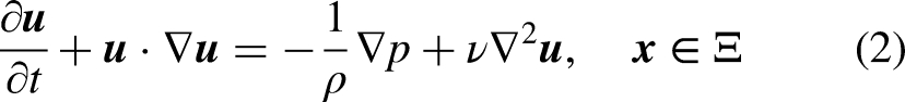
where $\mathrm{\Xi }$ stands for the fluid domain, $\mathit{u}$ , $\rho$ , $p$ and $\nu$ are the velocity field, the fluid density, pressure, and kinematic viscosity, respectively. $\mathit{x}$ and $t$ represent spatial and time domains, respectively. Taking the curl of the equations (1) and (2), and using the vector identity ( $\mathit{\omega }=\mathbf{\nabla }\times \mathit{u}$ and $\mathbf{\nabla }\cdot \mathit{\omega }=0$ ), these equations become the following equations.

$$\mathbf{\nabla }\cdot \mathit{\omega }=0,\mathit{x}\in \mathrm{\Xi }$$

(3)

$$\frac{\mathrm{\partial }\mathit{\omega }}{\mathrm{\partial }t}+\mathit{u}\cdot \mathbf{\nabla }\mathit{\omega }=\mathit{\omega }\cdot \mathbf{\nabla }\mathit{u}+\nu {\mathbf{\nabla }}^2\mathit{\omega },\mathit{x}\in \mathrm{\Xi }$$

(4)

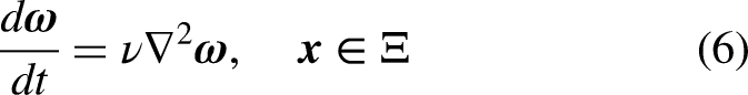
These equations are expressed as the velocity( $\mathit{u}$ )-vorticity( $\mathit{\omega }$ ) formulation, where the pressure term is neglected because $p$ is scalar. In incompressible two-dimensional flows, the vortex stretching ( $\mathit{\omega }\cdot \mathbf{\nabla }\mathit{u}$ ) and the divergence ( $\mathbf{\nabla }\cdot \mathit{\omega }$ ) are neglected. Hence, the equations (3) and (4) are expressed in Lagrangian description as

$$\frac{d\mathit{x}}{dt}=\mathit{u}(\mathit{x},t),\mathit{x}\in \mathrm{\Xi }$$

(5)

$$\frac{d\mathit{\omega }}{dt}=\nu {\mathbf{\nabla }}^2\mathit{\omega },\mathit{x}\in \mathrm{\Xi }$$

(6)

where the right-hand side of the equation (6) is the diffusion term. The new position and vorticity of particles are updated by solving the equations (5) and (6) using the fourth-order Runge–Kutta method performed by Duong et al.,^31,34,33 where the velocity field on the right-hand side of equation (5) is computed by the Biot-Savart formulation^42,43:

$${\mathit{u}}_i=\frac{1}{4\pi }\sum _{j=1}^N\frac{{\mathbf{\Gamma }}_j\times ({\mathit{x}}_i-{\mathit{x}}_j)}{{\sigma }^2{|{\mathit{x}}_i-{\mathit{x}}_j|}^2}+{\mathit{U}}_0$$

(7)

where $\mathbf{\Gamma }={\int }_V\mathit{\omega }\mathrm{d}\mathrm{V}$ is the particle strength; $i$ and $j$ stand for the $i^{th}$ and $j^{th}$ particles and $\sigma$ is the particle core size. Since the Biot-Savart formulation requires $O(N^2)$ operations, the fast multipole method is utilized to reduce the computational cost from $O(N^2)$ to $O(N\log N)$ .

In order to descritize the diffusion term on the right-hand side of the equation (6), the particle strength exchange method^44,45 is used as:

$${\int }_V\left({\mathbf{\nabla }}^2\mathit{\omega }\right)\mathrm{d}\mathrm{V}=2\nu \sum _{\mathrm{j}=1}^{\mathrm{N}}\frac{1}{{\sigma }_{\mathrm{ij}}^2}{\mathrm{G}}_{\sigma }(|{\mathit{x}}_{\mathrm{i}}-{\mathit{x}}_{\mathrm{j}}|)({\sigma }_{\mathrm{i}}^2{\mathbf{\Gamma }}_{\mathrm{j}}-{\sigma }_{\mathrm{j}}^2{\mathbf{\Gamma }}_{\mathrm{i}})$$

(8)

where $G_{\sigma }=\frac{1}{2\pi {\sigma }^2}\exp (-\frac{|\mathit{x}{|}^2}{2{\sigma }^2})$ is the Gaussian smoothing kernel expressing particle distribution. The solutions of the equations (5) and (6) induce the particle distortion issue due to the Lagrangian effect. Hence, the $M_4^{\prime }$ remeshing scheme is employed to deal with the issue

$$M_4^{\prime }\left(x\right)=\{\begin{array}{cc}1-\frac{5{\left|x\right|}^2}{2}+\frac{3{\left|x\right|}^3}{2},& \mathrm{if}0\le \left|\mathrm{x}\right|\le 1\\ \frac{1}{2}{(2-\left|x\right|)}^2(1-\left|x\right|),& \mathrm{if}1\le \left|\mathrm{x}\right|\le 2\\ 0,& \mathrm{if}\left|\mathrm{x}\right|>2\end{array}$$

(9)

To deal with the bounded-flow simulation, the iterative Brinkman penalization is used. The penalization term can be expressed in the vorticity formulation as

$$\frac{\mathrm{\partial }\mathit{\omega }}{\mathrm{\partial }t}=\mathbf{▽}\times \left[\lambda \chi ({\mathit{u}}_s-\mathit{u})\right]$$

(10)

where ${\mathit{u}}_s$ denotes the velocity of the body and $\mathit{u}$ denotes the velocity field of the flow; the penalization parameter $\lambda$ is chosen to be $\lambda =\frac{1}{△t}$ ; $\chi$ is the characteristic function

$$\chi =\{\begin{array}{cc}0,& \mathrm{if}\mathrm{r}<-ϵ\\ \frac{1}{2}[1+\frac{r}{ϵ}+\frac{1}{\pi }\sin \left(\pi \frac{r}{ϵ}\right)],& \mathrm{if}\left|\mathrm{r}\right|\le ϵ\\ 1,& \mathrm{if}\mathrm{r}>ϵ\end{array}$$

(11)

In the penalized domain, the computed velocity by the Biot-Savart formulation ( $\tilde{\mathit{u}}$ ) is deviated from the imposed velocity in the body ( ${\mathit{u}}_s$ ). Therefore, the iterative penalization method simply alters the second term of the right hand side of the equation (10), introducing penalization velocity, ${\mathit{u}}_{\omega }$ , as follows

$$△{\mathit{\omega }}^k=\mathbf{\nabla }\times [\chi ({\mathit{u}}_s-\tilde{\mathit{u}}-{\mathit{u}}_{\omega }^{k-1})]$$

(12)

where superscript $k$ indicates the iteration count within each time step. The limitation of $k$ depends on the residual force introduced in the computation parameter to obtain the solution convergence. The convergence rate is controlled by the residual force parameter $\epsilon$ .

Dynamic mode decomposition

In the present work, the dynamic mode decomposition (DMD) proposed by Schmid ⁴⁶ is employed to reconstruct the features of a two-dimensional dynamic stall using the time sequence of vorticity fields from the IBVM. A set of $n$ snapshots is considered to represent the vorticity field from $t_1^{*}$ to $t_n^{*}$ with nondimensional time interval $\mathrm{\Delta }{t}^{*}$ . These snapshots are arranged into $n\times m$ matrix ( ${\mathit{S}}_1^n$ ), where $m$ stands for a number of grid points. The snapshot matrix is written as:

$${\mathit{S}}_1^n=\{{\mathit{s}}_1,{\mathit{s}}_2,\dots ,{\mathit{s}}_n\}$$

(13)

A linear mapping $\mathit{A}$ is used to transform $i^{th}$ snapshot ( ${\mathit{s}}_i$ ) into the ${i+1}^{th}$ snapshot ( ${\mathit{s}}_{i+1}$ ):

$${\mathit{s}}_{i+1}=\mathit{A}{\mathit{s}}_i$$

(14)

Hence, the matrix ${\mathit{S}}_1^{n-1}$ is approximately transformed into ${\mathit{S}}_2^n$ as:

$${\mathit{S}}_2^n\approx \mathit{A}{\mathit{S}}_1^{n-1}$$

(15)

Since there is no prior knowledge of $\mathit{A}$ , DMD is applied to evaluate eigenvalues and eigenvectors of $\mathit{A}$ . In this work, the singular value decomposition (SVD) approach is applied because of its ability in truncating the problem of noise and dealing with the redundancy of the large data set. The SVD is applied for ${\mathit{S}}_1^{n-1}$ as:

$${\mathit{S}}_1^{n-1}=\mathit{U}\mathbf{\Sigma }{\mathit{V}}^T$$

(16)

where superscript ${}^T$ denotes the conjugate transpose, ${\mathit{U}}_{m\times r}$ and ${\mathit{V}}_{n\times r}$ are unitary matrices with orthogonal column vectors, and ${\mathbf{\Sigma }}_{r\times r}$ is a diagonal matrix with $r$ is the rank of ${\mathit{S}}_1^{n-1}$ . From equations (15) and (16), we obtain:

$${\mathit{S}}_2^n=\mathit{A}\mathit{U}\mathbf{\Sigma }{\mathit{V}}^T$$

(17)

A low rank representation of $\mathit{A}$ ( $\tilde{\mathit{A}}$ ) is computed by:

$$\tilde{\mathit{A}}={\mathit{U}}^T\mathit{A}\mathit{U}={\mathit{U}}^T{\mathit{S}}_2^n\mathit{V}{\mathbf{\Sigma }}^{-1}$$

(18)

The eigendecomposition of $\tilde{\mathit{A}}$ is described as:

$$\tilde{\mathit{A}}\mathit{W}=\mathit{W}\mathbf{\Lambda }$$

(19)

The eigenvalues of $\mathit{A}$ are given by diagonal entries $\mathit{\lambda }$ of $\mathbf{\Lambda }$ , while eigenvectors of $\mathit{A}$ (modes) are given by columns of $\mathbf{\Phi }$ , which can be obtained by:

$$\mathbf{\Phi }={\mathit{S}}_2^n\mathit{V}{\mathbf{\Sigma }}^{-1}\mathit{W}$$

(20)

The intrinsic temporal behavior of each DMD mode can be achieved by the logarithmic mapping $\mathit{\gamma }$ of the corresponding DMD eigenvalues, including associated physical frequency and rate of growth. The logarithmic mapping $\mathit{\gamma }$ is obtained by:

$${\mathit{\gamma }}_i=log({\lambda }_i)/\mathrm{\Delta }{t}^{*}$$

(21)

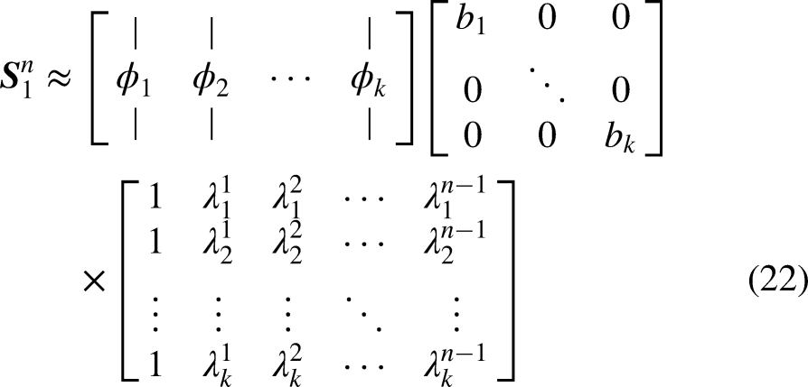
The oscillating frequency and the growth rate of corresponding DMD mode are given by the imaginary part and real part of ${\mathit{\gamma }}_i$ , respectively. Furthermore, the sign of $Re({\mathit{\gamma }}_i)$ denotes the tendency of the temporal evolution of DMD mode. The flow field at any time instant can be obtained using the DMD eigenvalues as

$${\mathit{S}}_1^n\approx \left[\begin{array}{cccc}|& |& & |\\ {\varphi }_1& {\varphi }_2& \cdots & {\varphi }_k\\ |& |& & |\end{array}\right]\left[\begin{array}{ccc}{b}_1& 0& 0\\ 0& \ddots & 0\\ 0& 0& b_k\end{array}\right]\left[\begin{array}{ccccc}1& {\lambda }_1^1& {\lambda }_1^2& \cdots & {\lambda }_1^{n-1}\\ 1& {\lambda }_2^1& {\lambda }_2^2& \cdots & {\lambda }_2^{n-1}\\ ⋮& ⋮& ⋮& \ddots & ⋮\\ 1& {\lambda }_k^1& {\lambda }_k^2& \cdots & {\lambda }_k^{n-1}\end{array}\right]$$

(22)

where $1\le k\le r$ . As shown on the right hand side of equation (22), the first, second, and third matrices represent the DMD modes, the oscillating amplitudes of each DMD mode with diagonal entries are obtained by solving the best fit solution of $\mathbf{\Phi }\mathit{b}={\mathit{s}}_{\mathbf{1}}$ , and the Vandermonde matrix where each row describes the temporal evolution of each DMD mode, respectively.

Computation setup

In the present work, the IBVM flow solver and DMD scheme are employed to capture the dynamic characteristics of stall of flow over a symmetric airfoil. For the computational setup of the IBVM flow solver, the viscous flow past the symmetric airfoil NACA 0012 at the Reynolds number of Re = 1000 is investigated. Due to the advantage of the vortex particle method, the blockage effect, found in Duong et al., ⁴⁷ is neglected due to the satisfaction of farfield boundary condition with the representation of vortex particles. The Reynolds number, non-dimensional time, lift coefficient, and normalized vorticity are defined as

$$Re=\frac{D{U}_{\mathrm{\infty }}}{\nu },t^{*}=\frac{U_{\mathrm{\infty }}t}{D},C_L=\frac{F_y}{\frac{1}{2}{U}_{\mathrm{\infty }}^{2}D}\mathrm{and}{\omega }^{*}=\frac{\mathrm{D}\omega }{{\mathrm{U}}_{\mathrm{\infty }}}$$

(23)

where $t^{*}$ , $D$ and $U_{\mathrm{\infty }}$ are characteristic time, length and velocity, respectively. The net force exerted on the body from the fluid (of unit density) in vortex methods is computed as

$$\mathit{F}(F_x,F_y)=-\frac{d\mathit{I}(I_x,I_y)}{dt}$$

(24)

where $\mathit{I}$ is given by

$$\mathit{I}=\frac{1}{\mathcal{N}-1}{\int }_V\mathit{x}\times \mathit{\omega }dS$$

(25)

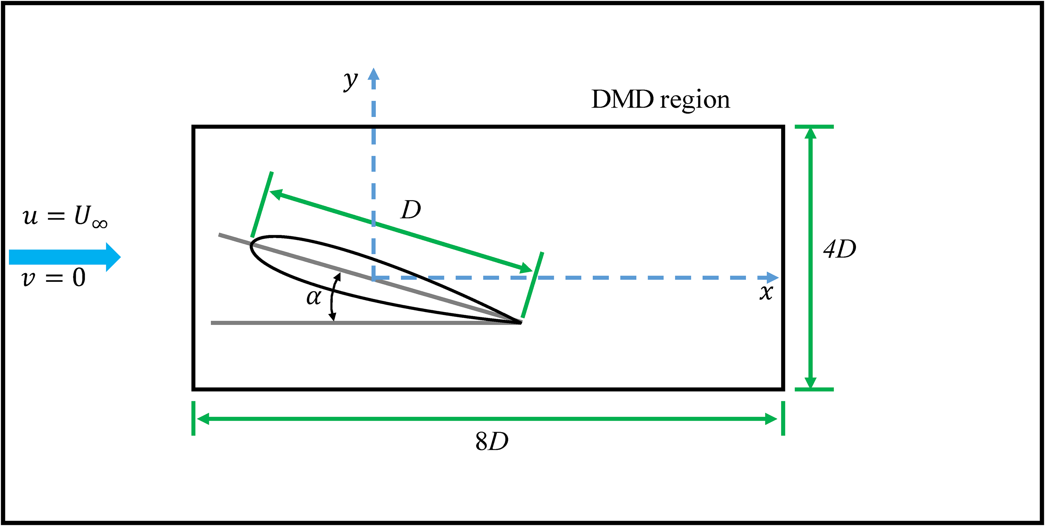
with $\mathcal{N}$ denotes the dimension of the space ( $\mathcal{N}=2$ for a two-dimensional case) and $S$ is the occupied area of the fluid. In vortex element method, $dS$ is equal to particle core size ${\sigma }^2$ . The derivative of the linear impulse (Eq. (25)) is computed using a second-order central difference scheme. To maintain the accuracy of iterative Brinkman penalization, the trailing edge of the airfoil is located between two mesh cells to ensure that the finite thickness is evaluated correctly by penalization. The mollification length ( $2ϵ$ ) is assigned to be $1$ . The time step size is chosen at $△t^{*}={10}^{-3}$ . The tolerance of the residual force was set to $\epsilon ={10}^{-1}$ . To validate the present results with those of the reference work performed by Kurtulus, ⁴¹ the angles of attack $\alpha$ are set as ${20}^{\circ }$ , ${60}^{\circ }$ , and ${90}^{\circ }$ , as shown in Figure 2. The particle core size is defined as $1/275$ at Re =1000, as referred to references.^31,48–50

Figure 2.

Configuration of flow past an airfoil NACA 0012. The confined region ( $8D\times 4D$ ) indicates the region for the analysis of dynamic mode decomposition.

As shown in Figure 3, the vorticity contours of the present results qualitatively agree well with those of reference for three angles of attack. In particular, the sizes of the leading- and trailing-edge vortices of the present work coincide with those of reference. For $\alpha ={60}^{\circ }$ , the Kelvin-Helmholtz vortices that occurred around the trailing edge vortex are also captured by the present result and reference. The comparisons of lift coefficients at three angles of attack are quantitatively performed by Figure 4. As shown in the figure, the lift coefficients of present results collapse those of reference at three angles of attack. The detailed comparison of the lift coefficient of the present results with that of reference is shown in Table 1. The time-mean values, maximum and minimum peaks of $C_L$ , and the Strouhal number at different angles of attack show good agreement (less than $6\text{\%}$ ) with those of the reference. Therefore, the IBVM flow solver has been validated for the case of a separated flow past a symmetric airfoil at high angles of attack at Re =1000.

Figure 3.

Comparision of the vorticity field obtained by IBVM (a) and reference ⁴¹ (b) at $\alpha ={20}^{\circ }$ , $\alpha ={60}^{\circ }$ , and $\alpha ={90}^{\circ }$ .

Figure 4.

Comparision of the vorticity field obtained by IBVM (solid lines) and reference ⁴¹ (red-dashed lines) at $\alpha ={20}^{\circ }$ (a), $\alpha ={60}^{\circ }$ (b), and $\alpha ={90}^{\circ }$ (c).

Table 1.

Comparison of lift coefficient of present results with references at various angles of attack.

AoA		Present	Kurtulus41,51
${20}^0$	${\overline{C}}_L$	0.823 ( $2.5\text{\%}$ )	0.844
	min $C_L$	0.635 ( $3.0\text{\%}$ )	0.616
	max $C_L$	1.169 ( $2.5\text{\%}$ )	1.14
	St	0.553 ( $1.2\text{\%}$ )	0.56
${60}^0$	${\overline{C}}_l$	1.644 ( $5.5\text{\%}$ )	1.734
	min $C_L$	0.973 ( $5.9\text{\%}$ )	1.035
	max $C_L$	2.243 ( $4.5\text{\%}$ )	2.351
	St	0.167 ( $4.3\text{\%}$ )	0.16
${90}^0$	${\overline{C}}_L$	0.079 ( $5.8\text{\%}$ )	0.084
	min $C_L$	$-$ 0.442 ( $3.7\text{\%}$ )	$-$ 0.426
	max $C_L$	0.625 ( $3.8\text{\%}$ )	0.65
	St	0.137 ( $5.4\text{\%}$ )	0.13

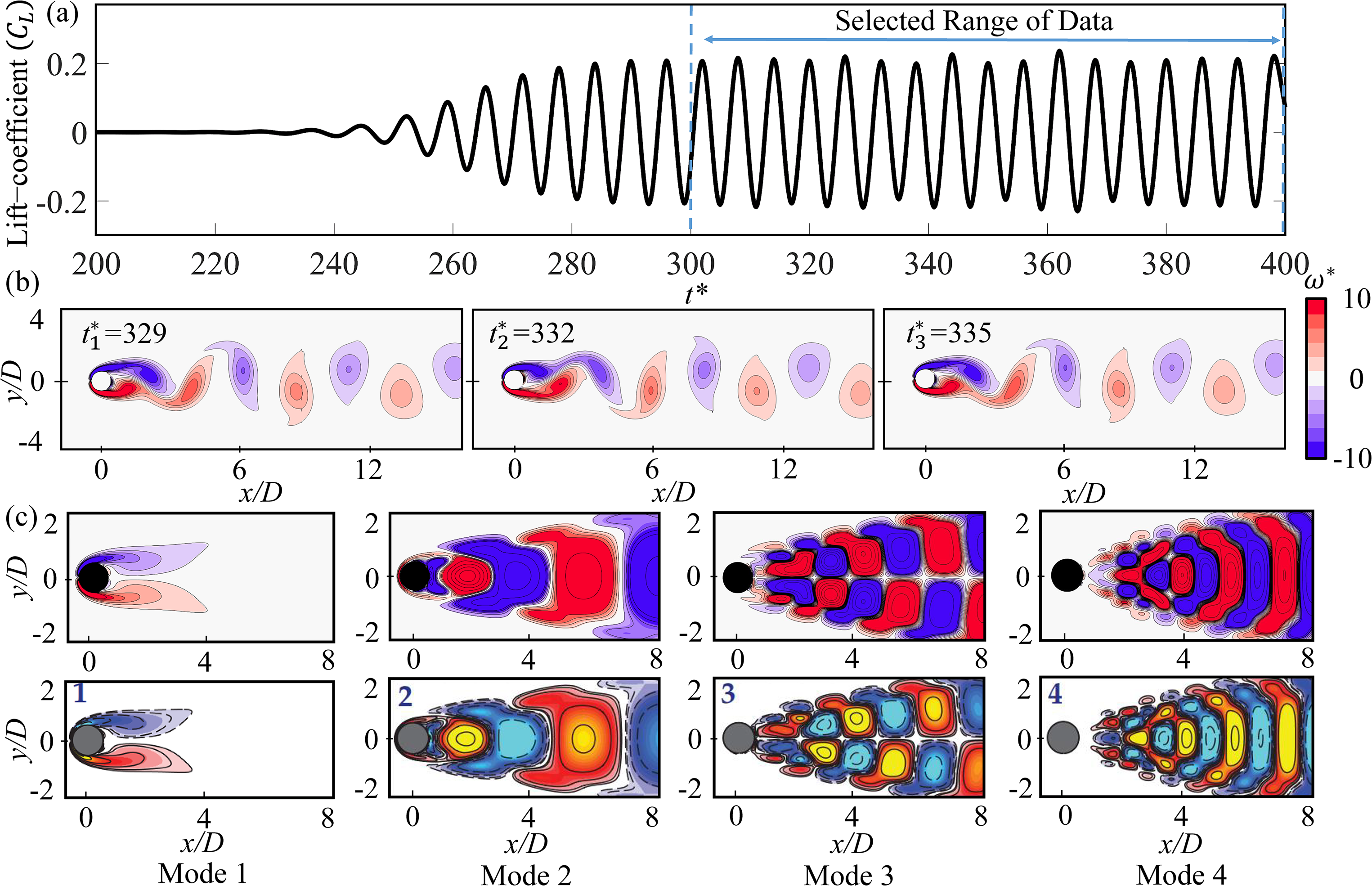
For the computational setup of the DMD scheme, the flow past an impulsively started cylinder at Re =100 is considered. The time step ( $△t^{*}=0.005$ ), the diameter of cylinder $D=1$ , and uniform flow velocity $U_{\mathrm{\infty }}=1$ are considered. The particle core size is set as $1/135$ for Re = 100, as referred to Duong et al. ³¹ All the parameters for iterative Brinkman penalization are set the same as those in the airfoil case. For the IBVM, the data of the entire domain have been used. Since DMD demands high computations and memory resources, to overcome this constraint, DMD is performed in a subdomain ( $8D\times 4D$ ) near the solid body, as shown in Figure 2. The results of DMD depend on the time step between two consecutive snapshots and the total number of snapshots used for the analysis. As shown in Figure 5(a), the range of the snapshot data is selected for 17 vortex shedding cycles, and in each cycle, 50 snapshots are sampled. As shown in Figure 5(c), the first four DMD modes are sampled and compared with those of reference. ⁵² For modes 1, 3, and 4, the top-bottom antisymmetric vorticity contours obtained by present IBVM and DMD agree with those of reference. For mode 2, the top-bottom symmetric contours with spatial harmonic structures about the cylinder centerline of the present work are identical to those of reference. Therefore, the DMD scheme is also validated to show its capability for dynamically modeling the two-dimensional separated flow past a symmetric airfoil. In the next section, the reconstruction of the dynamic stall is performed using the DMD modes obtained from the DMD scheme based on a number of snapshots acquired by the IBVM.

Figure 5.

Dynamic mode decomposition analysis; (a) Time history of lift coefficient; (b) instantaneous vorticity field at three instants (maximum $C_L$ ( $t^{*}=329$ ), zero $C_L$ ( $t^{*}=332$ ), and minimum $C_L$ ( $t^{*}=335$ ); (c) first four DMD modes of vorticity; upper and lower sides show the present results and reference’s results, ⁵² respectively.

Results and discussion

Classification of dominant modes

The wake instability related to the topological vortices is scrutinized by Karasudani and Funakoshi. ⁵³ They found that the opposite sign vortices would alternately roll up, diffuse, and arrange themselves in two parallel straight lines as the vortex spacing ratio exceeds 0.365. The spacing ratio is defined as $h/a$ , where $a$ and $h$ are the longitudinal distance of two vortex centers of the same sign and the transverse distance of two vortex centers of opposite sign, respectively. Before decomposing the dominant frequencies in the wake of the airfoil, the identification of the vortex center is considered following the work of Karasudani and Funakoshi. ⁵³ Accordingly, the vortex center locations ( $x_c,y_c$ ) are computed as

$$x_c=\frac{{\int }_{S}x{\omega }^{*}(x,y)dS}{{\int }_S{\omega }^{*}(x,y)dS},y_c=\frac{{\int }_{S}y{\omega }^{*}(x,y)dS}{{\int }_S{\omega }^{*}(x,y)dS}$$

(26)

Where $S$ is an area at which the vorticity strength $|{\omega }^{*}|$ is greater than the threshold value ( $\beta {\omega }_{max}^{*}$ , where ${\omega }_{max}^{*}$ is maximum value of $|{\omega }^{*}|$ in the vortex region ( $S$ ) and $\beta$ varies in the range of $\beta =0.2-0.4$ ). The larger values of $\beta$ determine the smaller sizes of the vortex. Therefore, $\beta =0.2$ is chosen in this paper for better vortex center computation. Based on the computed vortex center locations, $a$ and $h$ are calculated. Figure 6(a) shows the variations of the vortex spacing ratios $h/a$ at three angles of attack ( $\alpha ={20}^{\circ },{60}^{\circ }$ , and ${90}^{\circ }$ ), the horizontal dashed line represents the vortex spacing ratio of 0.365; Figure 6(b) stands for associated wake structures, where the vertical dashed line represents the approximate boundaries where $h/a=0.365$ . As shown in the figure, these boundaries separate two regimes of vortex frequencies (based on the distance between two opposite sign vortices), signifying the primary mode (left side of the boundary) and the secondary mode (right side of the boundary). The visible spatial distributions of vortices of primary mode (the near wake oscillation) are observed with a time interval two-to-four times the secondary mode (intermediate wake oscillation). Therefore, at least four dominant frequencies are available in the wake of the airfoil over different spatial ranges. Hence, for DMD analysis the dominant modes of the dynamic stall of the airfoil are generally decomposed into mode 1 ( $f_1$ ) for primary mode and mode 2 ( $f_2=2f_1$ ), 3 ( $f_3=3f_1$ ), and 4 ( $f_4=4f_1$ ) for secondary mode, being the harmonics of $f_1$ . Based on the time history of lift coefficients in Figure 4, the frequencies of primary modes at $\alpha ={20}^{\circ },{60}^{\circ }$ , and ${90}^{\circ }$ are calculated as 0.553, 0.167, and 0.14, respectively. The DMD analysis was done by using total of 10 shedding cycles; and in each cycle, 52 snapshots are sampled to extract the reconstructions of the dynamic stall at three angles of attack, the so-called approximations to the Koopman modes. ⁵⁴ Furthermore, since the DMD analysis is based on the normalized vorticity field ( ${\omega }^{*}$ ) extracted from the IBVM, the field of ${\omega }^{*}$ is utilized in the present study for visualization.

Figure 6.

(a) Variations of the vortex spacing ratios $h/a$ at case $\alpha ={20}^{\circ }$ , $\alpha ={60}^{\circ }$ and $\alpha ={90}^{\circ }$ , the horizontal dashed line represents the vortex spacing ratio of 0.365; (b) The associated wake structures, the vertical dashed line represents the approximate boundaries where $h/a=0.365$ .

Figure 7 shows the spatial distribution of the normalized vorticity of the mean mode (the most dominant DMD mode) at three angles of attack. As shown in the figure, at $\alpha ={20}^{\circ }$ , two meandering vorticity structures of opposite signs are observed behind the airfoil, representing the Karman vortex street. Meanwhile, at $\alpha ={60}^{\circ }$ and $\alpha ={90}^{\circ }$ these structures divert and arrange themselves into two separated top-bottom layers near the rear surface of the airfoil and finally converge at some distance downstream.

Figure 7.

(a) Spatial distribution of normalized vorticity of the mean mode at $\alpha ={20}^{\circ }$ , (b) $\alpha ={60}^{\circ }$ and (c) $\alpha ={90}^{\circ }$ .

As shown in Figures 8, 9, and 10, information of all retrieved modes corresponding to $\alpha ={20}^{\circ },{60}^{\circ }$ , and ${90}^{\circ }$ is shown, including the relative position of the corresponding eigenvalues in the unit circle, intrinsic frequency, rate of growth, and amplitude; while for each DMD mode, the spatial distribution of normalized vorticity, the corresponding temporal evolution, and power spectral density are shown. The selected modes, $f_0,f_1$ , $f_2$ , $f_3$ and $f_4$ (denoted as modes 0, 1, 2, 3, and 4, respectively) are highlighted by the red lines, where $f_0$ is the mean mode with zero frequency.

Figure 8.

DMD analysis at $\alpha ={20}^{\circ }$ ; (a) the unit circle; (b) Corresponding growth rate; and (c) mode amplitude by frequency, the red lines represent the chosen modes. From (d) to (g): the spatial distribution of normalized vorticity, temporal evolution $D(t^{*})$ , and power spectral density (PSD) of mode 1 ( $f_1$ ), mode 2 ( $f_2$ ), mode 3 ( $f_3$ ) and mode 4 ( $f_4$ ), respectively.

Figure 9.

DMD analysis at $\alpha ={60}^{\circ }$ ; (a) the unit circle; (b) Corresponding growth rate; and (c) mode amplitude by frequency, the red lines represent the chosen modes. From (d) to (g): the spatial distribution of normalized vorticity, temporal evolution $D(t^{*})$ , and power spectral density (PSD) of mode 1 ( $f_1$ ), mode 2 ( $f_2$ ), mode 3 ( $f_3$ ) and mode 4 ( $f_4$ ), respectively.

Figure 10.

DMD analysis at $\alpha ={90}^{\circ }$ ; (a) the unit circle; (b) Corresponding growth rate; and (c) mode amplitude by frequency, the red lines represent the chosen modes. From (d) to (g): the spatial distribution of normalized vorticity, temporal evolution $D(t^{*})$ , and power spectral density (PSD) of mode 1 ( $f_1$ ), mode 2 ( $f_2$ ), mode 3 ( $f_3$ ) and mode 4 ( $f_4$ ), respectively.

For $\alpha ={20}^{\circ }$ , the mode 1 is retrieved and characterized by frequency $f_1=0.553$ , matching the vortex shedding frequency at $\alpha ={20}^{\circ }$ as computed above. Three harmonic modes of mode 1 are also retrieved, including modes 2, 3, and 4 corresponding to $f_2=1.075$ , $f_3=1.6$ and $f_4=2.15$ . Disregarding the mean mode, the amplitude of mode 1 is shown to be the highest among its harmonics; while the amplitudes of those harmonic modes of mode 1 appear to be relatively small, as shown in Figure 8(c). Figure 8(d) to (g) present the spatial distribution of normalized vorticity, temporal evolution of $D(t^{*})$ , and power spectral density (PSD) of four DMD modes. As shown in the spatial contour of normalized vorticity, the spatial harmonic structures of modes 1, 3, and 4 are shown in the wake of the airfoil. The size of these structures of mode 1 is maximum; while that of mode 3 is larger than that of mode 4. For mode 4, the harmonic structures are dissipated from $x/D=3.8$ to downstream. For mode 2, the spatial harmonic structures are shown from $x/D=0.1$ to $x/D=3.1$ ; while the top-bottom symmetric structures are shown from $x/D=3.2$ to downstream, signifying the Karman vortex shedding street. As shown in the temporal evolution of $D(t^{*})$ and PSD, the amplitudes of modes 1 to 4 are gradually decreasing; while the frequencies of those are gradually increasing.

For $\alpha ={60}^{\circ }$ , the mode 1 is retrieved and characterized by frequency $f_1=0.16$ , matching the vortex shedding frequency at $\alpha ={60}^{\circ }$ as computed above. Three harmonic modes of mode 1 are also retrieved, including mode 2, 3, and 4 corresponding to $f_2=0.32$ , $f_3=0.49$ and $f_4=0.64$ . Disregarding the mean mode, the amplitude of mode 1 is shown to be the highest among its harmonics; while the amplitudes of those harmonic modes of mode 1 appear to be relatively small, as shown in Figure 9(c). Figure 9(d) to (g) present the spatial distribution of normalized vorticity, the temporal evolution of $D(t^{*})$ , and the power spectral density (PSD) of four DMD modes. As shown in the spatial contour of normalized vorticity, the spatial harmonic structures of four DMD modes do not occur in the wake of the airfoil; meanwhile, top-bottom symmetric structures occur at four modes and their phases are shifted between the top and bottom layers. In modes 2, 3, and 4, some noise is also observed near the leading and trailing edge regions due to the flapping of the shear layers. The size of these structures of mode 1 is maximum; while that of modes 2, 3, and 4 is gradually reducing. For four DMD modes, the harmonic structures are dissipated downstream. As shown in the temporal evolution of $D(t^{*})$ and PSD, the amplitudes of modes 1 to 4 are gradually decreasing; while the frequencies of those are gradually increasing, which are identical to what was observed at $\alpha ={20}^{\circ }$ .

For $\alpha ={90}^{\circ }$ , the mode 1 is retrieved and characterized by frequency $f_1=0.15$ , matching the vortex shedding frequency at $\alpha ={90}^{\circ }$ as computed above. Three harmonic modes of mode 1 are also retrieved, including mode 2, 3, and 4 corresponding to $f_2=0.3$ , $f_3=0.44$ and $f_4=0.6$ . Disregarding the mean mode, the amplitude of mode 1 is shown to be the highest among its harmonics; while the amplitudes of those harmonic modes of mode 1 appear to be relatively small, as shown in Figure 10(c). Figure 10(d) to (g) present the spatial distribution of normalized vorticity, the temporal evolution of $D(t^{*})$ , and the power spectral density (PSD) of four DMD modes. As shown in the spatial contour of normalized vorticity, the spatial harmonic structures of four DMD modes do not occur in the wake of the airfoil; meanwhile, top-bottom symmetric structures are observed in modes 1, 2, and 3. In mode 4, the phase is shifted between the top and bottom layers. In modes 2, 3, and 4, some noise is also observed near the leading and trailing edge regions due to the flapping of the shear layers. The size of these structures of mode 1 is maximum; while that of modes 2, 3, and 4 is gradually reducing. For four DMD modes, the dissipation of harmonic structures is not observed, signifying the strong vortex shedding region. As shown in the temporal evolution of $D(t^{*})$ and PSD, the amplitudes of modes 1 to 4 are gradually decreasing; while the frequencies of those are gradually increasing, which are identical to what was observed at $\alpha ={20}^{\circ }$ .

Flow field reconstruction

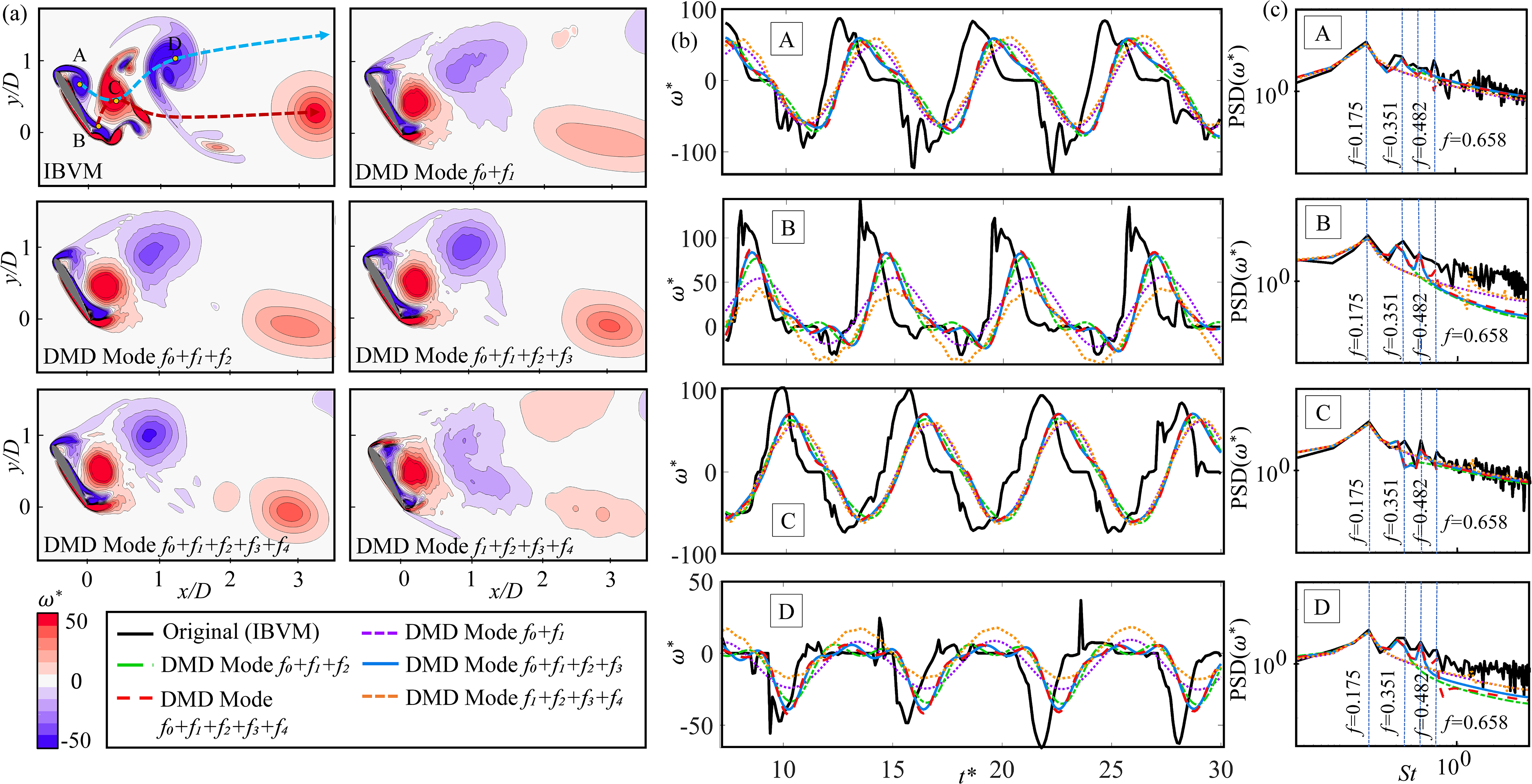
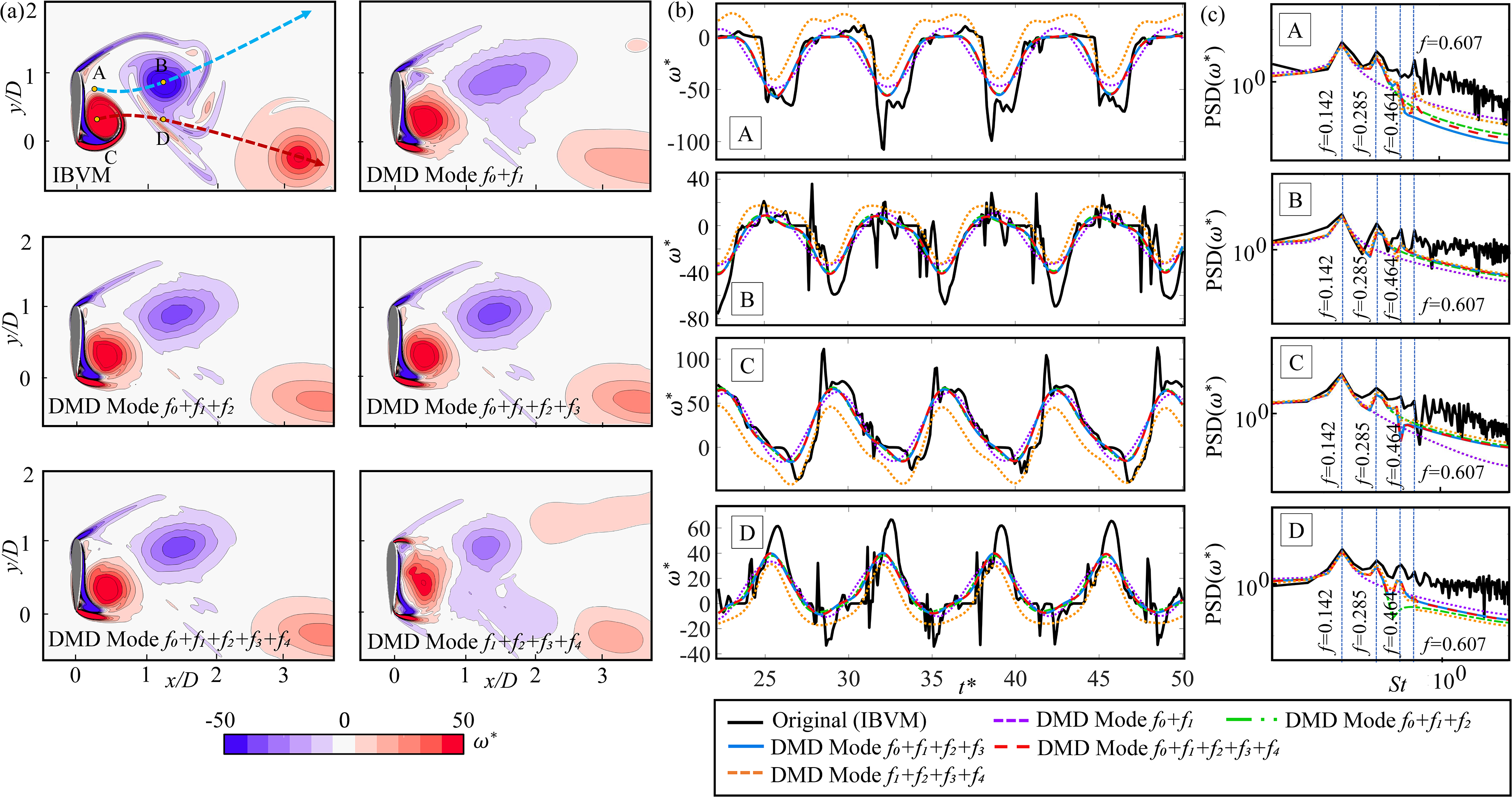
In this section, the DMD analysis is necessitated because of the different dominant frequencies involved within the different spatial ranges of the near and intermediate wake of the airfoil. Since the focus of the present work is the reconstruction of a dynamic stall in the airfoil wake, modes 1, 2, 3, and 4 were extracted with their different combinations for the reconstruction to reveal the role of each mode. Figures 11, 12, and 13 show four combinations of DMD modes performed with zero-frequency mode (mean mode $f_0$ ) corresponding to the time mean vorticity field together with primary mode ( $f_0+f_1$ ), the mean mode together with primary mode and its partial harmonics ( $f_0+f_1+f_2$ , $f_0+f_1+f_2+f_3$ , and $f_0+f_1+f_2+f_3+f_4$ ), and primary mode and its harmonics ( $f_1+f_2+f_3+f_4$ ) at $\alpha ={20}^{\circ }$ , $\alpha ={60}^{\circ }$ , and $\alpha ={90}^{\circ }$ , respectively. In addition, the time histories of normalized vorticity and power spectral densities at different samples located downstream are also extracted for each combination for comparison with those obtained by the IBVM. The blue- and red-dashed arrows stand for the trackings of the clockwise and counterclockwise vortices, respectively. The sample points are planned to be located on these trackings.

Figure 11.

(a) The normalized vorticity contour at $\alpha =20$ , $Re=1000$ at non dimensional time $t^{*}=27.96$ achieved by IBVM and low order reconstructions using combinations of DMD modes; (b) Temporal evolution of local vorticity at reference points; and (c) Power spectral density.

Figure 12.

(a) The normalized vorticity contour at $\alpha =60$ , $Re=1000$ at non dimensional time $t^{*}=9.2$ achieved by IBVM and low order reconstructions using combinations of DMD modes; (b) Temporal evolution of local vorticity at reference points; and (c) Power spectral density.

Figure 13.

(a) The normalized vorticity contour at $\alpha =90$ , $Re=1000$ at non dimensional time $t^{*}=29.7$ achieved by IBVM and low order reconstructions using combinations of DMD modes; (b) Temporal evolution of local vorticity at reference points; and (c) Power spectral density.

As shown in normalized vorticity at $\alpha ={20}^{\circ }$ , $\alpha ={60}^{\circ }$ , and $\alpha ={90}^{\circ }$ , it can be observed that most of the detail of the flow, including the leading and trailing edge vortices, can be reconstructed by using $f_0+f_1$ . By using $f_0+f_1+f_2$ , $f_0+f_1+f_2+f_3$ , and $f_0+f_1+f_2+f_3+f_4$ , the reconstruction becomes more fidelity in terms of the shape of the vortices and the magnitude at the core of the vortices although the small amounts of noises on the rear of the trailing edge occur. Specifically, the combination of $f_0+f_1+f_2+f_3+f_4$ produces the visually identical vorticity field to that of IBVM. It is also presented at the combination of $f_1+f_2+f_3+f_4$ without the inclusion of the mean mode, showing the weak reconstruction of leading and trailing edge vortices and the shear layer at $\alpha ={20}^{\circ }$ ; while those are well reconstructed at $\alpha ={60}^{\circ }$ and $\alpha ={90}^{\circ }$ . In addition, for the reconstruction of intermediate wake, the wake vortices are weakly reconstructed with deformed vortex sizes and deviated locations of vortex center at three angles of attack. Hence, for the near wake, the mean mode plays a crucial role at $\alpha ={20}^{\circ }$ and a minor role at $\alpha ={60}^{\circ }$ and $\alpha ={90}^{\circ }$ ; while for the intermediate wake, the mean mode shows a significant role at three angles of attack. The Kelvin-Helmholtz vortices of small size on the shear layer of the trailing edge (at $\alpha ={60}^{\circ }$ ) and the leading edge (at $\alpha ={90}^{\circ }$ ) obtained from IBVM are not duplicated by all the current DMD mode combinations.

As shown in the temporal evolution of local vorticity at $\alpha =20$ , the result using the combination of $f_1+f_2+f_3+f_4$ is overestimated with that of IBVM at sample point A; while it is underestimated with that of IBVM at sample point B. That is because of the flapping of the shear layer of the leading and trailing edges. The results using combinations of $f_0+f_1+f_2$ and $f_0+f_1+f_2+f_3$ show comparable collapses with those of IBVM at C, D, and E; while the result duplicated by the combination of $f_0+f_1+f_2+f_3+f_4$ collapses very well with those of IBVM at five sample points. Furthermore, the result using the combination of $f_0+f_1$ could not be duplicated well at the peak of normalized vorticity at five sample points. As shown in power spectral density figures, the PSDs of $f_0+f_1+f_2+f_3+f_4$ and $f_1+f_2+f_3+f_4$ agree very well with those obtained by IBVM for the wavenumber ranging from 0.1 to 100 at five sample points; while those of $f_0+f_1$ , $f_0+f_1+f_2$ , and $f_0+f_1+f_2+f_3$ collapses well with those obtained by IBVM in the wavenumber range from 0.1 to 1 and deviates significantly in the wavenumber range from 1.1 to 100 at five sample points. Hence, it confirms the crucial role of the additions of $f_2$ , $f_3$ , and $f_4$ in the flow field duplication.

As shown in the temporal evolution of local vorticity at $\alpha =60$ , the results using all the combinations presented are underestimated from those obtained from IBVM. In particular, the phases of those duplicated from all DMD mode combinations are shifted from those obtained by IBVM. Specifically, at sample point B, the Kelvin-Helmholtz instability signifies the intermittent jumps with high frequencies on the instantaneous vorticity peaks (on top of vorticity time history). These instabilities are not duplicated by all the present DMD mode decompositions. In addition, the phase shiftings are also observed in the PSD figures at four sample points with the frequency (St) ranging from 0 to 1, confirming that the Kelvin-Helmholtz instability shows its remarkable effect in the flow field duplications using the present DMD mode combinations.

As shown in the temporal evolution of local vorticity at $\alpha =90$ , the result using the combination of $f_1+f_2+f_3+f_4$ is overestimated with that of IBVM at the sample points A and B; while it is underestimated with that of IBVM at the sample point C and D. The results duplicated by the combinations of $f_0+f_1+f_2$ , $f_0+f_1+f_2+f_3$ and $f_0+f_1+f_2+f_3+f_4$ collapses very well with that of IBVM at four sample points. Furthermore, the result using the combination of $f_0+f_1$ weakly duplicates at the four sample points. Specifically, it is identical to the case of $\alpha =60$ , the duplications using all DMD mode combinations are weakly performed in the Kelvin-Helmholtz instability signals, signifying the phase shiftings at B and D observed in PSD figures. As shown in the power spectral density, at four sample points, because of the high angle of attack, the PSDs obtained from DMD mode combinations agree well in the narrow frequency range from 0.1 to 0.5; while they deviate significantly from 0.6 to 100. In addition, the effect of $f_3$ and $f_4$ on visual duplication is not very significant in $\alpha ={60}^{\circ }$ and ${90}^{\circ }$ due to their low amplitudes, as shown in Figures 9(c) and 10(c).

Figure 14 presents the contours of the mean vorticity, retrieved by IBVM and the low-order reconstruction using a set of modes $f_0+f_1+f_2+f_3+f_4$ ; the dashed line represents the location of the reference; and normalized mean vorticity at the reference lines at three angles of attack. As shown in the contours of the mean vorticity at $\alpha =20$ , the results using $f_0+f_1+f_2+f_3+f_4$ collapse well with those using IBVM in near airfoil regions; while in the downstream region, they are in good agreement with those of IBVM. Specifically, at higher angles of attack ( $\alpha =60$ and $\alpha =90$ ), the deviation of the vorticity contour gradually increases downstream. As shown in normalized mean vorticity at the reference lines, the result obtained by $f_1+f_2+f_3+f_4$ is underestimated compared to those obtained by IBVM and other DMD mode combinations; while all the DMD mode combination duplicates well the mean vorticity values, showing the important role of the addition of mean modes in reconstructing the mean vorticity field.

Figure 14.

Left: the contour of the mean vorticity, retrieved by IBVM and the low order reconstruction using set of modes $f_0+f_1+f_2+f_3+f_4$ , the dashed line represents the location of the reference line; Right: normalized mean vorticity at the reference lines at $\alpha ={20}^{\circ }$ (a), $\alpha ={60}^{\circ }$ (b), and $\alpha ={90}^{\circ }$ (c).

Dynamic stall duplication

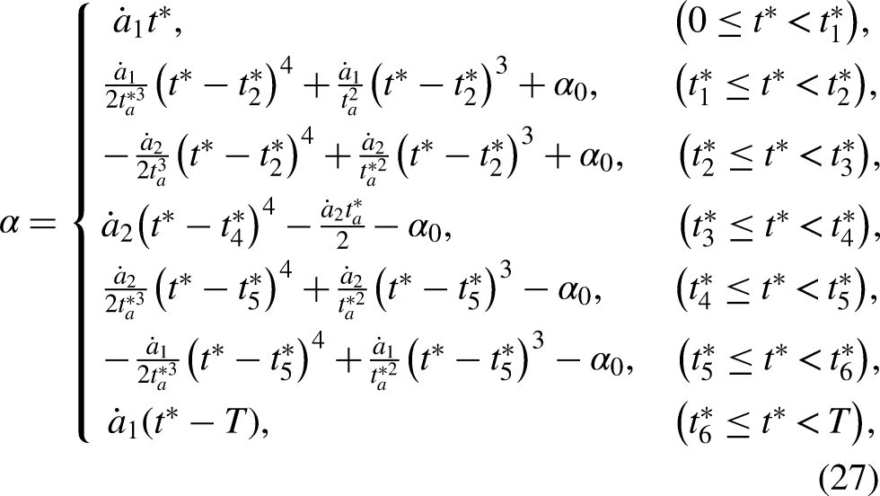
In this section, we investigate the pitching airfoil flow simulation at $Re=U_{\mathrm{\infty }}D/\nu =4000$ with the flow variations ranging from small amplitude ( ${\alpha }_0=4^{\circ }$ ) to large amplitude ( ${\alpha }_0={32}^{\circ }$ ) to predict the forces on an aerofoil in real-time using IBVM and DMD. The airfoil is chosen as a NACA 0018 airfoil for the comparison with experimental results. ⁵⁵ The acceleration time is $t_a^{*}=0.15T$ , where $T=f_p^{-1}$ is the pitching period; and $f_p$ is pitching frequency. The kinematic change is composed of piecewise functions in which the acceleration components are fourth-order polynomials:

$$\alpha =\{\begin{array}{c}{\dot{a}}_1{t}^{*},(0\le t^{*}<t_1^{*}),\\ \frac{{\dot{a}}_1}{2t_a^{*3}}{(t^{*}-t_2^{*})}^4+\frac{{\dot{a}}_1}{t_a^2}{(t^{*}-t_2^{*})}^3+{\alpha }_0,(t_1^{*}\le t^{*}<t_2^{*}),\\ -\frac{{\dot{a}}_2}{2t_a^3}{(t^{*}-t_2^{*})}^4+\frac{{\dot{a}}_2}{t_a^{*2}}{(t^{*}-t_2^{*})}^3+{\alpha }_0,(t_2^{*}\le t^{*}<t_3^{*}),\\ {\dot{a}}_2{(t^{*}-t_4^{*})}^4-\frac{{\dot{a}}_2{t}_a^{*}}{2}-{\alpha }_0,(t_3^{*}\le t^{*}<t_4^{*}),\\ \frac{{\dot{a}}_2}{2t_a^{*3}}{(t^{*}-t_5^{*})}^4+\frac{{\dot{a}}_2}{t_a^{*2}}{(t^{*}-t_5^{*})}^3-{\alpha }_0,(t_4^{*}\le t^{*}<t_5^{*}),\\ -\frac{{\dot{a}}_1}{2t_a^{*3}}{(t^{*}-t_5^{*})}^4+\frac{{\dot{a}}_1}{t_a^{*2}}{(t^{*}-t_5^{*})}^3-{\alpha }_0,(t_5^{*}\le t^{*}<t_6^{*}),\\ {\dot{a}}_1(t^{*}-T),(t_6^{*}\le t^{*}<T),\end{array}$$

(27)

where ${\dot{a}}_1$ and ${\dot{a}}_2$ are pitch rates in regions ( $0\le t^{*}<t_1^{*}$ ) and ( $t_3^{*}\le t^{*}<t_4^{*}$ ), respectively. Both parameters are given by

$$\begin{array}{c}{\dot{a}}_1=\frac{2{\alpha }_0}{\xi T-t_a},\\ {\dot{a}}_2=-\frac{2{\alpha }_0}{(1-\xi )T-t_a}.\end{array}$$

(28)

The asymmetry parameter $\xi$ controls the angle of attack $\alpha$ to peaks of ${\alpha }_0$ at $t_2^{*}=0.5\xi T$ . For the comparison, the reduced frequency $k=\pi f_{p}D/U_{\mathrm{\infty }}=0.22$ , pitching amplitudes of ${\alpha }_0=4^{\circ }$ and ${\alpha }_0={32}^{\circ }$ , and asymmetry parameter $\xi =0.4$ are performed. $t_1^{*}$ , $t_3^{*}$ , $t_4^{*}$ , $t_5^{*}$ , $t_6^{*}$ are respectively evaluated as $t_2^{*}-t_a^{*}$ , $t_2^{*}+t_a^{*}$ , $t_5^{*}-t_a^{*}$ , $T-t_2^{*}$ , $t_5^{*}+t_a^{*}$ . In order to obtain the DMD results, the frame of reference is initially transformed from stationary frame of reference to pitching airfoil frame of reference. Then, the identical procedure is applied to obtain the DMD duplication results on the pitching airfoil frame of reference. Finally, these results are transformed from pitching airfoil frame of reference to stationary frame of reference.

For the DMD analysis, the snapshot number of 200 is taken in 10 pitching periods; and all the results in stationary frame of reference are shown in Figure 15. The mean mode ( $f_0$ ) and four harmonic modes ( $f_1$ , $f_2$ , $f_3$ , and $f_4$ ) are utilized and combined to duplicate the dynamic stall of pitching airfoil. The $f_1$ is equal to pitching frequency ( $f_p$ ) while the harmonics of $f_1$ are equal to $f_2=2f_1$ , $f_3=3f_1$ , and $f_4=4f_1$ . In this figure, the normalized vorticity contours in a pitching period are depicted at pitching amplitudes of ${\alpha }_0=4^{\circ }$ and ${\alpha }_0={32}^{\circ }$ . At ${\alpha }_0=4^{\circ }$ , the DMD results show a good agreement with the IBVM results in the nearfield of $x/D<2.0$ , while the DMD duplications do not capture well the normalized vorticity contour compared to the IBVM results in the farfield of $x/D>2.0$ . At ${\alpha }_0={32}^{\circ }$ , the nearfield and farfield vortices duplicated by DMD generally agree well with those obtained by IBVM except for small noise that occurs near the leading edge of the airfoil. The noise occurence is because of the limited number of snapshots taken in a pitching period for DMD analysis.

Figure 15.

Normalized vorticity contours in a pitching period; (a) the DMD results at ${\alpha }_0=4^{\circ }$ ; (b) the IBVM results at ${\alpha }_0=4^{\circ }$ ; (c) the DMD results at ${\alpha }_0={32}^{\circ }$ ; (d) the IBVM results at ${\alpha }_0={32}^{\circ }$ .

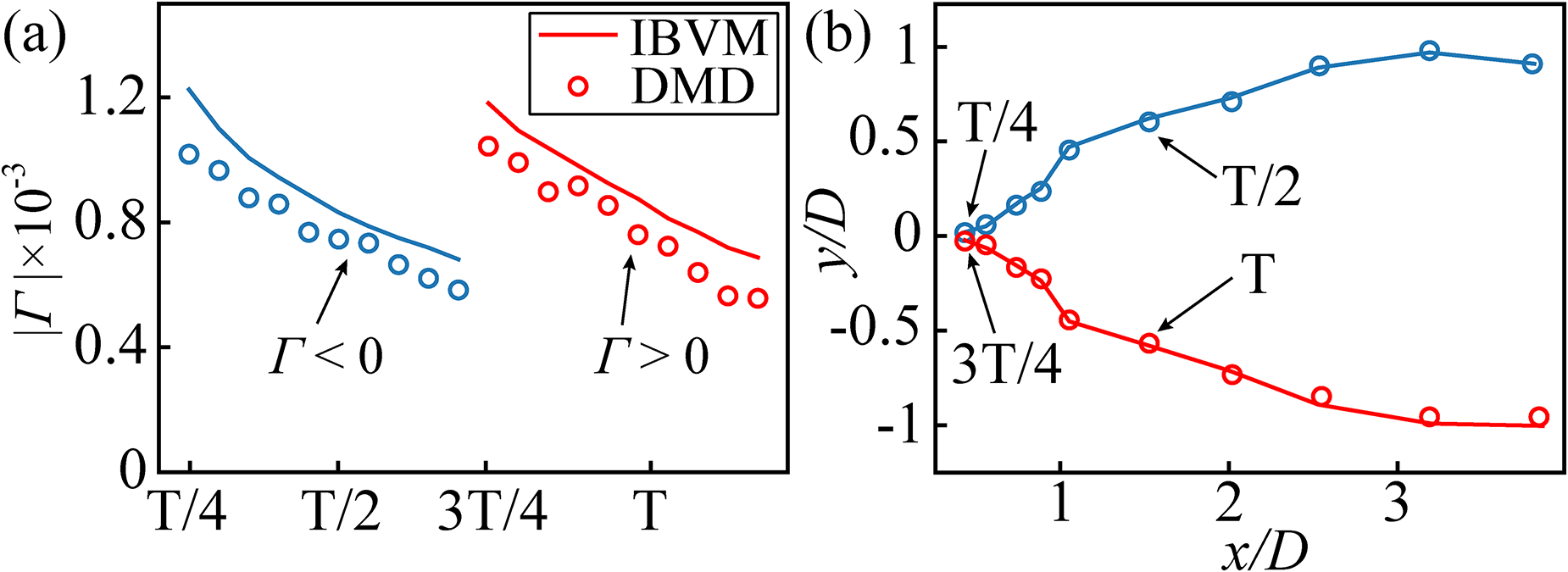
Figure 16 shows the time history of lift coefficient in a pitching period at ${\alpha }_0=4^{\circ }$ and ${\alpha }_0={32}^{\circ }$ . The left vertical axis shows the scale for the lift coefficient while the right vertical axis shows the scale for the pitching kinematic. As shown in the figure, at small ( ${\alpha }_0=4^{\circ }$ ) and large ( ${\alpha }_0={32}^{\circ }$ ) amplitudes the DMD results agree well with the IBVM results. At small amplitude, the phase of experimental result is shifted with that of DMD duplication and IBVM results; while the DMD duplication and IBVM results demonstrate a good agreement with experimental result at large amplitude. Figure 17 shows the evolution of strengths of clockwise (blue) and counterclockwise (red) leading edge vortex in a pitching period and the trackings of the centers of clockwise (blue) and counterclockwise (red) leading edge vortex. These vortices are clearly shown in Figure 15. As shown in Figure 17(a), the magnitudes of vortex stength obtained by DMD duplication are less than those obtained by IBVM. It is reasonable because there are five dominant modes utilized for the DMD analysis. As shown in Figure 17(b), the trackings of the leading edge vortex centers duplicated by DMD modes collapse those obtained by IBVM.

Figure 16.

Time history of lift coefficient in a pitching period at ${\alpha }_0=4^{\circ }$ (a) and ${\alpha }_0={32}^{\circ }$ (b). The left vertical axis shows the scale for lift coefficient while the right vertical axis shows the scale for the pitching kinematic. The present results are compared with experimental result. ⁵⁵

Figure 17.

(a) Evolution of strengths ( $\mathrm{\Gamma }={\omega }^{*}{\sigma }^2$ ) of clockwise (blue) and counterclockwise (red) leading edge vortex in a pitching period; (b) the trackings of the centers of clockwise (blue) and counterclockwise (red) leading edge vortex.

Conclusions

The present paper successfully performed low-order modeling methods, including the iterative Brinkman penalized vortex method and a data-driven dynamic mode decomposition to study the dynamic stall. The data were extracted from the iterative Brinkman penalized vortex method as input for the flow field reconstruction using combinations of the dynamic mode decomposition dominant modes. Several remarks have been pointed out as follows.

In the wake of NACA 0012, there is a boundary separating two regimes of vortex frequencies, signifying the primary mode (left side of the boundary) and the secondary mode (right side of the boundary). The visible spatial distributions of vortices of primary mode (the near wake oscillation) are observed with a time interval two-to-four times the secondary mode (intermediate wake oscillation). Therefore, at least four dominant frequencies are available in the wake of the airfoil over different spatial ranges. Hence, for DMD analysis the dominant modes of the dynamic stall of the airfoil are generally decomposed into mode 1 ( $f_1$ ) for primary mode and mode 2 ( $f_2=2f_1$ ), 3 ( $f_3=3f_1$ ), and 4 ( $f_4=4f_1$ ) for secondary mode, being the harmonics of $f_1$ .

For the most dominant mode (mean mode), at $\alpha ={20}^{\circ }$ , two meandering vorticity structures of opposite signs are observed behind the airfoil, representing the Karman vortex street. Meanwhile, at $\alpha ={60}^{\circ }$ and $\alpha ={90}^{\circ }$ , these structures divert and arrange themselves into two separated top-bottom layers near the rear surface of the airfoil and finally converge at some distance downstream. For flow field reconstruction using DMD dominant modes at three angles of attack, it can be observed that most of the detail of the flow, including the leading and trailing edge vortices, can be reconstructed by using $f_0+f_1$ . By using $f_0+f_1+f_2$ , $f_0+f_1+f_2+f_3$ , and $f_0+f_1+f_2+f_3+f_4$ , the reconstruction becomes more fidelity in terms of the shape of the vortices and the magnitude at the core of the vortices although the small amounts of noises on the rear of the trailing edge occur.

For the duplication of the dynamic stall, at small amplitude of pitching, the DMD results show a good agreement with the IBVM results in the nearfield, while the DMD duplications do not capture well the normalized vorticity contour compared to that of the IBVM in the farfield. At large amplitude of pitching, the nearfield and farfield vortices duplicated by DMD are generally in a good agreement with those obtained by IBVM except for small noise occured near the leading edge of the airfoil. The noise occurence is because of the limited number of snapshots taken in a pitching period for DMD analysis.