Vortex particle method with iterative Brinkman penalization for simulation of flow past sharp-shape bodies

Abstract

This paper presents a Lagrangian vortex method combined with iterative Brinkman penalization for the simulation of incompressible flow past a complex geometry. In the proposed algorithm, particle and penalization domains are separately introduced. The particle domain is for the computation of particle convection and diffusion, while the penalization domain is the enforcement of the wall boundary conditions. In iterative Brinkman penalization, the no-slip boundary condition is enforced by applying penalization force in multiple times within each time step. This enables large time step size reducing computational cost and maintains the capability in handling complex geometries. The method is validated for benchmark problems such as an impulsively started flow past a circular cylinder, normal to a flat plate, and a symmetric airfoil at Reynolds numbers ranging from 550 to 1000. The vorticity and streamline contours, drag, and lift coefficients show a good agreement with those reported in literature.

Introduction

The vortex particle methods early attracted the considerable interest of computational fluid dynamic scientists because of the fact that the advection flows are naturally and precisely simulated with their capability. The vortex particle methods are classified into two branches, including purely Lagrangian (meshless)^1–3 and hybrid vortex methods (remeshed or vortex-in-cell).^4,5 Besides, the combination of vortex element method and enforcement of boundary conditions also plays an crucial role in simulating wall-bounded flows with the presence of complex geometries. There has been many vortex method researches leading to challenging applications in fluid dynamics, such as hydrodynamics, ⁵ flow mediated transport, ⁶ dynamics of rotorcrafts’ turbulent wake, ⁷ vertical axis wind turbines, ⁸ aeroacoustics, ⁹ free jet, ¹⁰ flow controls, ¹¹ and vortex reconnection in viscous fluids. ¹² In the Lagrangian vortex method, the velocity is computed using the unbounded Green’s function, namely Biot-Savart formulation. Since the formulation is direct summation of individual particles within the unbounded domain, the cost is polynomially increased to $N^2$ operations, where $N$ is the particle number. By using the fast multipole method (FMM), the streamfunction, velocity, velocity gradient to evaluate the stretching are obtained with an $N\log N$ computational cost. The vortex diffusion is evaluated by core spreading method ¹³ and particle strength exchange.^14,15 The particle distortion because of Lagrangian effect is dealt with spatial adaption schemes, such as $M_4^{{}^{\prime }}$ interpolation ¹⁴ and splitting and merging.^16–18 In the hybrid vortex method, the Poisson equation is addressed on a Cartesian grid using a fast Poisson solver, which has a computational cost of $M\log M$ , where $M$ is the number of grid nodes. The fast Poisson solver is considered as faster than the fast multipole methods although the free space boundary condition is required. ¹⁹ Specifically, the grid is taken much larger than the vorticity region to ensure the far-field boundary conditions, requiring additional computational memory and cost. ²⁰ In addition, the particle-grid interpolation schemes are employed to deal with the particle distortion issue. The streamfunction is computed by fast-Fourier-transform-based Poisson solver; velocity, diffusion and stretching are computed by centered finite difference on the grid. ²¹ Particles are advected by the newly computed velocity and their circulations are updated after the calculation of vortex diffusion and stretching.

The enforcement of boundary conditions employed in vortex particles methods is divided into meshfree (Nascent vortex element, ³ vortex sheet diffusion ¹⁵ ) and mesh-based immersed boundary method (IBM) approaches. ²¹ It is proved by the fact that the meshfree schemes is difficult to implement and extend to three-dimensional flows around complex geometries, while the mesh-based schemes have shown its capability and simplicity to the complex flow simulations, such as turbulent flows and fluid-structure interaction. In IBM approaches, the Brinkman penalization method, considered as continuous forcing IBM, was popularly utilized by introducing the Brinkman penalization forces into immersed boundary interface to cancel the slip velocity. In the original work, Caltagirone ²² and Angot et al. ²³ introduced a Brinkman penalization method to compute incompressible flows past rigid bodies. The justification of the penalization enforcement was investigated to take into account the fictitious immersed boundaries in an incompressible viscous fluid. In addition, the penalization method was proved to extent straightforwardly to three-dimensional geometries with robust and efficient implementation. Kevlahan and Ghidaglia ²⁴ presented the Brinkman penalization method with efficient pseudo-spectral method on a Cartesian grid for the simulation of two-dimensional flow past obstacles immersed in an incompressible viscous fluid. The enforcement of penalization method is independent with numerical methods and grid used for the computation of diffusion and convection. Mimeau et al. ²⁵ coupled the penalization method with particle-mesh vortex method for simulating flows around complex moving geometries and a porous layer surrounding a rigid body in an incompressible viscous fluid. The penalization technique considerably simplified the vortex method implementation to handle the no-slip boundary condition in the case of complex fluid-structure configurations. Hejlesen et al. ²⁶ further improved the remeshed vortex method with the introduction of iterative Brinkman penalization (IBP) for the enforcement of no-slip boundary condition. The computational cost was remarkably reduced due to the fact that the iterative penalization approach allows larger time steps than what was sufficiently required in Brinkman penalization. In addition, the computed fluid forces acting on the solid boundary using the IBP were in great agreement with those obtained using boundary element method (BEM) and vortex sheet diffusion, which is body-fitted grid approach. It was pointed out that the simplicity and accuracy of the IBP allowed the simple Cartesian grid flexibility up to the simulation of flow around unsteady deforming geometries. Spietz et al. ²⁷ extended the iterative Brinkman penalization method for the simulations of three-dimensional incompressible flows. Although the split-time step approach was utilized in the iterative method to overcome a disadvantage of the iterative schemes, it is not straightforward to extend to 3D flows. In contrast, they pointed out that the conventional non-iterative penalization approach is highly straightforward and expendable to 3D flow simulations. Gillis et al. ²⁸ continued the efficiency improvement of iterative Brinkman penalization approach adopting recycling iterative solver in order to reduce the iteration numbers and therefore greatly decline the computational cost of the penalization steps. The orthonormalized previous solutions were utilized for the recycled subspace.

In the present work, the Lagrangian vortex method and iterative Brinkman penalization are combined for the first time to attain the advantage of the meshfree characteristics and to model complex sharp-shape geometries with high accuracy and convergence. The originality of this work is to extend the flow solver up to the case of simulation of unsteady flows past complex geometries with sharp shape although the present work is capable for the simulation of 3D dynamic flows. The validation for numerical solver, flow simulations and discussions of the results will be given with reference listed in literature. The rest of this paper is organized as follows: section 2 expresses the governing equations and numerical method of Lagrangian vortex method, section 3 describes enforcement of boundary conditions including conventional and iterative Brinkman penalization methods, section 4 gives flow configurations and computational setup, section 5 produces the discussions on results, followed by the conclusions in section 6.

Vortex Particle Method

The Navier-Stokes equations for incompressible flows in primitive variables are written as

$$\mathbf{\nabla }\cdot \mathit{u}=0,\mathit{x}\in \mathrm{\Xi }$$

(1)

$$\frac{\mathrm{\partial }\mathit{u}}{\mathrm{\partial }t}+\mathit{u}\cdot \mathbf{\nabla }\mathit{u}=-\frac{1}{\rho }\mathbf{\nabla }p+\nu {\mathbf{\nabla }}^2\mathit{u},\mathit{x}\in \mathrm{\Xi }$$

(2)

where $\mathrm{\Xi }$ denotes the fluid domain, $\mathit{u}$ is the velocity field, $\rho$ is the fluid density, $\nu$ is the kinematic viscosity while $\mathit{x}$ and $t$ are spatial and time domain, respectively. This system of equations is prescribed by appropriate boundary conditions, which is mentioned in the following section. The Eqs. (1) and (2), expressed in velocity( $\mathit{u}$ )-pressure( $p$ ) form, are transformed into the equivalent velocity( $\mathit{u}$ )-vorticity( $\mathit{\omega }=\mathbf{\nabla }\times \mathit{u}$ ) formulation simply by taking the curl of those as

$$\mathbf{\nabla }\cdot \mathit{\omega }=0,\mathit{x}\in \mathrm{\Xi }$$

(3)

$$\mathbf{\nabla }\times (\frac{\mathrm{\partial }\mathit{u}}{\mathrm{\partial }t}+\mathit{u}\cdot \mathbf{\nabla }\mathit{u})=-\frac{1}{\rho }\mathbf{\nabla }\times \mathbf{\nabla }p+\nu \mathbf{\nabla }\times {\mathbf{\nabla }}^2\mathit{u},\mathit{x}\in \mathrm{\Xi }$$

(4)

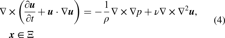
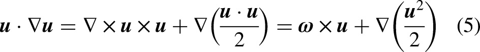
where the pressure term is obviously dropped as $p$ is scalar. By employing the vector identity, the convective term of Eq. (4) is written by

$$\mathit{u}\cdot \mathbf{\nabla }\mathit{u}=\mathbf{\nabla }\times \mathit{u}\times \mathit{u}+\mathbf{\nabla }\left(\frac{\mathit{u}\cdot \mathit{u}}{2}\right)=\mathit{\omega }\times \mathit{u}+\mathbf{\nabla }\left(\frac{{\mathit{u}}^2}{2}\right)$$

(5)

Substituting Eq. (5) into Eq. (4) yields

$$\frac{\mathrm{\partial }(\mathbf{\nabla }\times \mathit{u})}{\mathrm{\partial }t}+(\mathbf{\nabla }\times \mathit{\omega }\times \mathit{u})+\mathbf{\nabla }\times \mathbf{\nabla }\left(\frac{{\mathit{u}}^2}{2}\right)=\nu {\mathbf{\nabla }}^2(\mathbf{\nabla }\times \mathit{u})$$

(6)

The third term of left hand side obviously drops as ${\mathit{u}}^2$ is scalar, and the second term of that is expanded as

$$\mathbf{\nabla }\times \mathit{\omega }\times \mathit{u}=\mathit{u}\cdot \mathbf{\nabla }\mathit{\omega }-\mathit{\omega }\cdot \mathbf{\nabla }\mathit{u}+\mathit{\omega }(\mathbf{\nabla }\cdot \mathit{u})-\mathit{u}(\mathbf{\nabla }\cdot \mathit{\omega })$$

(7)

By enforcing incompressible assumptions (Eqs. (1) and (3)), the last two terms of Eq. (7) are omitted. Hence, by substituting Eq. (7) and imposing the definition of vorticity into Eq. (6), the Navier-Stokes equations in velocity( $\mathit{u}$ )-vorticity( $\mathit{\omega }$ ) formulation are given by

$$\frac{\mathrm{\partial }\mathit{\omega }}{\mathrm{\partial }t}+\mathit{u}\cdot \mathbf{\nabla }\mathit{\omega }=\mathit{\omega }\cdot \mathbf{\nabla }\mathit{u}+\nu {\mathbf{\nabla }}^2\mathit{\omega },\mathit{x}\in \mathrm{\Xi }$$

(8)

The Eq. (8) is expressed in Lagrangian description as

$$\frac{d\mathit{\omega }}{dt}=\mathit{\omega }\cdot \mathbf{\nabla }\mathit{u}+\nu {\mathbf{\nabla }}^2\mathit{\omega },\mathit{x}\in \mathrm{\Xi }$$

(9)

which primarily states that the rate of change of vorticity value from each particle with respect to time is proportional to vortex stretching term and viscous term. To close the problem in Eq. (9), The velocity field is computed by solving the following Poisson equation

$${\mathbf{\nabla }}^2\mathit{u}=\mathbf{\nabla }(\mathbf{\nabla }\cdot \mathit{u})-\mathbf{\nabla }\times (\mathbf{\nabla }\times \mathit{u})$$

(10)

By implying the incompressible flow assumption ( $\mathbf{\nabla }\cdot \mathit{u}=0$ ) and vorticity definition ( $\mathit{\omega }=\mathbf{\nabla }\times \mathit{u}$ ), the following Poisson’s equation relating velocity ( $\mathit{u}$ ) to vorticity ( $\mathit{\omega }$ ) can be obtained.

$${\mathbf{\nabla }}^2\mathit{u}=-\mathbf{\nabla }\times \mathit{\omega }$$

(11)

In order to obtain and update the new position and vorticity of particles, the following equations are computed

$$\frac{d\mathit{u}}{dt}=\mathit{u}(\mathit{x},t)$$

(12)

$$\frac{d\mathit{\omega }}{dt}=\mathit{\omega }\cdot \mathbf{\nabla }\mathit{u}+\nu {\mathbf{\nabla }}^2\mathit{\omega }$$

(13)

Eqs. (12) and (13) are solved using the fourth-order Runge–Kutta method performed by Duong et al. ³ . The stretching term ( $\mathit{\omega }\cdot \mathbf{\nabla }\mathit{u}$ ) is negligible in two-dimensional flow cases, while the diffusion term ( $\nu {\mathbf{\nabla }}^2\mathit{\omega }$ ) is revolved by a particle strength exchange approach, which is further discussed in the following section.

Computation of vortex convection

The Poisson equation (11) recovers the velocity field from vorticity field; and its solution is obtained by an integral representation

$$\mathit{u}=-\frac{1}{2}\int \mathit{K}(\mathit{x}-{\mathit{x}}^{{}^{\prime }})\times \mathit{\omega }\text{d}{\mathit{x}}^{{}^{\prime }}+{\mathit{U}}_0(\mathit{x},t)$$

(14)

where ${\mathit{U}}_0(\mathit{x},t)$ is the solution of the homogeneous solution, and $K(\mathit{x}-{\mathit{x}}^{{}^{\prime }})=(\mathit{x}-{\mathit{x}}^{{}^{\prime }})/|\mathit{x}-{\mathit{x}}^{{}^{\prime }}{|}^d$ denoting the gradient of Green’s function, where $d$ denoting the dimension of the problem. The Eq. (14), called Biot-Savart formulation, is based on the first and second Helmholtz theorems that advect vorticity-carrying particles in inviscid flows, see Cottet and Koumoutsakos ²⁹ . For the velocity computation, the Biot-Savart formulation is discretized as

$${\mathit{u}}_i=\frac{1}{4\pi }\sum _{j=1}^N\frac{{\mathbf{\Gamma }}_j\times ({\mathit{x}}_i-{\mathit{x}}_j)}{{\sigma }^d{|{\mathit{x}}_i-{\mathit{x}}_j|}^d}+{\mathit{U}}_0$$

(15)

where $\mathbf{\Gamma }$ is the strength of particles related to vorticity simply by $\mathbf{\Gamma }={\int }_V\mathit{\omega }\text{d}V$ , $i$ and $j$ presented for the $i^{th}$ and $j^{th}$ particles and $\sigma$ is the particle core size. Although the Biot-Savart law shows the exact satisfaction of far-field boundary condition, the disadvantageous of this method evidently lies on the $O(N^2)$ computational cost due to direct pairwise interactions. In order to reduce the computational cost, the FMM is employed, following the works of Greengard and Rokhlin ³⁰ and Hrycak and Rokhlin ³¹ . The main idea of FMM is to order particles into a tree structure of cubes and exchange particle information among these cube centers using multipole and local expansions. This acceleration technique has reduced the computational cost from $O(N^2)$ to $O(N\log N)$ operations. Figure 1 illustrates the detail of velocity computation with FMM using multipole and local expansions. Basically, the multipole expansion is introduced by group of particles inside the circle of radius $R$ and converged outside the box, while the local expansion is introduced by group of particles outside the circle of radius $R$ and converged within the box.

Figure 1.

Concept of multipole and local expansions in FMM.

Computation of vortex diffusion

For the vortex diffusion computation, taking time derivative of vortex element strength, $\mathbf{\Gamma }={\int }_V\mathit{\omega }\text{d}V$ , leads to

$$\frac{d\mathbf{\Gamma }}{dt}={\int }_V(\frac{\mathrm{\partial }\mathit{\omega }}{\mathrm{\partial }t}+\mathit{u}\cdot \mathbf{\nabla }\mathit{\omega })\text{d}V$$

(16)

Substituting Eq. (9) into Eq. (16), and ignoring the stretching term yield

$$\frac{d\mathbf{\Gamma }}{dt}={\int }_V\left({\mathbf{\nabla }}^2\mathit{\omega }\right)\text{d}V$$

(17)

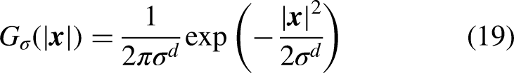
In the present work, viscous term on the right hand side of Eq. (17) is calculated by particle strength exchange (PSE), which approximates the viscous effect by exchanging the strength of surrounding particles. The PSE approach utilized in this paper follows the works of Koumoutsakos and Leonard ³² and Ploumhans and Winckelmans ¹⁴ . The Laplacian operator is approximated by an integral operator and discretized as following

$$\begin{array}{r}{\int }_V\left({\mathbf{\nabla }}^2\mathit{\omega }\right)\text{d}V=2\nu \sum _{j=1}^N\frac{1}{{\sigma }_{ij}^d}{G}_{\sigma }(|{\mathit{x}}_i-{\mathit{x}}_j|)({\sigma }_i^d{\mathbf{\Gamma }}_j-{\sigma }_j^d{\mathbf{\Gamma }}_i)\end{array}$$

(18)

where $G_{\sigma }$ is the Gaussian smoothing kernel expressing particle distribution and defined as

$$G_{\sigma }(|\mathit{x}|)=\frac{1}{2\pi {\sigma }^d}\exp (-\frac{|\mathit{x}{|}^2}{2{\sigma }^d})$$

(19)

The Gaussian smoothing kernel spreads the diffusion effect on a certain particle from surrounding particles with the inversely proportional magnitude to distance. As a particle is closer to another particle, the diffusion effect becomes stronger. ${\sigma }_{ij}^d$ denotes the average core size between a pair of particles interaction. To reduce the computational cost, the PSE only accounts the effect on a particle from other particles, which are located within a supported area at a distance of $5\sigma$ to the corresponding particle position. For the computation stability, the PSE is subjected to a constraint that is given by

$$\frac{\nu \mathrm{\Delta }t}{{\sigma }^d}<\varphi$$

(20)

where $\varphi$ is at value of $\varphi =0.595$ .

Remeshing schemes

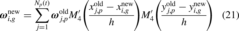
The particle distortion issue arises as the particles move within fluid domain in Lagrangian manner. In order to remedy this situation, the remeshing scheme, introduced by Magni and Cottet ³³ , is applied frequently at every certain time steps to rearrange particles in directly controlled distance between particles, thus securing the solution convergence. It is also obvious that the Lagrangian particles are redistributed on an underlying Cartesian grid, thus renewing the overlapping particle generation. The expression of the remeshing process is here proposed for the two-dimensional case. The three-dimensional case is straightforwardly extended using tensorial product. Let us denote the $p$ and $g$ subscripts as particle and grid, respectively. The ${\mathit{\omega }}_i$ and ${\mathit{\omega }}_j$ subscripts present for new and old vorticities, respectively; $h$ stands for the grid node spacing. The remeshing schemes are conducted as

$${\mathit{\omega }}_{i,g}^{\text{new}}=\sum _{j=1}^{N_p(t)}{\mathit{\omega }}_{j,p}^{\text{old}}{M}_4^{\prime }\left(\frac{x_{j,p}^{\text{old}}-x_{i,g}^{\text{new}}}{h}\right)M_4^{\prime }\left(\frac{y_{j,p}^{\text{old}}-y_{i,g}^{\text{new}}}{h}\right)$$

(21)

and

$${\mathit{\omega }}_{i,p}^{\text{new}}=\sum _{j=1}^{N_g(t)}{\mathit{\omega }}_{j,g}^{\text{old}}{M}_4^{\prime }\left(\frac{x_{j,g}^{\text{old}}-x_{i,p}^{\text{new}}}{h}\right)M_4^{\prime }\left(\frac{y_{j,g}^{\text{old}}-y_{i,p}^{\text{new}}}{h}\right)$$

(22)

for particle-to-grid (P2G) and grid-to-particle (G2P) interpolations, respectively, where $M_4^{\prime }$ is defined as

$$M_4^{\prime }\left(x\right)=\{\begin{array}{cc}1-\frac{5{\left|x\right|}^2}{2}+\frac{3{\left|x\right|}^3}{2},& \text{if}0\le \left|x\right|\le 1\\ \frac{1}{2}{(2-\left|x\right|)}^2(1-\left|x\right|),& \text{if}1\le \left|x\right|\le 2\\ 0,& \text{if}\left|x\right|>2\end{array}$$

(23)

Figure 2 demonstrates the remeshing scheme by a tensorial product employed in this work. The green arrows indicate the 1-D support of the remeshing kernel. The P2G scheme is shown on top sketches; the G2P scheme is shown on bottom sketches. On the top sketches, the empty and filled diamonds stand for before and after kernel support of individual particle; while, on the bottom sketches, the empty and filled circles stand for before and after kernel supports of grid nodes. After P2G remeshing steps, the new overlapping particles are generated. To limit exceeding growth of particles, the limitation of the smallest strength of particle is assigned. In the present work, each new particle, generated with a magnitude of vorticity strength $|\mathbf{\Gamma }|<0.0005|\mathbf{\Gamma }{|}_{max}$ , is removed.

Figure 2.

Illustration of remeshing schemes by a tensorial product. The green arrows indicate the 1-D support of the remeshing kernel. The P2G scheme is shown on top sketches; the G2P scheme is shown on bottom sketches. On the top sketches, the empty and filled diamonds stand for before and after kernel support of individual particle; while, on the bottom sketches, the empty and filled circles stand for before and after kernel supports of grid nodes.

Enforcement of boundary conditions

Conventional Brinkman penalization

Simulation of bounded flows requires an enforcement of appropriate wall boundary conditions in solving the Navier-Stoke equations (Eq. 9). Normally, a boundary condition for solving the vorticity-velocity equations is assigned either as a fixed value (Dirichlet boundary condition) or a derivative value (Neumann boundary condition) to represent for the boundary. In conventional Brinkman penalization IBM, for the boundary representation, the Navier-Stokes vorticity equations, which implicitly include the Brinkman penalization force, are expressed as

$$\frac{d\mathit{\omega }}{dt}=\mathit{\omega }\cdot \mathbf{\nabla }\mathit{u}+\nu {\mathbf{\nabla }}^2\mathit{\omega }+\mathbf{\nabla }\times [\lambda \chi ({\mathit{u}}_s-\mathit{u})]$$

(24)

The penalization method enforces the no-slip boundary condition on the surface of a body in an incompressible flow, by introducing a source term localized around the surface of the body. This source term is added into the momentum equation. The velocity of the flow $\mathit{u}$ is modified by the penalization term as

$$\frac{\mathrm{\partial }\mathit{u}}{\mathrm{\partial }t}=\lambda \chi ({\mathit{u}}_s-\mathit{u})$$

(25)

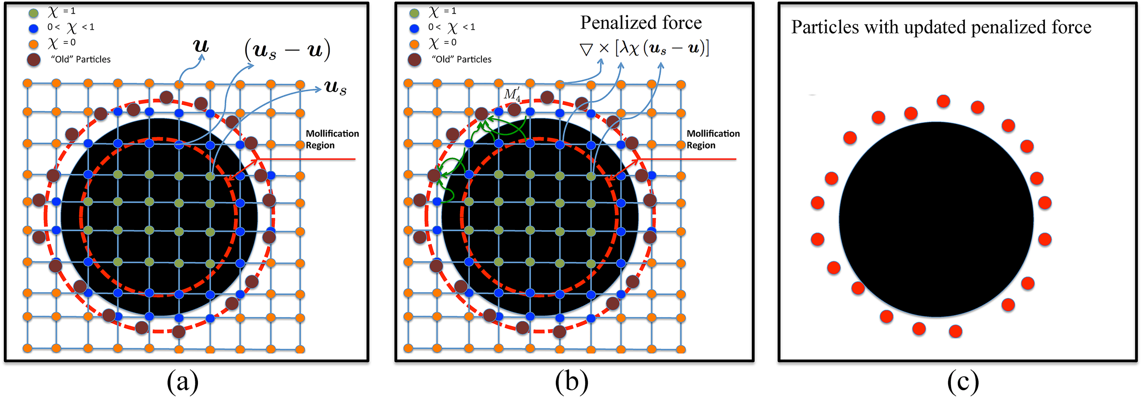
where ${\mathit{u}}_s$ denotes the velocity of the body and $\mathit{u}$ denotes the velocity field of the flow. These variables are enforced to the grid nodes on the interface between the solid boundary and fluid domain (blue-colored nodes in Figure 3). The penalization parameter $\lambda$ has unit $(s^{-1})$ , called reciprocal quantity of the penalization term, and is equivalent to a porosity of the body. The characteristic function $\chi$ is defined by

$$\chi =\{\begin{array}{cc}0,& \text{if}r<-ϵ\\ \frac{1}{2}[1+\frac{r}{ϵ}+\frac{1}{\pi }\sin \left(\pi \frac{r}{ϵ}\right)],& \text{if}\left|r\right|\le ϵ\\ 1,& \text{if}r>ϵ\\ \end{array}$$

(26)

Figure 3.

Schematics of the physical boundary and computational parameterizations of conventional Brinkman penalization method for flow past a solid body.

Hence, the velocity field is corrected with the penalization term which can be evaluated independently. Using an Euler time integration scheme for Eq. (25), the correction can be evaluated implicitly as

$${\mathit{u}}^{n+1}=\frac{{\mathit{u}}^n+\lambda △t\chi {\mathit{u}}_s}{1+\lambda △t\chi }$$

(27)

The penalization term can be expressed in the vorticity formulation as

$$\frac{\mathrm{\partial }\mathit{\omega }}{\mathrm{\partial }t}=\mathbf{▽}\times \left[\lambda \chi ({\mathit{u}}_s-\mathit{u})\right]$$

(28)

This vorticity form of the penalization can be implemented by an explicit evaluation as

$${\mathit{\omega }}^{n+1}={\mathit{\omega }}^n+\mathbf{▽}\times \left[\chi ({\mathit{u}}_s-\mathit{u})\right]$$

(29)

where the penalization parameter $\lambda$ is chosen to be $\lambda =\frac{1}{△t}$ . Hence, the vorticity of flow field ${\mathit{\omega }}^n$ is updated by a correction $\mathbf{▽}\times [\chi ({\mathit{u}}_s-\mathit{u})]$ , which is evaluated by a fourth order central finite differences. At this point, the penalized term $\mathbf{▽}\times [\chi ({\mathit{u}}_s-\mathit{u})]$ is evaluated on the global Cartesian grid nodes (orange, blue and green) as clearly expressed in Figure 3. The Biot-Savart law is employed to calculate the velocity field $\mathit{u}$ ; the velocity of the body ${\mathit{u}}_s$ is an input parameter for the Brinkman penalization. In Figure 3a, the Cartesian grid nodes are regularly generated surrounding boundary with grid spacing $h=△x=△y$ . The grid spacing is set to be equal to the core size of particle $\sigma$ ; the mollification length $2ϵ$ , represented for a porosity of the body (mollification region), is set to be $2\sqrt{2}h$ . At this point, assuming the previously old particles (red nodes) have been remained in the flow field, shown in Figure 3a and b. After this step, the characteristic function $\chi$ is assigned on every grid nodes. Updating the penalization force on blue and green nodes to the old particles in flow field is performed by the G2P interpolation scheme. In this step, the old particles are updated by a vorticity amount from blue and green nodes, showing the new particle generation by Figure 3c. This step closes the enforcement of conventional Brinkman penalization.

Iterative Brinkman penalization

Although the conventional Brinkman penalization method has successfully accommodated the simulation of flow past complex geometries, see Gazzola et al. ³⁴ , it requires a small time step size for the convergence of solution, see Hejlesen et al. ²⁶ . It consequently increases computational cost at significant amount in the case of long time simulations. In addition, the inconsistency of no-though boundary condition was raised due to the local velocity-vorticity relation introduced by conventional penalization. In order to remedy these situations, the iterative Brinkman penalization is proposed within a subset of computational domain. In particular, the particle vorticity is computed from the penalized term and utilized with a constrained numbers of times at each time step to update the particle velocity via elliptical Poisson equation. Hence, the flow consistency is enforced by the iterative process, separating the particle vorticity in the flow field from that introduced by the iterative penalization. In the penalized domain, the computed velocity by the Biot-Savart formulation ( $\overline{\mathit{u}}$ ) is deviated from the imposed velocity in the body ( ${\mathit{u}}_s$ ). Therefore, the iterative penalization method simply alters the second term of the right hand side of the Eq. (29), introducing penalization velocity, ${\mathit{u}}_{\omega }$ , as follows

$$△{\mathit{\omega }}^k=\mathbf{\nabla }\times \left[\chi \left({\mathit{u}}_s-\overline{\mathit{u}}-{\mathit{u}}_{\omega }^{k-1}\right)\right]]$$

(30)

where superscript $k$ indicates the iteration count within each time step. Accordingly, penalization vorticity is updated by

$${\mathit{\omega }}^k={\mathit{\omega }}^{k-1}+△{\mathit{\omega }}^k$$

(31)

The iteration is started by re-computing penalization velocity ${\mathit{u}}_{\omega }^k$ from penalized vorticity ${\mathit{\omega }}^k$ . The evaluation is carried by solving Poisson’s equation relating velocity to vorticity. This equation is solved by the fast Fourier transform (FFT) with free-space boundary condition, indicating that the influence of the solid body at the edge of penalization domain is negligible.

$${\mathbf{\nabla }}^2{\mathit{u}}_{\omega }^k=-\mathbf{\nabla }\times {\mathit{\omega }}^k$$

(32)

A constraint to halt the iteration is defined by the evaluation of penalization force, as suggested by Hejlesen et al. ²⁶ . This constraint is applied as follows

$$△{\mathit{F}}^k=-\rho \frac{1}{△t}\int \mathit{x}\times △{\mathit{\omega }}^k\text{d}V$$

(33)

$${\mathit{F}}^k={\mathit{F}}^{k-1}+△{\mathit{F}}^k$$

(34)

$$\frac{\parallel △{\mathit{F}}^k\parallel }{\parallel {\mathit{F}}^k\parallel }<\epsilon$$

(35)

where $\epsilon$ is a residual force assigned at a small value for a convergence of solution.

Flow configurations and computational setup

As shown by Figure 4a, the comparison of the iterative penalization method with the conventional penalization method is conducted in high-resolution simulations of the early evolution of an impulsively started flow past a circular cylinder at two Reynolds numbers Re = 550. The time step sizes ( $△T=△t{U}_{\mathrm{\infty }}/D$ ) are chosen to be 0.005, where a cylinder of a unit diameter, $D=1$ , is considered with a uniform flow, $U_{\mathrm{\infty }}=1$ . In the following sections, a comparison with the work of Ploumhans and Winckelmans ¹⁴ is presented. The improvement in accuracy over the non-iterative penalization method by presenting the results in term of vorticity contours, streamlines, and drag coefficients, is also demonstrated. Reynolds number, non-dimensional time, and drag coefficients are defined as

$$Re=\frac{D{U}_{\mathrm{\infty }}}{\nu },T=\frac{U_{\mathrm{\infty }}t}{D},\text{and}{C}_D=\frac{F_x}{\frac{1}{2}{U}_{\mathrm{\infty }}D}$$

(36)

Figure 4.

Flow configurations. Left-hand-side figure is the schematic sketch for impulsively started cylinder; Right-hand-side figure is the schematic sketch for impulsively started flat plate.

The net force exerted on the body from the fluid (of unit density) in vortex methods is computed as

$$\mathit{F}(F_x,F_y)=-\frac{d\mathit{I}(I_x,I_y)}{dt}$$

(37)

where $\mathit{I}$ is given by

$$\mathit{I}=\frac{1}{\mathcal{N}-1}{\int }_V\mathit{x}\times \mathit{\omega }dV$$

(38)

with $\mathcal{N}$ denotes the dimension of the space ( $\mathcal{N}=3$ for 3D, $\mathcal{N}=2$ for 2D) and $V$ is the volume occupied by the fluid. For two-dimensional, $V$ is represented as the area occupied by the fluid. In vortex element method, $dV$ is equal to ${\sigma }^d$ . In this case, the particle core sizes are respectively set as $1/135$ and $1/275$ for Re = 550, as referred to Duong et al. ³ . The derivative of the linear impulse (Eq. (38)) is computed using a second-order central difference scheme.

As shown in Figure 4b, a flat plate of a unit length, $L=1$ , is held normal to a unit freestream velocity, $U_{\mathrm{\infty }}=1$ . Reynolds number, non-dimensional time, non-dimensional plate thickness, and the drag coefficient are defined as

$$Re=\frac{L{U}_{\mathrm{\infty }}}{\nu },T=\frac{U_{\mathrm{\infty }}t}{L},H^{*}=\frac{H}{L},\text{and}{C}_D=\frac{F_x}{\frac{1}{2}{U}_{\mathrm{\infty }}L}$$

(39)

where $L$ and $H$ indicate the length and thickness of the flat plate, respectively. The viscous flow normal to a flat plate at a Reynolds number of Re = 1000 is investigated. Due to the enforcement of wall boundary condition with the iterative penalization method, a finite thickness of the plate is required to separate solid and fluid domain in assigning $\chi$ values to apply the Brinkman IBM. In contrast, the finite thickness is not required for boundary element method, see Koumoutsakos and Leonard ³² . To validate our result with that of an infinitely thin flat plate, a convergence study is conducted by varying the plate thickness of $H^{*}=1/50$ , $1/100$ , and $1/200$ , corresponding to a plate thickness of $8$ , $4$ , and $2$ cell lengths, respectively. The edge of the plate is located between two mesh cells to ensure that the finite thickness is evaluated correctly by penalization. The mollification length ( $2ϵ$ ) is assigned to be $0$ and $1$ for the thickness of $H^{*}=1/100$ and $1/200$ , respectively. At thickness of $H^{*}=1/50$ , mollification parameter ( $2ϵ=1$ ) is applied. The time step size is chosen at $△T=△t{U}_{\mathrm{\infty }}/L={10}^{-3}$ . The tolerance of the residual force was set to $\epsilon ={10}^{-1}$ . The particle core size is set as $1/400$ .

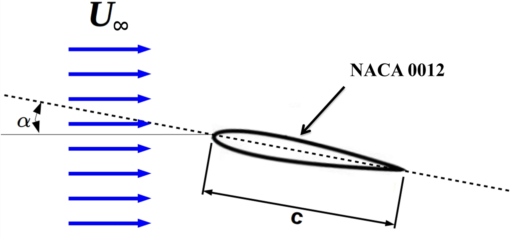
In order to extend the capability of the iterative Brinkman penalization for the flow past the sharp-shape geometry, the comparison of the results of iterative Brinkman penalization with the body-fitted mesh results by Kurtulus ³⁵ is performed for the dynamic stall simulation of the high AoA symmetric airfoil, as shown in Figure 5. The NACA 0012 symmetric airfoil is immersed in the uniform flow at angle of attack (AoA), $\alpha$ . The aerodynamic parameters are specified as follows. The Reynolds number ( $R{e}_c=c{U}_{\mathrm{\infty }}/\nu$ ) based on the airfoil chord length $c$ and the free stream velocity $U_{\mathrm{\infty }}$ is set to be 1000 for most of simulations. The drag coefficient is accordingly computed as $C_D=\frac{F_x}{\frac{1}{2}{U}_{\mathrm{\infty }}c}$ . The AoAs are $5^0,{10}^0,{15}^0$ and ${20}^0$ . The particle core size is defined as $\sigma =0.01$ . The mollification parameter ( $2ϵ=1$ ) is utilized; the tolerance of the residual force was set to $\epsilon ={10}^{-1}$ .

Figure 5.

Configuration of flow past a symmetric airfoil.

Results and discussions

Impulsively started cylinder

The validation and convergence study of iterative and conventional penalization methods are performed in this section. Figure 6 shows contours of vorticity for the impulsively started flow past a circular cylinder at Re= 550 at times $T=t^{*}=t{U}_{\mathrm{\infty }}/D=1,3$ , and 5. Present work is shown on the left hand side column, where the red and black contours represent for the results of the iterative penalization method and the conventional penalization method, respectively. The results obtained using BEM by Ploumhans and Winckelmans ¹⁴ are shown on the right hand side column, where dashed and continuous lines stand for contours of positive and negative vorticity, respectively. There are two vortices formed behind the cylinder, including the primary vorticity in the recirculation zone and the secondary vorticity that remains confined near the cylinder. In general, the present results obtained from conventional and iterative penalization are in a good agreement with BEM. However, the results from the iterative penalization method are compared to those of the conventional penalization method, showing a slight difference at $T=1$ . At $T=3$ and $5$ , the vorticity contour from conventional penalization method expresses larger vortical structures in term of length and height than that obtained by the iterative penalization method.

Figure 6.

Contours of vorticity for the impulsively started flow past a circular cylinder at Re= 550 at times $T=t^{*}=t{U}_{\mathrm{\infty }}/D=1,3$ , and 5. Present work is shown on the left hand side column, where the red and black contours represent for the results of the iterative penalization method and the conventional penalization method, respectively. The results obtained using BEM by Ploumhans and Winckelmans ¹⁴ are shown on the right hand side column, where dashed and continuous lines stand for contours of positive and negative vorticity, respectively.

To further quantify this observation, Figure 7 shows the evolution of the maximum length (left) and the maximum height (right) at recirculation zone for the impulsively started flow past a circular cylinder at Re= 550. The results of the iterative penalization method and the conventional penalization method are shown in red squares and blue triangles, respectively; the results obtained using BEM by Ploumhans and Winckelmans ¹⁴ are shown on the black circles. It is observed that, at each time, the size of recirculation zone by the iterative penalization method is more approaching the reference than that by conventional penalization method.

Figure 7.

The evolution of the maximum length (left) and the maximum height (right) at recirculation zone for the impulsively started flow past a circular cylinder at Re= 550. The results of the iterative penalization method and the conventional penalization method are shown in red squares and blue triangles, respectively; the results obtained using BEM by Ploumhans and Winckelmans ¹⁴ are shown on the black circles.

Figure 8 interprets the comparison of the streamlines for the impulsively started flow past a circular cylinder at Re= 550 obtained by the iterative penalization method (red) and the conventional penalization (black) at times $T=1$ and 3. The results of upstream streamlines collapse very well between conventional penalization method and iterative penalization method, while downstream streamlines show a slight deviation in recirculation zone. It is interesting to observe that, as time evolves, the representation of streamlines surrounding secondary vortex by iterative penalization is better than those resolved from conventional penalization, as clearly seen in Figure 8b. As a result, the viscosity confined to the surface of cylinder is resolved more appropriately with iterative penalization approach.

Figure 8.

Comparison of the streamlines for the impulsively started flow past a circular cylinder at Re= 550 obtained by the iterative penalization method (red) and the conventional penalization (black) at times $T=1$ (a) and 3 (b).

Figure 9a reports the calculated drag coefficients for the impulsively started flow past a circular cylinder at Re= 550; the results of the iterative penalization method and those of conventional penalization method are shown by red and blue lines, respectively. The results obtained using BEM by Ploumhans and Winckelmans ¹⁴ are shown by dashed line; the results obtained using the conventional penalization method with vortex-in-cell method by Rasmussen et al. ²¹ are shown by cross symbols. The continuous gray line show the raw data of non-iterative Brinkman penalization, where the blue line shows its averaged data using six degree polynomial curve fitting method. The calculated drag force coefficients by the iterative penalization method shows a better agreement with the results by Ploumhans and Winckelmans ¹⁴ than that of the conventional penalization method. It is seen that the conventional penalization method produces higher values of drag coefficients than those from iterative penalization and the reference, which is consistent to the previous observation of vorticity contours expressed in Figure 6. In particular, the larger recirculation zone resolved by conventional penalization produces higher drag coefficients than that obtained from iterative penalization.

Figure 9.

(a): the calculated drag coefficients for the impulsively started flow past a circular cylinder; (b): the global residual errors of drag coefficients for the impulsively started flow past a circular cylinder at $T=3$ , 3.5, 4, 4.5, and 5.

Figure 9b reports the computed global residual errors of drag coefficients for the impulsively started flow past a circular cylinder at Re= 550, shown on left hand side at $T=3$ , 3.5, 4, 4.5, and 5. The results of iterative penalization method and the conventional penalization method are shown by red and blue lines, respectively. The global residual errors is computed to investigate the residual velocity inside the penalization domain as following

$$e_{residual}=\frac{1}{U_{\mathrm{\infty }}}\sqrt{\frac{1}{V}{\int }_V\chi \left|\right|{\mathit{u}}_s-\mathit{u}{\left|\right|}^{2}dV}$$

(40)

It is clearly observed that the errors of the iterative penalization method is smaller than that of the conventional penalization method. According to the global residual investigation, it is fair to note that the iterative penalization method produces closer results to the unique solution of BEM by Ploumhans and Winckelmans ¹⁴ than those obtained from the conventional penalization method.

Impulsively started flat plate

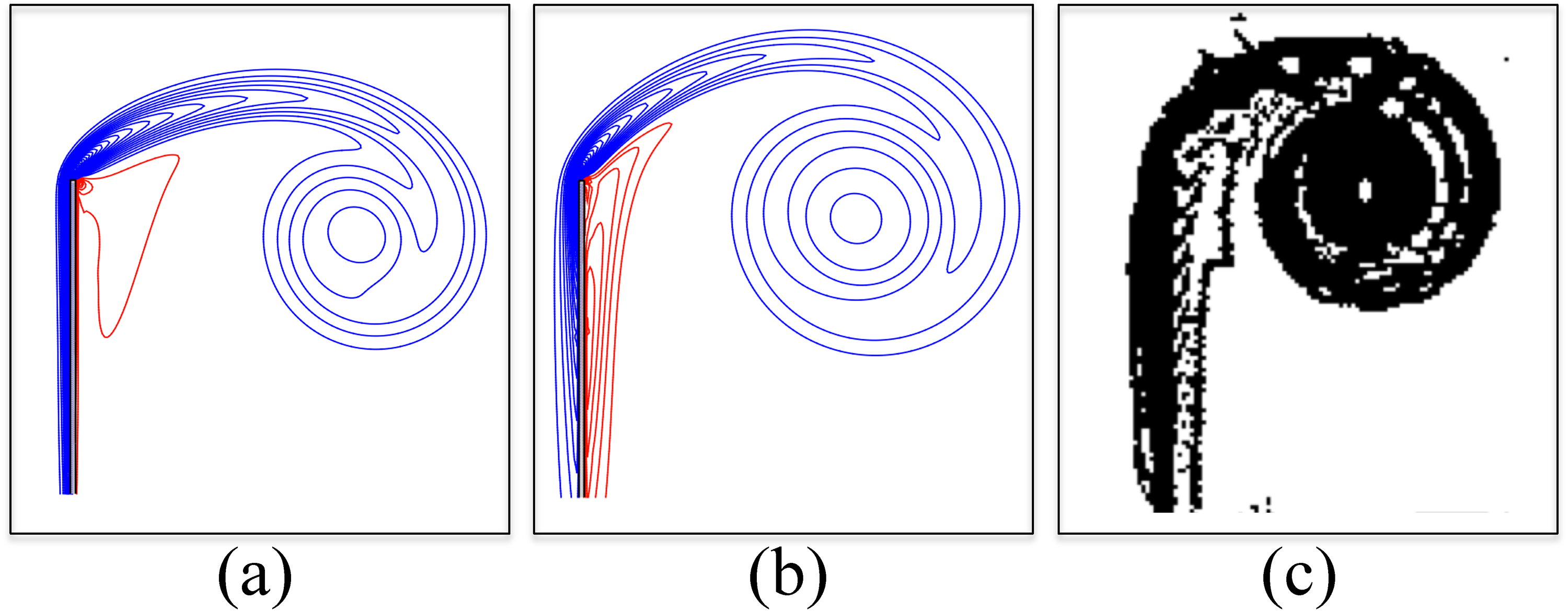
To reveal the advantage of the iterative penalization method on the treatment of complex geometries, the numerical validation in the case of infinitesimally thinned flat plate normal to the flow is investigated in this section. Figure 10 depicts the contours of streamlines for an impulsively started flow normal to uniformly accelerated flat plate at $H^{*}=1/50$ , 1/100, and 1/200 obtained by the conventional penalization method (black) and the iterative penalization method (red) at times $T=0.2$ , 0.5, and 1.0. The streamlines results, obtained by the iterative penalization method, significantly improve the flow field evaluation. Specifically, the streamlines generated by conventional penalization method cross flat plate geometries, thus indicating that the spurious velocity inside the geometry is not cancelled; while the streamlines produced by iterative penalization method detaches the center line of the flat plate, thus forming the stagnation point at frontal surface. It is fair to note that the spurious velocity is eliminated by the iterative penalization method, which is independent with the infinitesimal thickness of the flat plate. From the figure, it is interesting to reveal that due to the elimination of the spurious velocity the recirculation zone behind the rear flat plate surface is physically corrected.

Figure 10.

The contours of streamlines for an impulsively started flow normal to uniformly accelerated flat plate at $H^{*}=1/50$ , 1/100, and 1/200 obtained by the conventional penalization method (black) and the iterative penalization method (red) at times $T=0.2$ (a), 0.5 (b), and 1.0 (c).

Figure 11 shows the contours of vorticity for an impulsively started flow normal to a uniformly accelerated flat plate at $H^{*}=1/200$ and Re =1000 as obtained by the conventional penalization (a), the iterative penalization method (b) with positive values (red) and negative values (blue), and the results from reference ³⁶ (c) at non-dimensional time $T=0.5$ . As the primary vorticity (blue) is forming the recirculation zone, the secondary vortices (red) remain attached to the surface of the flat plate. As shown by Figure 11a and b, the secondary vortices contours (red) generated by the iterative penalization method remain a vorticity layer attached to the rear surface of the flat plate while the contour by the conventional penalization method exist only on the tip of the flat plate, which is non-physical. Furthermore, the primary and secondary vortices produced by iterative penalization method also agree well with the reference.

Figure 11.

The contours of vorticity for an impulsively started flow normal to a uniformly accelerated flat plate at $H^{*}=1/200$ and Re =1000 as obtained by the conventional penalization (a), the iterative penalization method (b) with positive values (red) and negative values (blue), and the results from reference ³⁶ (c) at non-dimensional time $T=0.5$ .

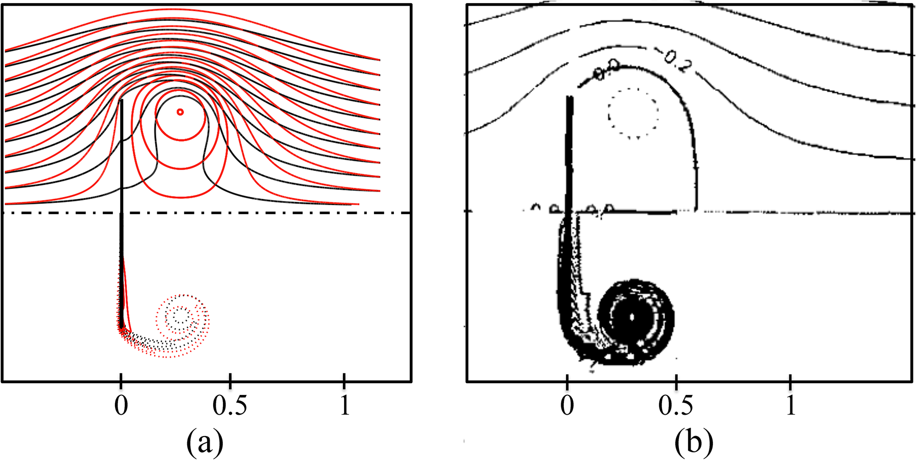
Figure 12 reproduces the contours of streamlines and vorticity for an impulsively started flow normal to a uniformly accelerated flat plate at $H^{*}=1/200$ and Re =1000. Figure 12a shows continuous and dashed lines stands for streamline and vorticity contours, respectively, while the red and black lines stands for the results of the iterative penalization and the conventional penalization, respectively. Figure 12b shows the results from reference ³⁶ at non-dimensional time $T=0.5$ . The streamlines, the primary and secondary vortices produced by iterative penalization method are in a good agreement with those computed by reference.

Figure 12.

The contours of streamlines and vorticity for an impulsively started flow normal to a uniformly accelerated flat plate at $H^{*}=1/200$ and Re =1000. (a): continuous and dashed lines stands for streamline and vorticity contours, respectively, while the red and black lines stands for the results of the iterative penalization and the conventional penalization, respectively; (b): the results from reference ³⁶ at non-dimensional time $T=0.5$ .

Figure 13 depicts the calculated drag coefficients for an impulsively started flow normal to uniformly accelerated flat plate at Re=1000. Continuous and colored-dashed lines respectively represent for the iterative penalization method and the conventional penalization method at $H^{*}=1/50$ (blue), 1/100 (green), and 1/200 (red); Black dashed line show the result obtained using BEM by Koumoutsakos and Shield ³⁶ . The close-up figure is shown on the right hand side. At the early stage of the simulation, the present results deviate from the reference due to the numerical instability; while at latter stage from $T=0.22$ the numerical stability remains. A remarkable difference of drag coefficients is noticed between the conventional and the iterative penalization method. In addition, the drag coefficients produced by iterative penalization method collapse to the reference better than those obtained from conventional penalization method.

Figure 13.

The calculated drag coefficients for an impulsively started flow normal to uniformly accelerated flat plate at Re=1000. Continuous and colored-dashed lines respectively represent for the iterative penalization method and the conventional penalization method at $H^{*}=1/50$ (blue), 1/100 (green), and 1/200 (red); Black dashed line show the result obtained using BEM by Koumoutsakos and Shield. ³⁶

Separated flows around NACA 0012

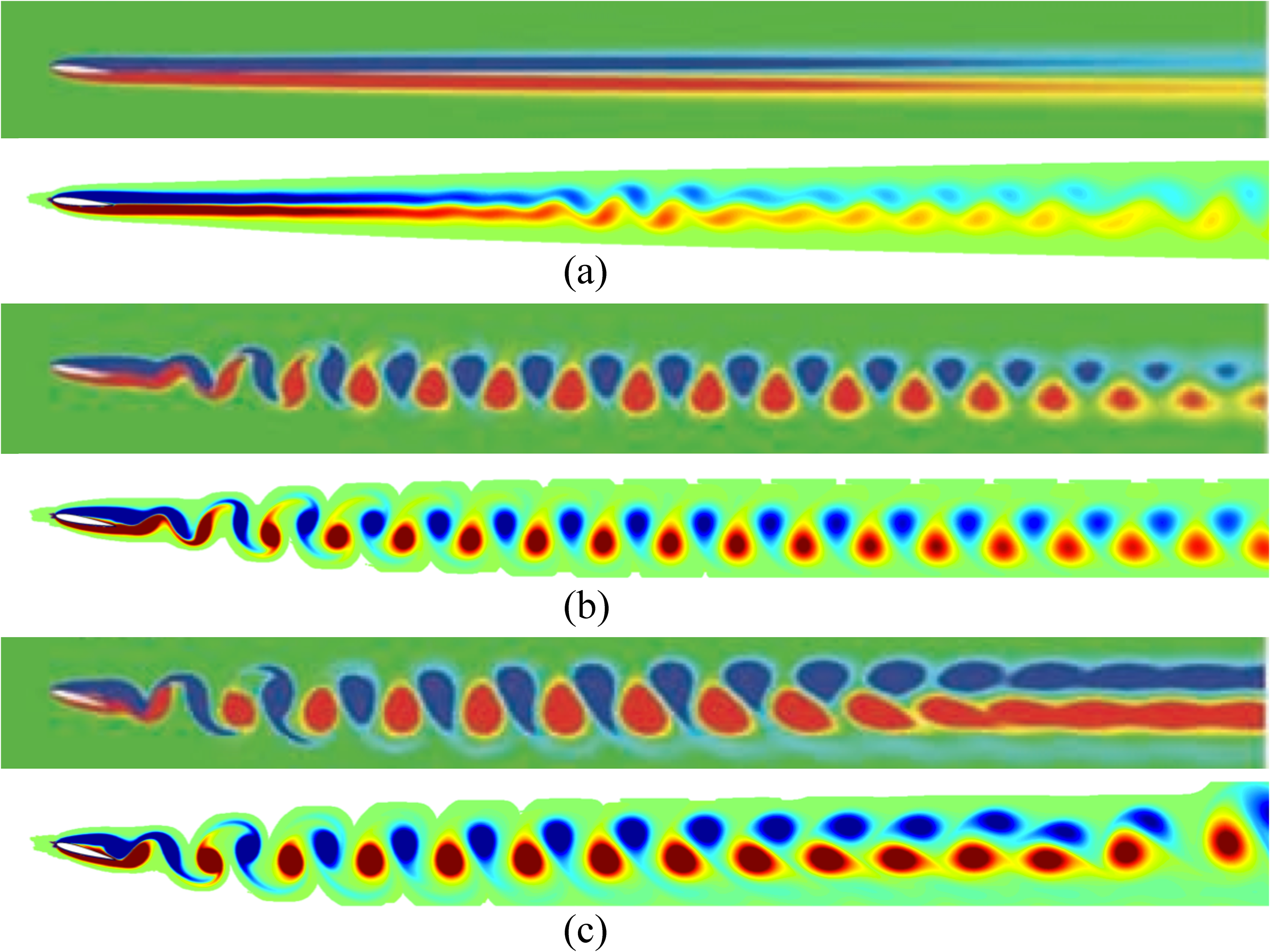
In this section, the simulation of the separated flow over NACA0012 is performed at several angles of attack ranging from $5^0$ to ${20}^0$ to show the capability of iterative Brinkman penalization for the treatment of sharp-shape geometries by comparing the aerodynamic coefficients and vortex shedding mechanism with those listed in literature. Figure 14 produces the comparisons of time history of lift coefficient of present results with those obtained from Kurtulus ³⁵ ; the black continuous and dashed lines represents for present and reference results, respectively; the dotted line stands for the mean value of present lift coefficient. As shown in the figure, there is no separation vortex in the rear of the NACA0012 at the AoA= $5^0$ , thus indicating that flow is steady; and the present result approach well with the reference. At $\mathrm{AoA}={10}^0$ , ${15}^0$ and ${20}^0$ , the trailing-edge vortex (TEV) and leading-edge vortex (LEV) are shedding periodically, showing the oscillations of lift coefficient. The amplitude of the fluctuation of $C_l$ becomes larger as the AoA increases. The present results collapse very well with the reference at the beginning stage of the simulation at all angles of attack. For latter stage, the phases of present results are shifted compared to the reference although the averaged and magnitude values agree very well with those obtained by the reference. The detailed comparison of the lift coefficient of present results with that of reference is shown in Table 1. The time-mean values, maximum and peaks of $C_l$ at different angles of attack show a good agreement with those of the reference.

Figure 14.

Comparisons of time history of lift coefficient of present results with those obtained from Kurtulus ³⁵ ; the black continuous and dashed lines represents for present and reference results, respectively; the dotted line stands for the mean value of present lift coefficient; (a): $\mathrm{AoA}=5^0$ , (b): $\mathrm{AoA}={10}^0$ , (c): $\mathrm{AoA}={15}^0$ , (d): $\mathrm{AoA}={20}^0$ .

Table 1.

Comparison of lift coefficient of present results with references at various angles of attack.

AoA		present	Kurtulus 35
$5^0$	${\overline{C}}_l$	0.233	0.236
	min $C_l$	0.232	0.235
	max $C_l$	0.235	0.237
${10}^0$	${\overline{C}}_l$	0.414	0.413
	min $C_l$	0.376	0.377
	max $C_l$	0.454	0.449
${15}^0$	${\overline{C}}_l$	0.655	0.657
	min $C_l$	0.466	0.468
	max $C_l$	0.887	0.889
${20}^0$	${\overline{C}}_l$	0.843	0.844
	min $C_l$	0.635	0.636
	max $C_l$	1.169	1.17

Figure 15 depicts the comparisons of vorticity contours of the present results with those obtained from Kurtulus ³⁵ at three different AoAs. The figure supports all the differences discussed in the Figure 14, which relate to the appearances of LEV and TEV and also vortexes shed behind the symmetric airfoil. In general, for the shedding of the LEV and TEV, the present results are identical with those computed by reference although there are some differences of vortex shedding distributions in the far wake. However, their influences to the aerodynamic coefficients are minor.

Figure 15.

Comparisons of vorticity contours of the present results with those obtained from Kurtulus ³⁵ at three different AoAs; (a): $\mathrm{AoA}=5^0$ , (b): $\mathrm{AoA}={10}^0$ , (c): $\mathrm{AoA}={15}^0$ .

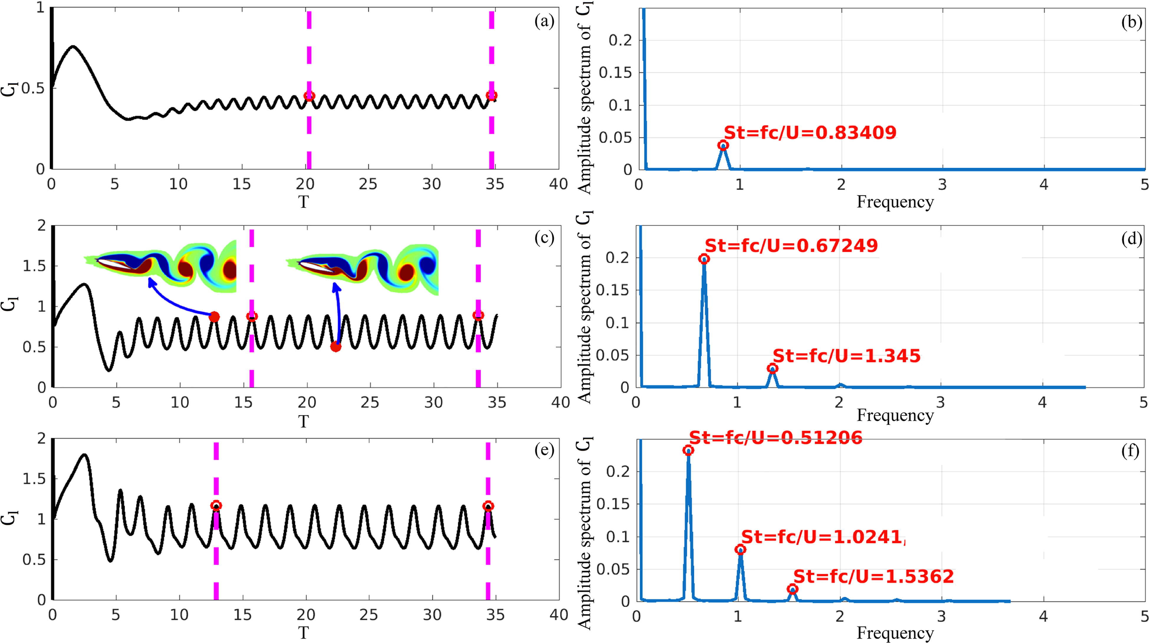
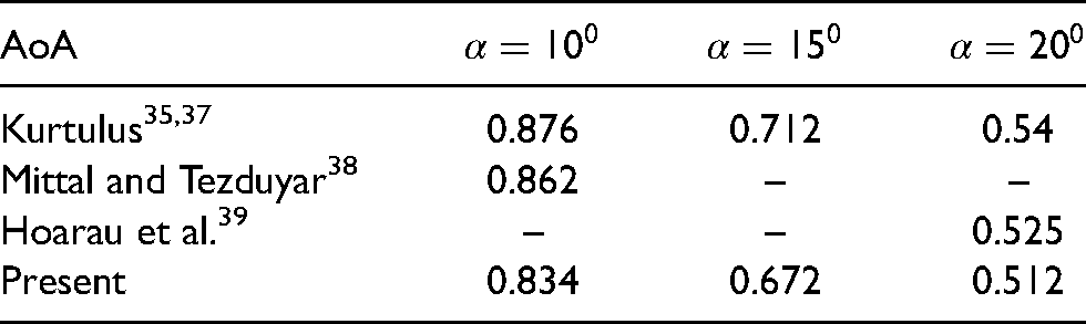
The way to describe the regularity of vortex shedding phenomenon (oscillating flow mechanisms) is the calculation of Strouhal number ( $St$ ). The Strouhal number is defined as $St=\frac{fc}{U_{\mathrm{\infty }}}$ . In Figure 16, left column figures show time history of lift coefficient at three different AoAs (Figure 16a: $\mathrm{AoA}={10}^0$ , Figure 16c: $\mathrm{AoA}={15}^0$ , Figure 16e: $\mathrm{AoA}={20}^0$ ), and instantaneous vorticity contours at some instantaneous times; right column figures show amplitude spectrum of lift coefficient at three different AoAs (Figure 16b: $\mathrm{AoA}={10}^0$ , Figure 16d: $\mathrm{AoA}={15}^0$ , Figure 16f: $\mathrm{AoA}={20}^0$ ). The comparison of Strouhal numbers of the present results with references are summarized in Table 2. In general, the present results agree very well with those listed in literature. In the case of $\mathrm{AoA}={10}^0$ as shown in Figure 16c, when the magnitude of $C_l$ oscillation is maximum, the size of LEV is maximum. Oppositely, when the magnitude of $C_l$ oscillation is minimum, the size of LEV is minimum.

Figure 16.

Left column figures show time history of lift coefficient at three different AoAs ((a): $\mathrm{AoA}={10}^0$ , (c): $\mathrm{AoA}={15}^0$ , (e): $\mathrm{AoA}={20}^0$ ), and instantaneous vorticity contours at some instantaneous times; right column figures show amplitude spectrum of lift coefficient at three different AoAs ((b): $\mathrm{AoA}={10}^0$ , (d): $\mathrm{AoA}={15}^0$ , (f): $\mathrm{AoA}={20}^0$ ). The magenta dashed lines show the time period to take the samples for the calculation of Strouhal numbers.

Table 2.

Comparison of strouhal numbers of present results with those of references at various AoAs.

AoA	$\alpha ={10}^0$	$\alpha ={15}^0$	$\alpha ={20}^0$
Kurtulus35,37	0.876	0.712	0.54
Mittal and Tezduyar 38	0.862	–	–
Hoarau et al. 39	–	–	0.525
Present	0.834	0.672	0.512

Conclusions

The present paper successfully combines the iterative Brinkman penalization with the algorithm of Lagrangian vortex method and demonstrates the capability of the algorithm for the treatment of sharp-shape geometries. The accuracy improvement of the iterative penalization method over the conventional penalization method is also investigated by examining several benchmark tests.

In case of an impulsively started flow past a circular cylinder at Re = 550, the drag coefficients measured by the iterative penalization method is more accurate than that by the conventional penalization method. The size of recirculation zone by the iterative penalization method is more approaching the reference than that by conventional penalization method.

In the case of impulsively started flow normal to a flat plate, the streamlines results, obtained by the iterative penalization method, significantly improve the flowfield evaluation. Specifically, the streamlines generated by conventional penalization method cross flatplate geometries, thus indicating that the spurious velocity inside the geometry is not cancelled; while the streamlines produced by iterative penalization method detaches the center line of the flat plate, thus forming the stagnation point at frontal surface. It is fair to note that the spurious velocity is eliminated by the iterative penalization method, which is independent with the infinitesimal thickness of the flat plate. Due to the elimination of the spurious velocity the recirculation zone behind the rear flat plate surface is physically corrected. As a result, the drag coefficients produced by iterative penalization method collapse to the reference better than those obtained from conventional penalization method.

In the simulation of separated flow past a symmetric airfoil using iterative penalization method, the present results of mean lift coefficients and their root mean square values at different AoAs show a great agreement with reference. The time history of $C_l$ shows that there is no separation vortex in the rear of the NACA0012 at the AoA= $5^0$ , thus indicating that flow is steady; and the present result approach well with the reference. At $\mathrm{AoA}={10}^0$ , ${15}^0$ and ${20}^0$ , the TEV and LEV are shedding periodically, showing the oscillations of lift coefficient. The amplitude of the fluctuation of $C_l$ becomes larger as the AoA increases. They collapse very well with the reference at the beginning stage of the simulation at all AoAs. For latter stage, the phases of present results are shifted compared to the reference although the averaged and magnitude values agree very well with those obtained by the reference. In addition, the Strouhal numbers approach those listed in literature.