Sage Journals: Discover world-class research

Abstract

In this work, a computationally efficient and high-precision nonlinear aerodynamic configuration analysis method is presented for both design optimization and mathematical modeling of small unmanned aerial vehicles. First, we have developed a novel nonlinear lifting line method which (a) provides very good match for the pre- and post-stall aerodynamic behavior in comparison to experiments and computationally intensive tools, (b) generates these results in order of magnitudes less time in comparison to computationally intensive methods such as computational fluid dynamics. This method is further extended to a complete configuration analysis tool that incorporates the effects of basic fuselage geometries. Moreover, a deep learning based surrogate model is developed using data generated by the new aerodynamic tool that can characterize the nonlinear aerodynamic performance of unmanned aerial vehicles. The major novel feature of this model is that it can predict the aerodynamic properties of unmanned aerial vehicle configurations by using only geometric parameters without the need for any special input data or pre-process phase as needed by other computational aerodynamic analysis tools. The obtained black-box function can calculate the performance of an unmanned aerial vehicle over a wide angle of attack range on the order of milliseconds, whereas computational fluid dynamics solutions take several days/weeks in a similar computational environment. The aerodynamic model predictions show an almost 1-1 coincidence with the numerical data even for configurations with different airfoils that are not used in model training. The developed model provides a highly capable aerodynamic solver for design optimization studies as demonstrated through an illustrative profile design example.

Keywords

Nonlinear aerodynamic performance unmanned aerial vehicle aerodynamics low Reynolds number deep learning artificial neural networks surrogate model

Introduction

Small unmanned aerial vehicles (UAVs) provide an enabling capability for a wide range of civilian and military applications such as cargo delivery, surveillance, reconnaissance, and tracking. As such micro, mini, and small UAVs, which are classified as Class-I unmanned aerial systems according to NATO standards,¹ stand out as relatively inexpensive systems,² replacing manned and unmanned tactical units especially in low speed and low altitude operations. Within these low Reynolds number flight regimes, small UAVs are continuously exposed to performance variation due to operation at off-design conditions while maneuvering³ or while flying in adverse weather conditions. However, besides computationally expensive computational fluid dynamics (CFD) analysis tools, there is limited amount of aerodynamic analysis tools that specifically focus on small UAVs within their nonlinear and viscous flow regimes. Thus, a computationally efficient and reliable tool for aerodynamic characterization is required that can be used for both modeling design optimization and mathematical modeling of these types of small unmanned aerial systems.⁴ Toward this goal, in this article we design a new nonlinear lifting line method stemming from Prandtl’s classical lifting line theory (LLT). This method is able to determine the 3D maximum lift coefficient and the pre- and post-stall aerodynamic behavior of lifting surfaces (such as wing and tail) by using its section’s nonlinear 2D lift curve, which is obtained experimentally or numerically. The proposed method also gives induced drag directly, and provides the viscous drag and pitching moment coefficients by using two-dimensional (2D) airfoil data based on wind-tunnel or flight experiments. Once integrated with semi-empirical fuselage configuration analysis, the complete methodology provides a fast and reliable aerodynamic analysis tool for small UAVs.

In general, in small UAV classes, an attempt is made to create an operational design that meets the requirements under very limited size and power restrictions. At this point, an aerodynamic solver is needed that can very quickly give a nonlinear aerodynamic performance map of thousands of UAV configurations within certain limits for both design and design optimization. Although conventional aerodynamic solvers cannot provide the efficiency required for such a study, it is possible to create a digital model of the current aerodynamic method with artificial intelligence (AI) algorithms, which have become especially popular recently.⁵ In the latter part of this article, we design a neural network model that can predict the nonlinear aerodynamic characteristics of UAV configurations by using deep learning techniques. The developed model shows strong interpolation capability between design points, and it stands out as an aerodynamic solver for optimization problems as it does not require any input other than geometric parameters. We further demonstrate these specific advantages of the surrogate model in a small UAV design optimization application. As illustrated in Figure 1, the proposed methodologies provide a crucial and explicit design and synthesis tool for small UAVs. The input–output relationships of the developed methodologies provide the fundamental working principle of tools that are also explicitly used for in-house UAV design and development programs such as the one illustrated in Figure 2.

Figure 1.

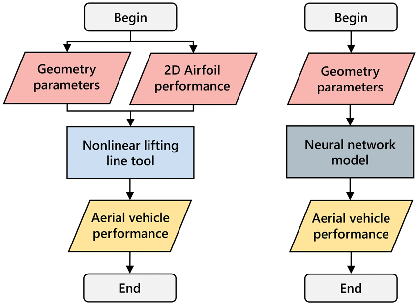
Basic input–output relationships of methodologies.

Figure 2.

ARC UAV and flight tests.⁶

If we focus on aerodynamic analysis applications of such small UAVs, as the complexity of the mathematical model increases, the flow simulation approaches real physical conditions, and the error rate in the analysis decreases. Nevertheless, higher-order solutions generally require extensive computational capacity and time,⁷ making it infeasible for many small UAV design problems. Therefore, in the early phases of aircraft design studies, hundreds of aerodynamic analyses are required for different geometries at particular flow conditions as a part of design optimization. For this reason, it is preferable to use low-order methods, which have a significantly lower computational power requirement and a shorter processing time than the CFD methods based on the Navier–Stokes equations.

Literature review – Computational aerodynamic model

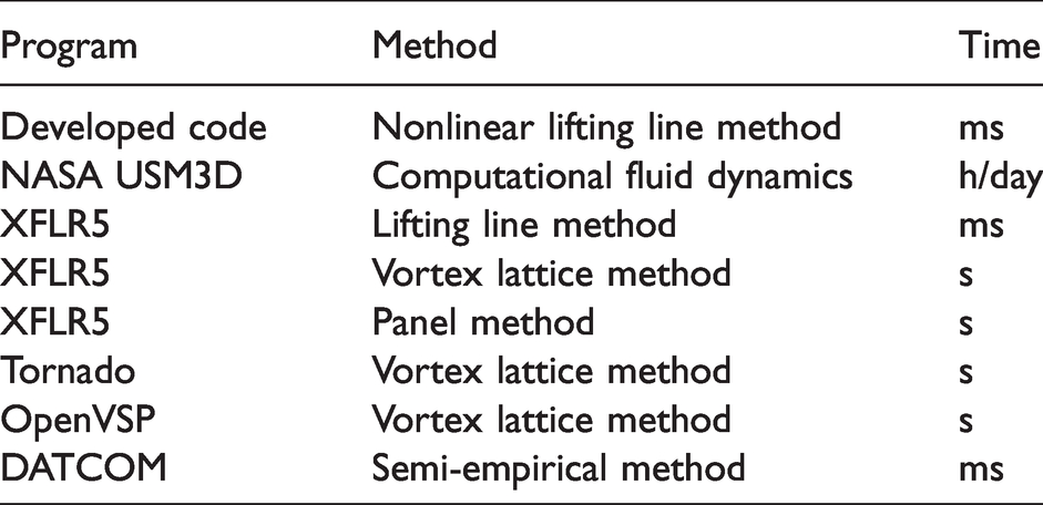
Throughout history, numerous methods are developed for aerodynamic configuration analysis. The early methods have been geared towards hand calculations and the most popular of them is based on the Prandtl’s classical lifting line theory.^8,9 Some of the earlier nonlinear applications of this type of method focused calculation of pre-stall performance of wings.^10,11 Unfortunately, these methods are generally limited with the single lifting surface with no-sweep and no-dihedral at a low and moderate angle of attack flight regime. A discrete application of the lifting line theory named as numerical lifting line method begins with the work of Weissinger.¹² Numerical lifting line methods rely on the assumptions that the flow is irrotational and inviscid.¹³ However, nonlinear applications of this method can also be formed by utilizing the 2D airfoil data^14,15 as the base aerodynamic characteristic model. Another group of methods for aerodynamic configuration analysis, namely lifting surface methods, begins with the work of Falkner.¹⁶ In these methods, any lifting surface is approximated by its camber surface by ignoring the thickness and they are known more like as vortex lattice methods since 1970s. Also, nonlinear applications of this method can be found in the literature.^17,18 Popular computational aerodynamic programs for small and mini UAVs such as XFLR5,¹⁹ OpenVSP/VSPAero,²⁰ Tornado VLM,^21,22 and MachUp²³ utilize these potential theory based methods. When nonlinear analysis of a complete aircraft is considered, it is observed that the estimation success and the reliability of the mentioned studies are limited.^7,24 We further refer the reader to literature^7,24 and Table 4 for an in-depth comparison of the existing computational aerodynamic analysis tools.

Table 4.

Computational aerodynamic analysis tools with their solution time.

Program	Method	Time
Developed code	Nonlinear lifting line method	ms
NASA USM3D	Computational fluid dynamics	h/day
XFLR5	Lifting line method	ms
XFLR5	Vortex lattice method	s
XFLR5	Panel method	s
Tornado	Vortex lattice method	s
OpenVSP	Vortex lattice method	s
DATCOM	Semi-empirical method	ms

State of art and contributions – Computational aerodynamic model

Using potential theory based mathematical models, it is possible to obtain the lift, induced drag, and moment coefficients of a wing at low and medium angles of attack. However, because the viscosity effects in the flow are neglected in potential theory, nonlinear behavior of the lift curve at a high angle of attack and the stall characteristics of the wing in the post-stall region cannot be determined by using low-order linear methods.^25–27 In addition, the maximum lift and viscous drag coefficients, which are important parameters for design, flight control and performance studies,²⁸ cannot be calculated. Nevertheless, in the literature, a number of studies based on low-order methods have been reported that include viscosity effect modifications. For example, in nonlinear applications of the classical lifting line method, viscous effects of the 2D section are reflected to three-dimensional (3D) wing characteristics^11,29 using an iterative method. However, direct application of these methods results in limited and imprecise approximation of the nonlinear aerodynamic characteristics for wing geometries without sweep and dihedral angles in the subsonic regime. As such, our aerodynamic method presented in this work also employs an iterative method, but with a key additional partial linear approximation to the lift curve. Using the new method, we performed a configuration analysis on the Aerospace Research Center (ARC) UAV (see Figure 2) and compared the lift coefficient results with other high- and low-order tools as demonstrated in Figure 3. The results clearly indicate the accuracy of our method in both linear and also nonlinear regimes in comparison to other existing standard tools and methodologies. Further information about this analysis is provided in the “Aerodynamic model” section along with other validation studies. The proposed method brings a novel approach to the literature with the ability to calculate nonlinear aerodynamic performance including the post-stall flight region for a wide class of UAV configurations.

Figure 3.

ARC UAV lift coefficient comparison.

Literature review – AI based aerodynamic model

When the focus is on design and design optimization, traditional engineering tools for the conceptual and preliminary design phases provide limited flexibility and capability in general performance estimation of arbitrary new designs.^30,31 It has been possible to meet these requirements with machine learning methods such as deep learning, which allow us to train a highly nonlinear neural network model through regression analysis via a given set of inputs and associated outputs. There are several studies in the literature on determining the performance of 2D airfoils using machine learning and artificial neural network algorithms.^32–34 It is also known that such algorithms are used to extend the database of a specified aircraft.^35–39 The existing methods within the literature^40–45 such as fuzzy inference systems and neural networks are designed for estimating the performance of a single configuration under a single flight condition and does not contain the complete the aircraft configuration. In addition, these predictions generally focus on a single target coefficient. Thus, the effort is towards functional approximation rather than developing a surrogate model with generalization capability.

State of art and contributions – AI based aerodynamic model

In this work, we focus on the complete aircraft configuration across a wide range of different flight conditions even in the high angle of attack regimes where fully nonlinear behavior is observed. We refer the reader to “Artificial neural network” section, in which we further demonstrate the precision of our approach in comparison to other methods^40,41,45 through direct comparison of the value of the coefficient of determination R². As such, for large-scale design optimization problems, it is necessary to train the model with huge amounts of data that include numerous combinations of different geometric configurations. In the literature, flight tests, experimental studies, and a combination of low- and high-order computational methods have been used to generate restrictive data sets tailored towards more specific design problems.³⁵ Creating large data sets with flight tests, experimental studies, and high-order computational methods such as CFD can become computationally extensive and practically infeasible.⁴⁶ At this stage, low-order computational aerodynamic methods stand out as a cheap and fast option. However, as explained previously, these methods generally do not take into consideration the most critical viscous effects. Therefore, the nonlinear behavior of the lift curve at a high angle of attack and the stall characteristics of the aerial vehicle in the pre- and post-stall regions cannot be determined. Because nonlinear behavior of lift curves is especially seen at low Reynolds numbers, this problem comes to the forefront in every small UAV application. To address this problem, we propose the design of a neural network to predict aerodynamic performance across a wide combination of aerodynamic geometries and configurations. To train the artificial neural network model, a large data set was produced by using our new computationally efficient nonlinear lifting line method. Because of the speed and reliability of the aerodynamics analysis tool, it was possible to generate and analyze tens of thousands of configurations in minutes even on a personal computer. The designed artificial neural network model essentially calculates the aerodynamic performance of various UAV configurations including the 3D maximum lift coefficient and pre- and post-stall aerodynamic behavior without requiring 2D airfoil performance data. In the training of the neural network model, the NACA four-digit series airfoils are defined by their geometric parameters: camber location, camber, and thickness ratio.⁴⁷ This definition allows the model to use only the dimensional parameters as inputs without requiring 2D airfoil performance data. The results show that model prediction exhibits an almost 1-1 coincidence with the numerical data even for configurations with different airfoils that are not used in model training. This demonstrates the generalization capability of the trained model. This is further illustrated in Figure 4, in which the lift coefficient prediction from the neural network model shows an excellent match with the real lift coefficient data associated with a conventional UAV configuration. Further information and test cases can be found in the “Application of surrogate model” subsection.

Figure 4.

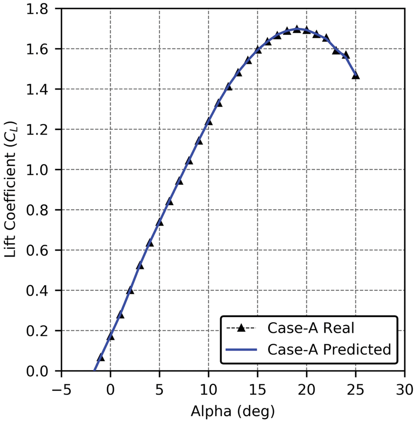
Neural network predictions for lift coefficient of a conventional UAV.

The results presented in this article partially originate from two preliminary works^5,7 from our research group. To be specific, the aerodynamic model part partially covers the research in Karali et al.⁷ However, in this study, we have further developed the existing algorithm and employed a more systematic approach by incorporating the fuselage aerodynamics into the analysis tool so that it can model the complete UAV aerodynamics. In addition, we have reduced the number of iterations required to achieve the final circulation distribution required by updating the iteration section of the algorithm. The origin of the neural network model in the second part of this work stems from our preliminary analysis in Karali et al..⁵ In this article, we have extended the methodology from Karali et al.⁵ to a complete UAV solution by adding the fuselage definition to the AI model. In addition, we have significantly enlarged the data set used to train of the model. Based on these differences, we have produced a new feature set using a novel algorithm and developed a new network structure. This was crucial for claiming generalization capability for the proposed method and model. In addition, in this work, we have demonstrated the capability of the model through a simple illustrative design optimization example.

The rest of the article is organized as follows: In the “Aerodynamic model” section, the nonlinear lifting line method is explained, providing insight into its mathematical basis and several test examples. In the “Artificial neural networks model” section, in-depth information is given about the structure of the algorithm, data sets, and test examples. Next, the surrogate model used in the design optimization of a small UAV and the results are provided. Finally, the conclusions are presented, and the objectives planned to be achieved in future studies are explained.

Aerodynamic model

As the basis of our aerodynamic configuration analysis, we utilize our nonlinear lifting line approach,⁷ which modifies the potential flow based Prandtl’s lifting line theory for the calculation of nonlinear characteristics at high angles of attack. In Figure 5, the process diagram of the nonlinear lifting line methodology is given. The main features of the method can be summarized as a partial linear approximation to the lift curve and an iteration process to correct the error due to linear approximation. Calculations in the method begin from the zero lift angle of attack of 3D wing geometry and proceeds step by step with an appropriate increase in the angle of attack. At each angle of attack, the error in the lift coefficient due to linear approximation is corrected by using an iteration process on a spanwise circulation distribution.

Figure 5.

Flowchart of nonlinear lifting line methodology.

Classical lifting line theory

In Prandtl’s lifting line theory, also known as classical lifting line theory, the flow around a finite wing is simulated by a system of horseshoe vortices in uniform parallel free flow. The leading edge filaments of the horseshoe vortex all coincide on the wing as the bound vortex to represent the effect of the wing, while the side part filaments reflect the impacts of the trailing vortices. Detailed information about this mathematical model can be found in any aerodynamics textbook.^48,49

In general applications of this model, the streamwise variation in strength of the bound vortex is represented by the sinus Fourier series

Γ (θ) = 4 s V_{\infty} \sum_{j = 1}^{N} A_{j} \sin (j θ)

(1)

and the aerodynamic parameters of the lifting surface are obtained as follows

C_{L} = π A R A_{1}

(2)

C_{D_{i}} = \frac{C_{L}^{2}}{π A R} (1 + δ); δ = \sum_{j = 2}^{N} j {(\frac{A_{j}}{A_{1}})}^{2}

(3)

ε = \sum_{j = 1}^{N} \frac{j A_{j} \sin (j θ)}{\sin (θ)}

(4)

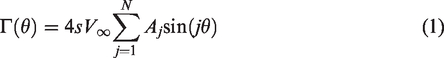
The Fourier coefficients, A_j, depend on the geometry of the wing and the angle of attack. In the classical method, a linear solution is obtained for the 3D wing with a one-step calculation using the linear lift curve slope of the 2D profile. However, in this article, a new partial linear approach is used for the 2D lift curve.

Partial linear approach to nonlinear lift curve

In the nonlinear region of a lift curve, for a spanwise station, i, of a wing at any incidence, let $α_{i}^{k}$ and $c_{l_{i}}^{k}$ be the local geometric angle of attack and the local lift coefficient, respectively (see Figure 6). Assume that the lift curve slope remains constant for a small increase of $Δ α$ in the angle of attack. If the new local geometric angle of attack is defined as $α_{i}^{k + 1}$ , then the new lift coefficient is obtained as

c_{l_{i}}^{k + 1} = c_{l_{i}}^{k} + a_{i}^{k} (α_{i}^{k + 1} - α_{i}^{k})

(5)

Figure 6.

Partial linear approach to the lift curve.

For the same lift coefficient, the following equation can be written with a 2D approach as in the classical lifting line method

c_{l_{i}}^{k + 1} = c_{l_{i}}^{k} + a_{\infty_{i}}^{k} (α_{e_{i}}^{k + 1} - α_{e_{i}}^{k})

(6)

where α_e is the effective angle of attack and

α_{\infty}

is the 2D lift curve slope, which is also assumed constant for the increase

Δ α

. The differences between the local geometric angles of attack and the effective angles of attack are the downwash angles

α_{i}^{k} - α_{e_{i}}^{k} = ε_{i}^{k}; α_{i}^{k + 1} - α_{e_{i}}^{k + 1} = ε_{i}^{k + 1}

(7)

Introducing these relations in equation (6)

c_{l_{i}}^{k + 1} = c_{l_{i}}^{k} + a_{\infty_{i}}^{k} [(α_{i}^{k + 1} - ε_{i}^{k + 1}) - (α_{i}^{k} - ε_{i}^{k})]

(8)

Recalling that the change in the angle of attack $Δ α$ is

α_{i}^{k + 1} - α_{i}^{k} = Δ α

(9)

the following equation is obtained

c_{l_{i}}^{k + 1} = c_{l_{i}}^{k} + a_{\infty_{i}}^{k} [Δ α - (ε_{i}^{k + 1} - ε_{i}^{k})]

(10)

If the Kutta–Joukowski theorem for the lift is applied, the section lift coefficient is obtained in terms of the circulation

L^{'} = ρ_{\infty} V_{\infty} Γ = c_{l} \frac{1}{2} ρ_{\infty} V_{\infty}^{2} c \to c_{l} = \frac{2 Γ}{V_{\infty} c}

(11)

Introducing this relation, equation (10) gives

\frac{2 Γ^{k + 1}}{V_{\infty} c_{i}} = \frac{2 Γ^{k}}{V_{\infty} c_{i}} + a_{\infty_{i}}^{k} [Δ α - (ε_{i}^{k + 1} - ε_{i}^{k})]

(12)

Introducing equations (1) and (4), which represent the circulation and the downwash angle in terms of the Fourier coefficients, into equation (12) and rearranging, one obtains

\sum_{j = 1}^{N} (\frac{1}{μ_{i}^{k}} + \frac{j}{\sin θ_{i}}) \sin j θ_{i} A_{j}^{k + 1} = \sum_{j = 1}^{N} (\frac{1}{μ_{i}^{k}} + \frac{j}{\sin θ_{i}}) \sin j θ_{i} A_{j}^{k} + Δ α

(13)

where

μ_{i}^{k} = \frac{8 s}{a_{\infty_{i}}^{k} c_{i}}

(14)

Thus, the relation between the spanwise circulation distribution and wing geometry is ensured. Applying this equation to properly distributed N sections (called stations) along the wingspan, the following linear equation system is obtained

\sum_{j = 1}^{N} D_{i j}^{k} A_{j}^{k + 1} = \sum_{j = 1}^{N} D_{i j}^{k} A_{j}^{k} + Δ α, (i = 1, \dots, N)

(15)

where

D_{i j}^{k} = (\frac{1}{μ_{i}^{k}} + \frac{j}{\sin θ_{i}}) \sin j θ_{i}

(16)

This system of equations can be written in matrix form as follows

[D_{i j}^{k}] {A_{j}^{k + 1}} = [D_{i j}^{k}] {A_{j}^{k}} + {Δ α}

(17)

where

A_{j}^{k}

are the Fourier series coefficients of the previous angle of attack, and they are assumed to be known previously. The solution of this system of equation is defined as

{A_{j}^{k + 1}} = {A_{j}^{k}} + {[D_{i j}^{k}]}^{- 1} {Δ α}

(18)

By using the obtained $A_{j}^{k + 1}$ Fourier coefficients, the aerodynamic parameters of the wing such as the lift coefficient, induced drag coefficient, and effective angle of attack can be calculated for the new step. It should be noted that, at each new angle of attack step, the effective angles of attack and 2D lift curve slope, $a_{i}^{k}$ , and therefore, the $D_{i j}^{k}$ coefficients, will change.

When equation (18) is examined, it appears that each calculation step depends on the previous solution. Thus, it is necessary to determine a starting point at the beginning of equation (18). In this study, the zero lift angle of attack of the 3D wing was used as the beginning of the solution. The procedure to obtain this angle is given in the next subsection.

Moreover, as can be seen from equation (18), the partial linear approach solution depends on the step size $Δ α$ . Using a rectangular planform wing with an AR 10 and NACA 4415 cross section, a test application was conducted and the results are demonstrated in Figure 7. It can be clearly stated that the different step sizes in the calculations lead to different results in 3D wing performance.

Figure 7.

Calculated lift curves for different step sizes using equation (18).

In Figure 7, as the calculation steps become smaller, the solutions begin to converge to a single specific curve. However, it is not practical to analyze with very small step sizes. To overcome this problem, after each calculation step, an iterative procedure is applied to the spanwise circulation distribution. The detailed information about this process is given in the section titled “Iteration method for circulations”. However, first, the Fourier series of the starting point must be calculated.

Calculation of zero lift angle of attack

If the lift curve of a 3D wing is examined, it is observed that the zero lift angle of attack point usually remains in a narrow linear region. It is possible to find this angle by an inverse solution using classical lifting line theory. To achieve this, first, the system of linear equations is arranged in matrix form as follows

[D_{i j}] {A_{j}} = {α_{i} - α_{0_{i}}}

(19)

where

α_{0_{i}}

is the zero lift angle of attack of the ith section along the span, and

D_{i j}

is given above by equation (16). If there is a geometric twist on the wing, it is convenient to define local geometric angles of attack in terms of the root section’s angle of attack, α_root, and the local twist angle β_i as follows

α_{i} = α_{root} + β_{i}

(20)

With this definition, equation (19) takes the form

[D_{i j}] {A_{j}} = {α_{root}} + {β_{i} - α_{0_{i}}}

(21)

As is known from classical lifting line theory, the lift coefficient depends on the first Fourier coefficient A₁ as given in equation (2), and it is clear that, when the lift is zero, A₁ is also zero. Thus, if equation (21) is rearranged with α_root as the unknown instead of A₁, the following system of linear equations is obtained

[\begin{matrix} - 1 & D_{12} & \dots & D_{1 N} \\ - 1 & D_{22} & \dots & D_{2 N} \\ ⋮ & ⋮ & ⋮ & ⋮ \\ - 1 & D_{N} & \dots & D_{N N} \end{matrix}] {\begin{matrix} α_{root} \\ A_{2} \\ ⋮ \\ A_{N} \end{matrix}} = {\begin{matrix} β_{1} - α_{0_{1}} \\ β_{2} - α_{0_{N 2}} \\ ⋮ \\ β_{N} - α_{0_{N}} \end{matrix}}

(22)

In this matrix system, the RHS vector is known from the geometrical properties of the wing. The $D_{i j}$ coefficients are calculated by using the 2D lift curve slope $a_{\infty}$ of the airfoil around its zero lift angle of attack.

Iteration method for circulations

In the step-by-step procedure explained in the partial linear approach, the Fourier coefficients at any new angle of attack are calculated by using 2D lift curve slopes at the previous angle of attack. Because these slopes are assumed to be the same as the values at the previous angle of attack for the one-step calculation, the Fourier coefficients calculated for the new angle of attack have an error depending on the step size $Δ α$ . Because of the iteration process, which is shown with the red dashed line in Figure 8, the error is minimized. These errors have been shown in Figure 7 for several step sizes, and it is seen that while the step size is larger, the error is also larger. Therefore, an iteration is required at each angle of attack step to correct this error.

Figure 8.

Iteration process representation on the lift curve.

The iterative method used in the current study is based on the correction of the spanwise circulation distribution by using the wing section’s 2D lift coefficients obtained either experimentally or numerically. This procedure begins with the wing lift coefficient obtained at the new angle of attack using the partial linear approach.

The iteration steps are as follows:

(i) Calculate the circulation distribution by using the Fourier coefficients obtained from the partial linear approximation

Γ_{i}^{old} = 4 s V_{\infty} \sum_{j = 1}^{N} A_{j} \sin j θ_{i}

(23)

(ii) Calculate the downwash angles by using the Fourier coefficients in equation (4) and the effective angles of attack as follows

α_{e_{i}} = α_{i} - ε_{i}

(24)

(iii) For each section, determine the local lift coefficient by using the effective angles of attack in the section’s 2D data obtained either experimentally or numerically.

(iv) Calculate the new circulation distribution with the following relationship obtained from the Kutta-Joukowski law for the lift and the lift coefficient definition

Γ_{i}^{new} = \frac{1}{2} V_{\infty} c_{i} c_{l_{i}}

(25)

(v) Compare these circulations with the previous one. If the difference is smaller than $10^{- 5}$ , exit the iteration loop, otherwise calculate new circulation values as follows

Γ_{i} = Γ_{i}^{old} + R F (Γ_{i}^{new} - Γ_{i}^{old})

(26)

where RF is a relaxation factor, whose value is chosen as 0.05 here in the examples

(vi) Reorganizing equation (1) as a system of linear equations, one obtains

[\begin{matrix} \sin 1 θ_{1} & \sin 3 θ_{1} & \dots & \sin n θ_{1} \\ \sin 1 θ_{2} & \sin 3 θ_{2} & \dots & \sin n θ_{2} \\ ⋮ & ⋮ & ⋮ & ⋮ \\ \sin 1 θ_{n} & \sin 3 θ_{n} & \dots & \sin n θ_{n} \end{matrix}] {\begin{matrix} A_{1} \\ A_{2} \\ ⋮ \\ A_{n} \end{matrix}} = {\begin{matrix} Γ_{1} / 4 s V_{\infty} \\ Γ_{2} / 4 s V_{\infty} \\ ⋮ \\ Γ_{n} / 4 S V_{\infty} \end{matrix}}

(27)

In equation (27), the coefficient matrix comprises constant and known parameters. Because the circulation distribution is obtained in the previous step, calculate new Fourier coefficients using the inverse of coefficient matrix.

(vii) Repeat steps 1 to 6 until convergence is obtained.

A case study of this iteration process is conducted on the wing that was used above to generate Figure 7. The outcome is shown in Figure 9 together with the previous lift curves. The results of this application obtained for $Δ α = 2 °$ and $Δ α = 5 °$ steps demonstrate the capability of the iteration method.

Figure 9.

Lift curves for different step sizes of the rectangular wing.

Figure 10.

U.S. Navy RQ-2B Pioneer⁵¹ and RQ-7B Shadow.⁵²

Calculation of aerodynamic coefficients

Using the final form of the Fourier series coefficients, it is possible to calculate the lift and induced drag coefficients via equations (2) and (3). However, the classical methodology does not give information about any other force or moment parameters. Nevertheless, the viscous drag and pitching moment coefficients can be obtained by using 2D experimental or numerical data of the wing section. To achieve this, first 2D data are interpolated to obtain corresponding values for the effective angles of attack given by the method at each spanwise station. Later, these values are integrated numerically along the span as in equations (28) and (29)

C_{D_{v}} = \frac{2}{S} \sum_{i = 1}^{N} S_{i} {\bar{c}}_{D_{v_{i}}}; {\bar{c}}_{D_{v_{i}}} = \frac{c_{D_{v_{i}}} + c_{D_{v_{i + 1}}}}{2}

(28)

C_{m_{y}} = \frac{2}{S \bar{c}} \sum_{i = 1}^{N} S_{i} {\bar{c}}_{i} {\bar{c}}_{m_{y_{i}}}; {\bar{c}}_{m_{y_{i}}} = \frac{c_{m_{y_{i}}} + c_{m_{y_{i + 1}}}}{2}

(29)

where

S_{i} = \frac{c_{i} + c_{i + 1}}{2} (y_{i + 1} - y_{i}) and {\bar{c}}_{i} = \frac{c_{i} + c_{i + 1}}{2}

(30)

Similar to these coefficients, flow separation points and pressure coefficients can be also calculated by using 2D data of the wing section. The data in the look-up table are interpolated according to the effective angle of attack at each spanwise station.

Application of the aerodynamic model

In this section, the results of several test applications of the new nonlinear lifting line method are presented to show its applicability, limits, advantages, and disadvantages. Using the Visual Basic programming language, a computer program was developed. The main algorithm of the program is shown in Table 1.

Table 1.

Algorithm of nonlinear lifting line method.

Algorithm of N-LLT program
Inputs:
Geometry parameters
2D Airfoil performance data
1: for $i = 1 t o N \leftarrow$ number of stations
2: compute geometry parameters ${c (i), y (i), \dots}$
3: end for
4: solve $[D_{i j}] {A_{j}} = {α_{root}} + {β_{i} - α_{0_{i}}}$
5: while $α_{root} < α_{max} \leftarrow$ max AoA limit
6: ${A_{j}^{k + 1}} = {A_{j}^{k}} + {[D_{i j}^{k}]}^{- 1} {Δ α}$
7: $Γ_{i}^{old} = 4 s V_{\infty} \sum_{j = 1}^{N} A_{j} \sin j θ_{i}$
8: for $iter = 1 t o maxiter$
9: compute $A_{j}$ using Γ _i
10: $ε = \sum_{j = 1}^{N} \frac{j A_{j} \sin (j θ)}{\sin (θ)} \leftarrow$ downwash angle
11: $α_{e_{i}} = α_{i} - ε_{i}$
12: $Γ_{i}^{new} = \frac{1}{2} V_{\infty} c_{i} c_{l_{i}}$
13: if $\| Γ_{i}^{old} - Γ_{i}^{new} \| < 10^{- 5}$
14: exit for
15: end if
16: $Γ_{i} = Γ_{i}^{old} + R F (Γ_{i}^{new} - Γ_{i}^{old})$
17: end for
18: compute $C_{L}, C_{D}, C_{m}$
Output:
Aerodynamic performance of 3 D geometry

First, the method was validated with experimental data. Ostowari and Naik’s experimental studies on NACA 44XX airfoil sections are convenient data sources for the validations.⁵⁰ These studies include 2D experimental data for NACA 44XX airfoils for different thickness ratios as well as 3D experimental results for rectangular wings of different aspect ratios at several Reynolds numbers. These airfoils are well known and very popular in aviation. In particular, several UAVs, micro aerial vehicles, and light aircraft use these four-series wing sections. As such, even tactical UAVs such as AAI RQ-7 Shadow and AAI RQ-2 Pioneer are examples of UAVs with their NACA 4415 cross-sectional rectangular wings.

Hence, a rectangular wing of aspect ratio 9 with a NACA 4415 section is chosen for the first test case (see Table 2). This wing will be analyzed for two different Reynolds numbers: $0.25 \times 10^{6}$ and $0.50 \times 10^{6}$ . In the next figures, M was used in the legends to represent the Reynolds number 10⁶.

Table 2.

Test Case I specifications.

Section	Planform	AR	Re
NACA 4415	Rectangular	9	$0.25 \times 10^{6}$ – $0.50 \times 10^{6}$

The results obtained from the analysis are illustrated together with the experimental data in Figure 11. It is clearly observed that the numerical results are almost 1-1 coincident with the experimental data in both the linear and nonlinear regions. The calculated maximum lift coefficients are nearly equal to the experimental values for both Reynolds numbers. These results show that the current method can precisely calculate the lift coefficient in both the linear and nonlinear regions up to $10 °$ beyond the stall point for $R e = 0.25 M$ . However, after the $25^{°}$ angle of attack, there is a small offset between the lift curves for $R e = 0.50 M$ . Furthermore, the calculated total drag and pitching moment curves also showed satisfactory results. It must be noted that the results, which are taken from the literature, are represented by an average curve, because some fluctuations are present in the experimental data of the pitching moment coefficients.

Figure 11.

Test Case I: lift, total drag, and pitching moment coefficients.

In the second test case, a rectangular wing of aspect ratio 12 with a NACA 4415 section was used (see Table 3). In comparison with Test I, the only difference in this case is that the aspect ratio has been slightly increased.

Table 3.

Test case II specifications.

Section	Planform	AR	Re
NACA 4415	Rectangular	12	$0.25 \times 10^{6}$ – $0.50 \times 10^{6}$

As in the previous test case, numerical results are given with validation data in Figure 12. In this example, the nonlinear behavior of the experimental lift curve begins at a nearly $12 °$ angle of attack. As in the previous test case, the numerical method is able to calculate this nonlinear region accurately up to a $25 °$ angle of attack. As seen in Figure 12, the developed method can predict the post-stall aerodynamic behavior of the 3D wing. The second graph shows the results of the calculated total drag coefficient for a zero lift angle attack up to $α = 30 °$ . These numerical results are compared with the experimental data in the literature. From this information, it is clear that the value of the total drag coefficient calculated using the method is very close to its experimental value. In the third graph, the numerical pitching moment results exhibit an offset relative to the experimental data. Nevertheless, the method estimates the behavior of the moment curve with a small margin of error.

Figure 12.

Test Case II: lift, total drag, and pitching moment coefficients.

In the next validation study, the developed tool will be compared with other computational aerodynamic tools. Several tools have been described in the literature for aerodynamic analysis of lifting surfaces and configurations. The tools used in this study are listed in Table 4 with their running time. In this table, all tools except NASA TetrUSS USM3D⁵³ are freely downloadable analysis tools.

In this test case, the geometry is a rectangular wing of AR = 12 with a NACA 4415 section. The analyses for this case were performed for a Reynolds number of 3 million based on the chord length. Specifications for geometry are given in Table 5. Two-dimensional data for the current developed method are taken from a database in the literature⁵³ generated by using NASA USM3D tool.

Table 5.

Test Case III specifications.

Section	Planform	AR	Re
NACA 4415	Rectangular	12	$3.0 \times 10^{6}$

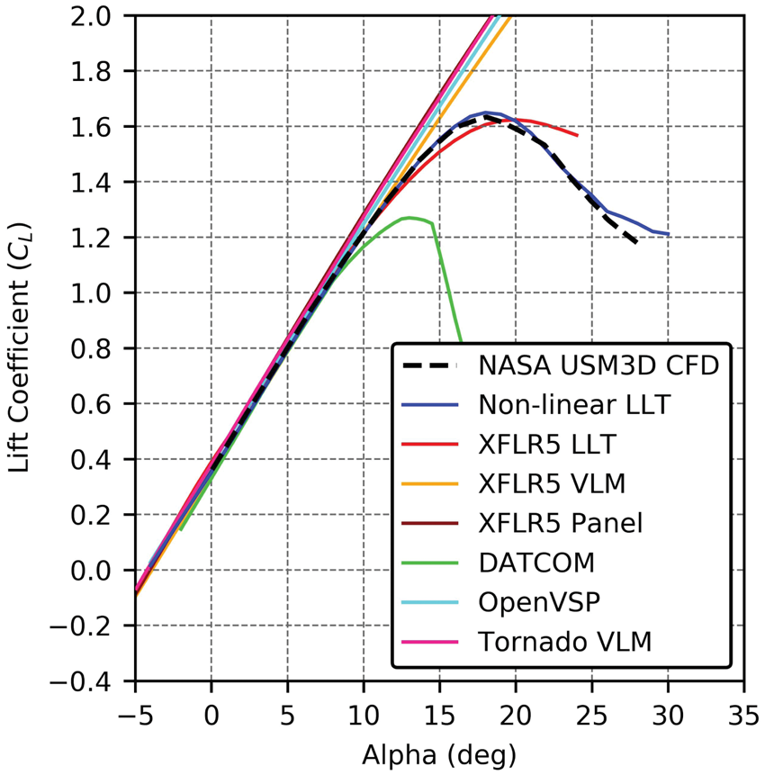
The results of all these analyses are presented in Figure 13. In the figure the black dashed line represents 3D data obtained using the NASA USM3D CFD tool and given in a database in the literature.⁵³ XFLR5 VLM,¹⁹ XFLR5 Panel Method,¹⁹ OpenVSP (VSPAero) VLM, and Tornado VLM²² codes calculate the lift curves with a linear approximation because their mathematical model is based on potential theory. Hence, these tools are not able to predict the maximum lift coefficient and nonlinear behavior in the pre- and post-stall regions. On the other hand, XFLR5 LLT (only for a single surface) and DATCOM perform a calculation to estimate the maximum lift coefficient. However, the DATCOM prediction results in particular are far from satisfactory, as seen in Figure 13.

Figure 13.

Test Case III: lift coefficients.

A detailed examination of Figure 13 shows that the developed method calculated both the linear and nonlinear region of the lift curve with a minimum error margin. Further, the calculated maximum lift coefficient almost equals validation value.

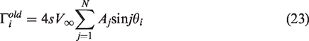
In Figure 14, the section lift coefficients, which are calculated by the developed method, are compared with the CFD results. Considering that the nonlinear behavior starts at 12°, the calculated lift distribution at the pre-stall angle of attack ( $α = 14 °$ ) appears to be highly accurate. It is important to note that the method calculates these values at a low number of stations. This is why lines connecting these points perfectly straight. In addition to this, nonlinear LLT predicts the lift distribution with a very small error margin at the stall angle of attack, which is represented by the orange line. Furthermore, it can calculate the general characteristics of the lift distribution in the post-stall region correctly. As can be seen from the red curve, a large fluctuation in the lift distribution can be captured by the developed method. However, low fluctuations between the spanwise stations are ignored by the program. The program can calculate all the angles of attack range within 0.06 s on a typical personal computer configuration.

Figure 14.

Test Case III: section lift coefficient distributions.

The flow separation lines, which is another feature calculated by the developed method, are compared with the results in the database. For this purpose, the required 2D flow separation input was obtained by using XFOIL. The results, shown in Figure 15, are formed as a scaled half-wing. In the graphs, the same color was used for the angles of attack as in the previous ones. According to the lift curve in Figure 13, wing stall begins at an 18° angle of attack. It is generally known that for a rectangular planform, the wing’s root region stalls first. This situation can also be observed in the results of the numerical analysis and CFD. Similar to the lift distribution, the method was also able to capture large changes in the flow separation points at the spanwise stations. The results were found to be quite successful for a low-order method.

Figure 15.

Test Case III: flow separation points.

Extension of the method to aerodynamic analysis of the conventional aerial vehicle

It is known that the Prandtl’s classical lifting line theory is applicable only to a single lifting surface. In this study, a methodology was developed to make it possible to solve lifting surface configurations. To accomplish this, it is necessary to calculate the downwash of the wing on the tail. A nonlinear methodology can be repeated for the aft surface. In Phillips et al.,⁵⁴ a mathematical model is developed to estimate the downwash a few chord lengths or more aft of an unswept wing. In this model, a rolled-up vortex sheet is taken as a single horseshoe shaped vortex filament. A numerical calculation is performed with Fourier series coefficients and wing geometry data; therefore, completely arbitrary spanwise variations can be used in the method.

Downwash velocities at tail stations can be calculated with Fourier coefficients of the wing geometry, which is obtained at the end of the iteration process. In equation (31), the k_b, k_p, and k_v parameters represent the wingtip vortex span, tail position, and wingtip vortex strength factors, respectively. While the dimensionless parameters k_v and k_b depend on the planform shape of the wing, k_p depends on both the planform shape of the wing and the position of the tail relative to the wing

ε_{i} (\bar{x}, \bar{y}, \bar{z}) ≅ \frac{- V_{z} (\bar{x}, \bar{y}, \bar{z})}{V_{\infty}} = \frac{k_{v} k_{p}}{k_{b}} (C_{L_{w}} / A R_{w})

(31)

If the downwash angle at the tail location and twist angle of the tail are known, the angle of attack for each tail station is obtained as

α_{{tail}_{i}} = α_{root} + β_{{tail}_{i}} - ε_{i}

(32)

With this information, the new developed nonlinear lifting line method can be applied to the tail geometry. Thus, all the calculated parameters related to the wing are obtained for the tail as well, and nonlinear analysis of the wing-tail configurations becomes possible. The aerodynamic force coefficients for the lifting surface configurations are obtained as in equations (33) and (34)

C_{L_{total}} = C_{L_{wing}} + C_{L_{tail}} \frac{S_{tail}}{S_{ref}}

(33)

C_{D_{total}} = C_{D_{wing}} + C_{D_{tail}} \frac{S_{tail}}{S_{ref}}

(34)

In this way, it is possible to calculate the total drag of wing-tail configurations with viscous effects. However, it is known that the fuselage geometry has a major impact, especially in terms of parasitic drag for the complete configuration. According to Sadraey, usually 30–50% of the aircraft’s zero lift drag ( $C_{D_{o}}$ ) is caused by the fuselage.⁵⁵ As in the example used in this study, UAVs typically have simple fuselage geometries. Hence, it is possible to calculate the drag force using analytical/empirical methods.

Using these methods,⁵⁶ zero-lift drag coefficient for fuselage geometries can be formulated as

C_{D_{0_{fslg}}} = R_{w f} C_{f} {1 + \frac{60}{{(l_{f} / d_{f})}^{3}} + 0.0025 (l_{f} / d_{f})} \frac{S_{w e t_{fslg}}}{S_{ref}}

(35)

In addition to this coefficient, other components such as landing gears, stores, and pylons can be calculated with these analytical/empirical methods. In light of this information, the total drag coefficient of the aircraft can finally be calculated with equation (36)

C_{D_{total}} = C_{D_{wing}} + C_{D_{tail}} + C_{D_{fuselage}} + C_{D_{misc}}

(36)

In a simple UAV analysis, the pitching moment is needed to determine the static stability of the vehicle. If a component-based approach is used to calculate this coefficient, equation (37) is obtained

C_{m_{total}} = C_{m_{c g_{wing}}} + C_{m_{c g_{tail}}} + C_{m_{c g_{fuselage}}}

(37)

The contribution of the wing and tail to an airplane’s static stability can be calculated with the basic force–moment equations that determine total moment over the CG point. Multhopp’s method can be used to calculate the contribution of the body to the pitching moment⁵⁷

C_{m_{0_{fuselage}}} = \frac{k_{2} - k_{1}}{36.5 S \bar{c}} \sum_{x = 0}^{x = l_{f}} w_{f}^{2} (α_{0_{w}} + i_{f}) Δ x

(38)

C_{m_{α_{fuselage}}} = \frac{1}{36.5 S \bar{c}} \sum_{x = 0}^{x = l_{f}} w_{f}^{2} \partial ε_{u} / \partial α Δ x

(39)

Detailed information and sample applications about these equations can be found in the literature.^56,57 Thus, all the equations necessary for a complete UAV analysis are completed.

The new developed tool has been used in the design and mathematical modeling of the ARC UAV (see Figure 16). To be specific, using the proposed methodology, the nonlinear performance of different UAV configurations was analyzed and the results quickly transferred to the dynamic model for simulation and flight control system design. We refer the reader to the literature^58–60 for further details of usage of these models within the calculation of stability derivatives and the flight control system design processes.

Figure 16.

ARC UAV geometry.

In this example, the aerodynamic performance of the project UAV was compared with various analysis tools, and the results are presented in Figure 17. Inspection of the lift curve shows that the method is in good agreement with the CFD (ANSYS Fluent) results in both the linear and nonlinear regions, including stall behavior. Using identical computational hardware configuration, the Fluent CFD analysis for the $C_{L} - α$ calculation for 15 test points took 120 h, whereas the new developed methodology took 0.01 s to compute the $C_{L} - α$ calculation for 30 test points. This shows the remarkable computational advantage that can be obtained by using the proposed method while capturing all the important nonlinear effects. Consequently, the proposed methodology has the potential to serve as a rapid configuration analysis tool for both stand-alone analysis and multidisciplinary design optimization schemes.

Figure 17.

Test Case IV: lift, total drag, and pitching moment coefficients.

In the second graph of Figure 17, the total drag coefficient curves are compared. As in Test Case III, the VLM program’s induced drag results are summed with their viscous drag module solutions. In the developed method, the contribution of the fuselage to the total drag coefficient was added to the results obtained directly from the lifting surfaces.

The angle of attack limit that XFLR5 converges to in viscous analysis lies in a very narrow range for this configuration. The developed method exhibits comparable results with CFD and Tornado up to the $9^{°}$ angle of attack. Interestingly, there is a reduction in the rate of increase of CFD results after this point. The DATCOM results are not very reliable in terms of drag, as stated in the user manual warnings.⁶¹ Figure 17 shows that there is a large offset in the drag curve. This situation also dictates that DATCOM should be used carefully considering the limits in empirical tables, especially for UAV dimensions and flight regimes.

Finally, Figure 17 compares the pitching moment curves. As shown in the figure, the computational tools’ results are compatible with each other. However, the developed method, which is shown with a blue line, exhibits significantly different results at higher angle of attack regimes as it calculates the pitching moment curve with fully nonlinear behavior. Detecting this behavior is critical to accurately model and control the UAV in agile flight. Because the CFD data are missing in this figure, the offset in the calculation of the developed method has been tested in a different way. To show that the difference in behavior is caused by the inherent nonlinear structure of the lift curve, linear inviscid 2D performance inputs were used. This analysis is represented with a black dashed line, and it is clear that the results are consistent with those from the other analysis tools. In this way, it can be concluded that viscous effects are the main reason for the variation exhibited by the developed method compared to the other tools. In the next section, we focus on generating an efficient aerodynamic configuration analysis engine that can be utilized for design optimization of small UAVs.

Artificial neural network model

One of the key challenges towards in design optimization of small UAVs is the lack of fast and precise aerodynamic configuration analysis engines that can be utilized as part of the optimization routines. Toward this goal, in this work, we generate a black-box function that can predict the aerodynamic characteristics of UAV configurations including viscous effects by using deep learning techniques. To be specific, an artificial neural network architecture is designed and trained using the data set created by the aerodynamic analysis tool presented in the previous section.

Figure 18 shows the colorized process diagram of the artificial neural network methodology. Extending our previous work,⁵ the contribution of the fuselage to the total drag and pitching moment coefficients is incorporated into the model by expanding the data set. In addition, improvements have been made to both the feature set and the network structure of the method. Through this, we have achieved a wider generalization capability within the design space. With the increase in the training data size, the accuracy of the neural network in estimating aerodynamic performance increases. In the next subsections, we step by step follow the process diagram of the artificial neural network methodology shown in Figure 18, starting with data generation. All the data sets, features, and training configurations are given in detail to ensure the reproducibility of the presented results.

Figure 18.

Flowchart of artificial neural network model.

Data generation

Our nonlinear lifting line method offers a fast and reliable method for creating the aerodynamic data necessary to train the neural network model. Toward creating the base geometric aerodynamic data set, the geometry definition was modified, and multiple XFOIL⁶² analysis outputs were used as the 2D performance input. Each configuration was analyzed for approximately 30 different angles of attack. The relationship between calculation time and configuration numbers is shown in Figure 19 with a log-log scale. The calculation times show a strong first-order (i.e., n = 1) log relationship. It is also important to note that in this study, a personal computer is used as the main computational environment.

Figure 19.

Relationship between the number of configurations and the calculation time.

In this study, the final data set with 94,500 configurations was used, but this number can be increased with various geometric combinations. Table 6 shows the number of configurations and the total number of rows in the data set.

Table 6.

Data set dimensions and generation times.

Number of configurations	Total row number	Parameters (columns)	Run time (min)
94,500	2,835,000	25	17.5

Table 7 summarizes all the 25 parameters in the data set. Here, 21 of them are related to geometry, while 1 parameter is related to the flow condition, and 3 to the performance outputs.

Table 7.

All configuration parameters in data set.

Wing and tail parameters

Span

Root chord length

Tip chord length

Incidence angle

Airfoil thickness ratio

Airfoil camber ratio

Airfoil max. camber location

2D performance input file name

Fuselage

Hydraulic diameter

Length

Location

x-Distance

y-Distance

z-Distance

Flow condition

Angle of attack (α)

Performance coefficients

Lift coefficient (C_L)

Drag coefficient (C_D)

Pitching moment coefficient (C_m)

In the first stage of the study, certain geometrical limits were determined to prevent the data size from increasing too much. However, as mentioned in the previous sections, it will not be difficult to increase these combinations because the program can solve one configuration for 30 different flow conditions in 0.01 s. The parameters determined for the combinations are listed in Table 8.

Table 8.

Geometric parameters and ranges in the data set.

Surface	Airfoil	Chord	AR	Incidence	x-Location	Reynolds number
	NACA 2412
Wing	NACA 4412	0.2 to 0.6	10 to 20	−2 to 2	–	$0.4 \times 10^{6}$ to $1.2 \times 10^{6}$
	NACA 6412
Tail	NACA 0012	$(0.5 t o 1) * c_{wing}$	4 to 8	−2 to 2	$(0.4 to 0.6) \times b_{wing}$	$0.2 \times 10^{6}$ to $1.2 \times 10^{6}$

Whereas different camber ratio profiles are used in the wing sections, the tail profile is restricted to the symmetrical NACA 0012 profile. The Reynolds number depending on the wing mean aerodynamic chord was determined to be equivalent to the flight regime of the small UAVs. By configuring the geometric dimensions and positions of the tail and fuselage to the wing geometry, numerous different configurations with logical dimensions have been produced.

Feature extraction

In the feature extraction process, first, the initial data set of the raw data is examined. For this purpose, the correlation matrix was calculated using Pearson’s method. In Figure 20, positive correlations between features are shown with dark blue and negative correlations with light blue. The color densities are proportional to the correlation values.

Figure 20.

Correlation matrix of initial data set.

As can be seen from the figure, the angle of attack data (alpha) as expected, exhibit a strong relationship with the target data; the C_L, C_D, and C_M coefficients. The remaining features alone are not sufficient to increase the generalizing capacity of the method and to cover the design space. As reported in previous studies, the initial data set of raw data is insufficient, especially for the estimation of the pitching moment curve. An automated feature engineering and selection procedure library, autofeat, is used to overcome this problem.⁶³ This library improves the prediction accuracy of a regression model by producing additional nonlinear features. This library enabled 12 nonlinear features to be generated and inserted in the initial set.

Structure of the artificial neural network

In this subsection, the artificial neural network structure and its mathematical basis are explained step by step. Before training the model, the data set was pre-screened to detect and to clear anomalies in the aerodynamic performance coefficients. At this point, it is very important to precisely stratify and shuffle the data set to ensure proper training and prevent undesired situations. In addition, the data set was divided into three groups: test, train, and validation. First, 95% of the data set was reserved for training and 5% for testing. In the next step, 10% of the training set was used for validation. The percentages and data numbers of these groups are further detailed in Table 9.

Table 9.

Training, validation, and test sets.

Set	Data %	Number of data items
Train	85.5%	≈2,400,000
Validation	9.5%	≈270,000
Test	5%	≈141,000

In the last stage, before establishing the network structure, the training and the test sets are individually scaled to prevent the convergence problem caused by the difference in magnitude of the inputs. As shown in equation (40), scaling is applied by subtracting the minimum value of the set from each data item and dividing the result by the range of the set. In the equation, $x_{i}^{s c}$ represents the scaled sample

x_{i}^{s c} = \frac{x_{i} - \min (x)}{\max (x) - \min (x)}

(40)

The scaled data are supplied the network structure from the input layer as the features set. The model consists of the input, output, and six hidden layers (see Figure 21).

Figure 21.

Structure of the neural network. (a) Mean absolute error vs. epoch. (b) Mean squared error vs. epoch.

The output of the layers can be formulated as follows

z_{i}^{l} = f (W^{l} x_{i}^{l, s c} + b^{l})

(41)

where f is the activation function, W^l is the weight matrix, and the b^l is the bias vector at the l^th layer. In this algorithm, the activation function decides which neurons will be activated, in other words, what information would be passed to the further layers. The activation function was chosen as the rectified linear unit (ReLU), one of the most used activation functions in neural networks.⁶⁴ To initialize the weight matrices the “He normal initializer” was selected.⁶⁵ This initializer uses samples from a truncated normal distribution centered around zero.

The absolute error is used as the loss function to find the error between the real and predicted values of the data. In equation (42), while y_i is the actual output, ${\hat{y}}_{i}$ is the predicted output of the neural network

E (W, b) = \frac{1}{n} \sum_{i = 1}^{n} | y_{i} - {\hat{y}}_{i} |

(42)

The Adam method was chosen as the optimizer to minimize the error function by updating the weight and bias values.⁶⁶ The Adam optimizer calculates the partial derivatives of the cost function and uses this information to update the moment vectors in each iteration step.

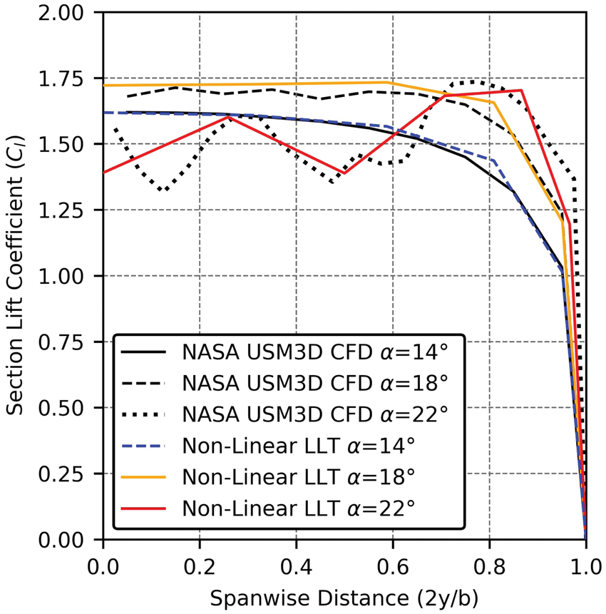
Finally, a neural network model is built by using the parameters as summarized in Table 10.

Table 10.

Hyperparameters for the NN architecture.

Parameters	Values
Number of hidden layers	6
Neurons in the 1st	512
Neurons in the 2nd	256
Neurons in the 3rd	128
Neurons in the 4th	64
Neurons in the 5th	32
Neurons in the 6th	16
Activation function	ReLU
Optimizer	Adam
Initializer	HE normal
Loss function	MAE
Batch size	512
Epoch number	250

In the next step, the model was trained using the network structure and the data sets. The learning curves of the training process are shown in Figure 22. As can be seen from the figures, the loss is converged to the minimum value after 250 epochs. The behavior of the curves and error rate values shows that the learning processes are completed successfully without over- or underfitting.

Figure 22.

Learning curves of developed model. (a) Predicted lift coefficients vs. real values. (b) Predicted drag coefficients vs. real values. (c) Predicted pitching moment coefficients vs. real values.

Furthermore, the error values from the training phase are shown in Table 11. These values were found satisfactory, and the training phase was completed.

Table 11.

Training and validation error values.

Data set	Mean absolute error	Mean squared error
Training	0.00116	0.000018
Validation	0.00124	0.000024

After finishing the training phase, the proposed model is verified with a test set that was not used in the training. The predicted results and real values of the model for the different configurations in the test set are compared in Figure 23. Because there are more than 141,000 test data items, comparisons were visualized by taking 500 points randomly from the data set. As can be seen from the figures, a large number of different target values are distributed over a wide range. However, the model was able to capture even the most extreme values.

Figure 23.

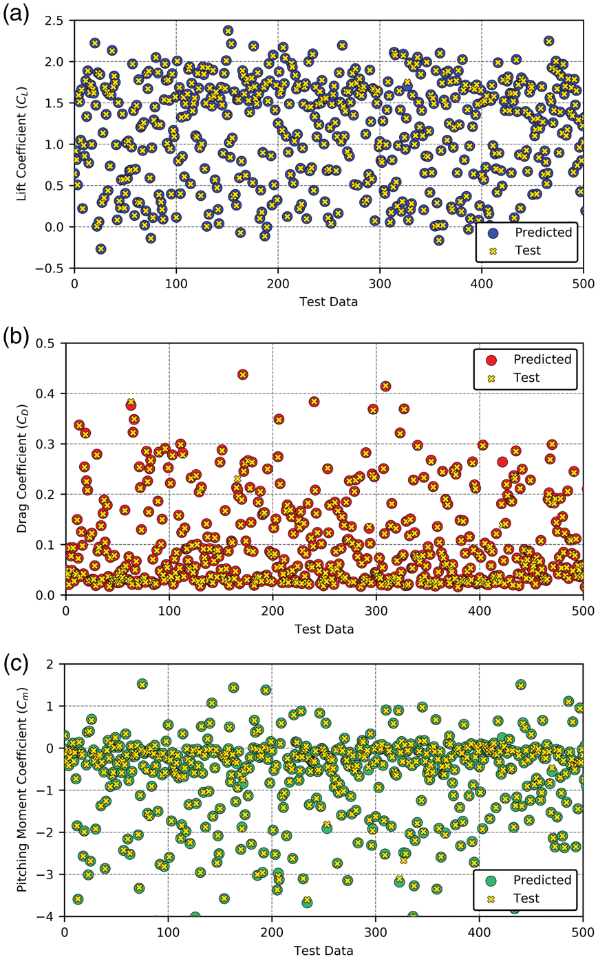
Test set performance on target coefficients.

It must be noted that pitching moment calculations are completed using CG as the reference point at 75% of the chord for all configurations.

To monitor the success of the entire test set of the model, the value of the coefficient of determination, R², is calculated. The results are visualized in Figure 24. In these figures, the x-axis and y-axis represent the real and predicted values, respectively. The value of R² was quite close to 1 in all target coefficients. This situation can also be observed in the figures: almost all the 141,000 test data items are on the regression curve. The total number of values that are not included in the regression line is low enough to be underestimated.

Figure 24.

Test set ( $\approx 141, 000$ data) performance for target parameters.

It is important to note that our proposed method achieves much higher ( $R^{2} = 0.99805 - 0.99976$ ) in comparison to different approaches^40–45 with the coefficient of determination within ( $R^{2} = 0.805 - 0.945$ ) range. This demonstrates the precision and extensive learning capabilities of our proposed approach even in the high angle of attack regimes where fully nonlinear behavior is observed. In the next subsection we will provide these capabilities on various applications.

Application of the surrogate model

In this subsection, the outcomes of several test examples of the current surrogate model are presented to show its generalization capability. As previously explained, the model predicts the nonlinear performance coefficients of the UAV configuration using only geometry data as input (see Figure 1). This gives the model a practicality and computation speed that has never been achieved in any aerodynamic analysis tool that relies on actual computation of the flow dynamics.

In Test Cases A and B, a conventional and a tandem configuration of UAVs with wing profiles used in training the model were chosen as examples. Specifications for UAV geometries are summarized in Table 12.

Table 12.

Specifications for Test Cases A and B.

	Test Case A			Test Case B
Parameters	Wing	Tail	Fuselage	Wing	Tail	Fuselage
Span	2.25	0.9	–	6	3	–
Chord	0.2	0.2	–	0.4	0.4	–
Incidence	0	0	–	1	0	–
Airfoil	2412	0012	–	4412	0012	–
Diameter	–	–	0.2	–	–	0.4
Length	–	–	2	–	–	5
Reynolds	0.4 M	0.4 M	–	0.8 M	0.8 M	–
Location	[0,0,0]	[1,0,0]	[−1,0,0]	[0,0,0]	[2.5,0,0]	[−2.5,0,0]

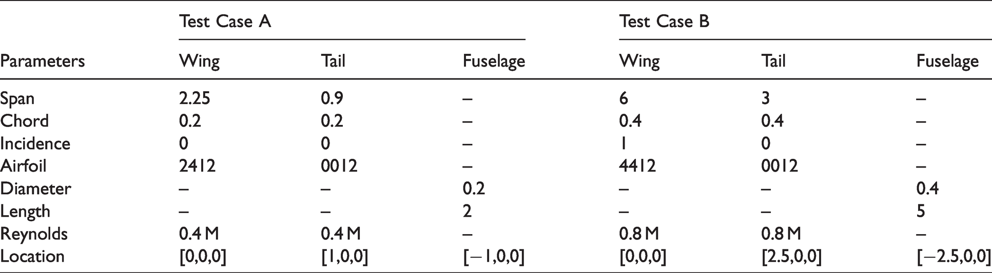
As can be seen from Figure 25, the predicted results are nearly equal to the real values. The neural network model has accurately calculated the lift coefficient in both the linear and nonlinear regions including post-stall for conventional and tandem configurations. Similarly, it has calculated the drag and pitching moment coefficients successfully. Moreover, the model was able to capture pitching moment changes at a high angle of attack due to the nonlinear behavior of the lifting surfaces.

Figure 25.

Test Cases A (conventional) and B (tandem) aerodynamic performance coefficients.

In Test Cases C and D, the same geometries were tested as in the previous example, excluding the wing profiles. This time 3412 and 5412 were used as wing profiles to test the model generalization capability. The camber ratio of these generic profiles differs from those used in training the model. However, as described in the previous sections, the camber ratio of the profile is given as input to the model. Thus, the developed model is intended to calculate other profiles in the NACA 4-series. The profiles used in the test studies are summarized in Table 13.

Table 13.

NACA series airfoils used in test cases.

	Conventional		Tandem
Surface	Case A	Case C	Case B	Case D
Wing	2412	3412	4412	5412
Tail	0012	0012	0012	0012

The results of these analyses are presented in Figure 26. As the results show, the new developed neural network model is compatible with the real values in both the linear and nonlinear regions. In this sense, it can be clearly stated that the proposed model can calculate nonlinear effects on the lift curves even in the post-stall regime. The success rates in the drag and pitching moment coefficients are also very high. The predicted results are almost 1-1 compatible with the real results. Again, it should be noted that these profiles were not used in model training. However, the artificial neural network was able to calculate the impact on aerodynamic performance owing to its ability to interpolate between profiles. Dozens of applications made in addition to these test studies show that the model can calculate interval design points with very accurately by covering the design space.

Figure 26.

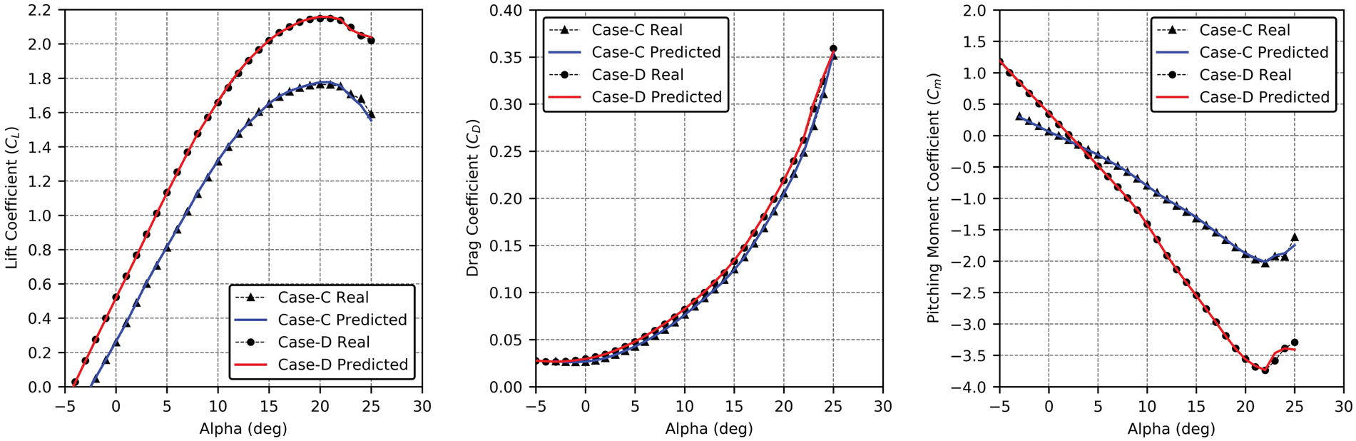
Test Case C (conventional) and D (tandem) aerodynamic performance coefficients.

To demonstrate the feasibility of the methodology, developed surrogate model was used as the aerodynamic solver for an optimization study of small UAVs. For this purpose, the model was transferred to Matlab as a function. A simple design optimization study was generated using the genetic algorithm toolbox.

In the GA approach, an initial set of designs is generated using design variables remaining within predetermined limits. For each design, fitness values are calculated using the cost function, and a random subset is selected from the current design set for those that are better fits. Random operations are used to create new designs using the subset of selected designs. In this methodology, while the gene represents the design variable, the chromosome is used to name the design point. Aerodynamic characterization of new individuals obtained after crossovers and mutations can be provided instantly by the currently developed AI model, and fitness values can be calculated.

By using the Case-A configuration in the previous test studies, an attempt was made to maximize the endurance performance of this vehicle. To achieve this objective, the wing profile and incidence angles of the lifting surfaces have been optimized in a way that will ensure static stability conditions and prevent the maximum drag limit from being exceed. The purpose of this optimization problem is to obtain a configuration with maximum efficiency that provides the required stability and aerodynamic conditions. The optimization problem can be defined as

\underset{x}{maximize} f (x) = \frac{L}{D}

(43)

subject to 0.35 < C_{L} < 0.45

(44)

C_{m_{0}} > 0

(45)

C_{m_{α}} < 0

(46)

C_{D} < 0.035

(47)

where x includes the cruise angle of attack, wing airfoil camber ratio, and wing and tail incidence angles. The first inequality constraint is related to the lift coefficient, and this is necessary to balance the weight without changing the cruise speed dramatically. The minimum value of

C_{m_{0}}

is determined as zero, because it is one of the major constraints of longitudinal static stability. Moreover, the stick fixed pitching moment slope must be negative for stable longitudinal flight. As a final condition of inequality, the total drag coefficient is limited to that in the basic configuration to ensure equality of the thrust and drag forces.

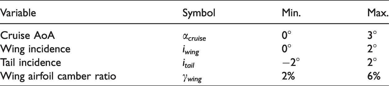
In this optimization problem, geometry variables are limited to the cruise angle of attack, the wing section camber ratio, and the incidence angles of the lifting surfaces (see Table 14). The aim is to increase the aerodynamic efficiency with small profile changes while preserving the main geometry dimensions. However, it is possible to use all the other 14 parameters related to the wing, tail, and fuselage components shown in Table 7.

Table 14.

Variables with lower and upper bounds.

Variable	Symbol	Min.	Max.
Cruise AoA	α_cruise	$0 °$	$3 °$
Wing incidence	i_wing	$0 °$	$2 °$
Tail incidence	i_tail	$- 2 °$	$2 °$
Wing airfoil camber ratio	γ_wing	2%	6%

The speed of the surrogate model ensured that the optimization study, which included hundreds of iterations, was completed in 2–3 s. The new values of the variables are shown in Table 15.

Table 15.

Optimized geometry variables.

Configuration	γ_wing	i_wing	i_tail
Test Case A	2.00%	$0.00 °$	$0.00 °$
Optimized	2.86%	$0.57 °$	$0.04 °$

In addition, the new wing profile that the program optimally designed in the NACA 4-series airfoil family and the previous airfoil are compared in Figure 27. This example directly emphasizes the design flexibility of the method.

Figure 27.

NACA 2412 and the new optimized airfoil geometry.

According to the results of this study, the aerodynamic efficiency increased by 5.18%. Several different geometry parameters such as the wing, tail, and fuselage dimensions can easily be used as variables in similar optimization studies. The examples show that this developed model can be an essential aerodynamic solver for large-scale aircraft design optimization studies.

Conclusions

This article presents a new computational aerodynamic method and its surrogate model to predict the nonlinear aerodynamic performance of small UAVs. The developed nonlinear lifting line tool can calculate the performance of UAV configurations in a remarkably efficient way in terms of processing time and power. In the analyses, it was observed that the method can solve 90 different UAV configurations at 30 different angles of attack in 1 s running time. When the computational complexity of the developed tool was examined, it was found that it has a linear time, O(n), behavior. However, because the method is based on Prandtl’s lifting line theory, it needs 2D performance inputs of the section profiles of the lifting surfaces. To eliminate this deficiency, a new deep learning-based model is trained using data of 94,500 UAV configurations produced by the aerodynamic method. Because of the complex artificial neural networks supported by the new feature sets, the model has a mean absolute error order of $1 \times 10^{- 3}$ . The developed neural network model provides a stand-alone analysis tool and the basis for bidirectional design optimization for small UAVs. In addition to this, the model offers a starting point for an inverse tool that can calculate geometry parameters including wing or tail dimensions, section profiles, incidence angles, and angles of attack of configurations for a given design condition. At the end of the article, a simple genetic algorithm-based optimization application was conducted, and the aerodynamic efficiency of a generic UAV configuration was increased by 5.18% in a few seconds. Thus, the developed model provides a highly capable aerodynamic solver for such design optimization studies.

However, the proposed approach also has some limitations. Because the method is based on classical lifting line theory, it is not suitable for unconventional geometries that have wings with high sweep or dihedral angles and low aspect ratios. Elimination of this deficiency is possible with the development of a new nonlinear tool based on the panel methods. In addition, in this study, the training of the AI model was provided by using the mathematical formulation of the NACA-4 series airfoil family. To improve the validity of the surrogate model, the training data need to be further enhanced to cover different airfoil families.

Our current research is focused on extending the proposed methodology to capture a wider design space including further effects on the performance coefficients.

Supplemental Material

sj-pdf-1-mav-10.1177_17568293211016817 - Supplemental material for A new nonlinear lifting line method for aerodynamic analysis and deep learning modeling of small unmanned aerial vehicles

Supplemental material, sj-pdf-1-mav-10.1177_17568293211016817 for A new nonlinear lifting line method for aerodynamic analysis and deep learning modeling of small unmanned aerial vehicles by Hasan Karali, Gokhan Inalhan, M Umut Demirezen and M Adil Yukselen in International Journal of Micro Air Vehicles

Footnotes

Declaration of conflicting interests

The author(s) declared no potential conflicts of interest with respect to the research, authorship, and/or publication of this article.

Funding

The author(s) received no financial support for the research, authorship, and/or publication of this article.

ORCID iDs

Hasan Karali

Gokhan Inalhan

References

NATO Standardization Agency (NSA). Guidance for the training of unmanned aircraft systems (UAS) operators. Nato Standard ATP-3.3.7, NATO/OTAN, 2014.

Mueller

On the birth of micro air vehicles. Int J Micro Air Veh 2009; 1: 1–12.

Ure

Inalhan

Autonomous control of unmanned combat air vehicles: design of a multimodal control and flight planning framework for agile maneuvering. IEEE Control Syst Mag 2012; 32(5): 74–95.

Kody

Bramesfeld

Small UAV design using an integrated design tool. Int J Micro Air Veh 2012; 4: 151–164.

Karali

Demirezen

Yukselen

, et al. Design of a deep learning based nonlinear aerodynamic surrogate model for UAVs. In: AIAA Scitech 2020 forum, January 2020, Orlando, FL, p.1288. https://doi.org/10.2514/6.2020-1288

ARC UAV Flight Test Video, https://www.youtube.com/watch?v=Cy_ZwTixUuI (2018, accessed 15 December 2020).

Karali

Yukselen

Inalhan

A new non-linear lifting line method for 3D analysis of wing/configuration aerodynamic characteristics with application to UAVs. In: AIAA Scitech 2019 forum, January 2019, San Diego, CA, p.2119, https://doi.org/10.2514/6.2019-2119

Prandtl

Tragflügeltheorie. i. mitteilung.

Nachrichten von der Gesellschaft der Wissenschaften zu Göttingen, Mathematisch-Physikalische Klasse 1918; 1918: 451–477.

Prandtl

Applications of modern hydrodynamics to aeronautics. NACA technical report 116, National Advisory Committee for Aeronautics, 1923.

10.

Tani

A simple method of calculating the induced velocity of a monoplane wing. Report of the Aeronautical Research Institute, Tokyo Imperial University, Japan, 1934.

11.

Sivells

Neely

RH.

Method for calculating wing characteristics by lifting-line theory using nonlinear section life data 865. National Advisory Committee for Aeronautics, 1947.

12.

Weissinger

The lift distribution of swept-back wings [Uber die Auftriebsverteilung von Pfeilflugeln]. NACA technical report 1120, National Advisory Committee for Aeronautics, USA, 1947, https://ntrs.nasa.gov/search.jsp?R=20030064148

13.

Phillips

Snyder

DO.

Modern adaptation of Prandtl’s classic lifting-line theory. J Aircraft 2000; 37: 662–670.

14.

Piszkin

Levinsky

Nonlinear lifting line theory for predicting stalling instabilities on wings of moderate aspect ratio. Defense Technical Information Center, 1976.

15.

de Vargas

LAT

de Oliveira

PHIA.

A fast aerodynamic procedure for a complete aircraft design using the know airfoil characteristics. SAE technical paper, 2006. https://doi.org/10.4271/2006-01-2818

16.

Falkner

VM.

The calculation of aerodynamic loading on surfaces of any shape. Technical report, Aeronautical Research Council London, UK, 1943.

17.

Mukherjee

Gopalarathnam

Poststall prediction of multiple-lifting-surface configurations using a decambering approach. J Aircraft 2006; 43: 660–668.

18.

Sugar Gabor

Koreanschi

Botez

A new non-linear vortex lattice method: applications to wing aerodynamic optimizations. Chin J Aeronaut 2016; 29: 1178–1195.

19.

Deperrois

Xflr5 analysis of foils and wings operating at low Reynolds numbers. Guidelines for XFLR5, 2009.

20.

Kinney

McDonald

VSPAero/OpenVSP integration, 2015.

21.

Melin T.

Tornado, a vortex lattice MATLAB implementation for linear aerodynamic wing applications. Master’s Thesis, KTH, Sweden, 2013.

22.

Melin

Tornado: a vortex lattice method implemented in Matlab. Glenn Research Center, NASA, 2017

23.

Hunsaker

A numerical lifting-line method using horseshoe vortex sheets. In: Rocky Mountain Space Grant Consortium Meeting Proceedings, 2001, Logan, UT.

24.

Karali

Yukselen

MA.

Nonlinear analysis of 3D wing aerodynamic characteristics (in Turkish). In: VII. Ulusal Havacilik ve Uzay Konferansi, September 2018, Samsun, Turkey, http://www.uhuk.org.tr/bildiri.php?No=UHUK-2018-080

25.

Rasmussen

Smith

DE.

Lifting-line theory for arbitrarily shaped wings. J Aircraft 1999; 36: 340–348.

26.

Phillips

WF.

Lifting-line analysis for twisted wings and washout-optimized wings. J Aircraft 2004; 41: 128–136.

27.

Wickenheiser

Garcia

Aerodynamic modeling of morphing wings using an extended lifting-line analysis. J Aircraft 2007; 44: 10–16.

28.

Ostler

Bowman

Snyder

, et al. Performance flight testing of small, electric powered unmanned aerial vehicles. Int J Micro Air Veh 2009; 1: 155–171.

29.

Anderson

Jr Corda

Van Wie

DM.

Numerical lifting line theory applied to drooped leading-edge wings below and above stall. J Aircraft 1980; 17: 898–904.

30.

Bronz

Moschetta

Brisset

, et al. Towards a long endurance MAV. Int J Micro Air Veh 2009; 1: 241–254. DOI: 10.1260/175682909790291483

31.

Bronz

Hattenberger

Moschetta

JM.

Development of a long endurance mini-UAV: eternity. Int J Micro Air Veh 2013; 5: 261–272.

32.

Ben Mosbah

Botez

Dao

TM.

A hybrid original approach for prediction of the aerodynamic coefficients of an atr-42 scaled wing model. Chin J Aeronaut 2016; 29: 41–52.

33.

Zelong

Wang

Qiu

, et al. Aerodynamic coefficient prediction of airfoils with convolutional neural network, In: Zhang X. (eds) The Proceedings of the 2018 Asia-Pacific International Symposium on Aerospace Technology (APISAT 2018), 2018, pp.34–46, https://doi.org/10.1007/978-981-13-3305-7_3

34.

Chen

Qian

, et al. Multiple aerodynamic coefficient prediction of airfoils using a convolutional neural network. Symmetry 2020; 12: 544.

35.

Rajkumar

Bardina

Training data requirement for a neural network to predict aerodynamic coefficients. In: AeroSense 2003: SPIE’s 17th annual international symposium on aerospace/defense sensing, April 2003, Orlando, FL, https://doi.org/10.1117/12.486343

36.

Secco

Mattos

Artificial neural networks to predict aerodynamic coefficients of transport airplanes. Aircraft Eng Aerosp Technol 2017; 89: 211–230.

37.

Wang

Qian

Unsteady aerodynamic modeling at high angles of attack using support vector machines. Chin J Aeronaut 2015; 28: 659–668.

38.

Gomec

Canibek

Aerodynamic database improvement of aircraft based on neural networks and genetic algorithms. In: 7th European conference for aeronautics and space sciences, July 2017, Milan, Italy, https://doi.org/10.13009/EUCASS2017-226

39.

Wallach

Mattos

Girardi

, et al. Aerodynamic coefficient prediction of transport aircraft using neural network, 2012. https://arc.aiaa.org/doi/abs/10.2514/6.2006-658

40.

Sharma

Singh

, et al. Aerodynamic modeling of attas aircraft using Mamdani fuzzy inference network. IEEE Trans Aerosp Electron Syst 2020; 56: 3566–3576., DOI: 10.1109/TAES.2020.2975447

41.

Sharma

Singh

Verma

NK.

Data driven aerodynamic modeling using mamdani fuzzy inference systems. In: 2018 International conference on sensing, diagnostics, prognostics, and control (SDPC), 2018, pp.359–364, https://doi.org/10.1109/SDPC.2018.8664870

42.

Jang

JR.

Anfis: adaptive-network-based fuzzy inference system. IEEE Trans Syst Man Cybern 1993; 23: 665–685.

43.

Takagi

Sugeno

Fuzzy identification of systems and its applications to modeling and control. IEEE Trans Syst Man Cybern 1985; SMC-15: 116–132.

44.

Raisinghani

Ghosh

Kalra

PK.

Two new techniques for aircraft parameter estimation using neural networks. Aeronaut J (1968) 1998; 102: 25–30.

45.

Sanwale

Singh

DJ.

Aerodynamic parameters estimation using radial basis function neural partial differentiation method. Def Sci J 2018; 68: 241–250.

46.

Cummings

Mason

Morton

, et al. Applied computational aerodynamics: a modern engineering approach. Cambridge Aerospace Series. Cambridge: Cambridge University Press, 2015.

47.

Abbott

Von Doenhoff

Stivers

Jr.

Summary of airfoil data. Naca technical report 824, National Advisory Committee for Aeronautics, USA, 1945, https://ntrs.nasa.gov/search.jsp?R=19930090976

48.

Anderson

Jr.

Fundamentals of aerodynamics. Boston, MA: McGraw-Hill Education, 2010.

49.

Katz

Plotkin

Low-speed aerodynamics. 2nd ed. Cambridge Aerospace Series. Cambridge: Cambridge University Press, 2001.

50.

Ostowari

Naik

Post-stall wind tunnel data for NACA 44XX series airfoil sections. Technical report, Texas A&M University, USA, 1985.

51.

McLain

DJ.

A U.S. Navy RQ-2B pioneer unmanned aerial vehicle. Official Website of the United States Navy, 2005, https://www.navy.mil/view_image.asp?id=25689

52.

Tetreau

RA.

A U.S. Marine Corps RQ-7B shadow unmanned aerial vehicle. Official Website of the United States Navy, 2011, https://www.navy.mil/view_image.asp?id=100815

53.

Petrilli

Paul

Gopalarathnam

, et al. A CFD database for airfoils and wings at post-stall angles of attack. In: 31st AIAA applied aerodynamics conference, June 2013, p.2916, https://doi.org/10.2514/6.2013-2916

54.

Phillips

Anderson

Jenkins

, et al. Estimating the low-speed downwash angle on an aft tail. J Aircraft 2002; 39: 600–608.

55.

Sadraey

MH.

Aircraft design: a systems engineering approach. Aerospace Series. Chichester: John Wiley and Sons, 2013.

56.

Roskam

Lan

CTE.

Airplane aerodynamics and performance. Lawrence, KS: DARcorporation, 1997.

57.

Nelson

. Flight stability and automatic control. vol. 2. New York, NY: WCB/McGraw Hill, 1998.

58.

Yuksek

Vuruskan

Özdemir

, et al. Transition flight modeling of a fixed-wing VTOL UAV. J Intell Rob Syst 2016; 84: 83–105.

59.

Yuksek

Ure

Caliskan

, et al. Fault tolerant heading control system design for Turac unmanned aerial vehicle. Trans Inst Meas Control 2017; 39: 267–276.

60.

Uzun

Modelling and flight control system design of micro UAV. Undergraduate Thesis, Istanbul Technical University, Turkey, 2018.

61.

Finck

RD.

USAF (United States Air Force) stability and control DATCOM (Data Compendium). Final report AFWAL-TR-83-3048, McDonnell Douglas Corporation Douglas Aircraft Division, USA, 1978.

62.

Drela

Xfoil: an analysis and design system for low Reynolds number airfoils. In: Low Reynolds number aerodynamics. New York, NY: Springer, 1989, pp.1–12.

63.

Horn

Pack

Rieger

The autofeat python library for automated feature engineering and selection. preprint arXiv:190107329 2019, https://arxiv.org/abs/1901.07329

64.

Nair

Hinton

GE.

Rectified linear units improve restricted Boltzmann machines. In: Proceedings of the 27th international conference on machine learning, ICML’10, Madison, WI: Omnipress. pp.807–814. https://dl.acm.org/doi/10.5555/3104322.3104425

65.

Zhang

Ren

, et al. Delving deep into rectifiers: surpassing human-level performance on imagenet classification. CoRR, 2015, https://arxiv.org/abs/1502.01852

66.

Kingma

Adam: a method for stochastic optimization. In: 3rd International conference for learning representations, San Diego, CA, May 2015, https://arxiv.org/abs/1412.6980

Supplementary Material

Please find the following supplemental material available below.

For Open Access articles published under a Creative Commons License, all supplemental material carries the same license as the article it is associated with.

For non-Open Access articles published, all supplemental material carries a non-exclusive license, and permission requests for re-use of supplemental material or any part of supplemental material shall be sent directly to the copyright owner as specified in the copyright notice associated with the article.

0.00 MB

0.22 MB