Vortex filamentation and fragmentation phenomena in flapping motion and effect of aspect ratio and frequency on global strain,rotation,and enstrophy

Abstract

In the present study, flow field around rigid flat plate wings executing main flapping motion has been studied using phase-locked two-dimensional particle image velocimetry measurements. Experiments have been conducted in water as a fluid medium for an asymmetric upper–lower stroke single degree of freedom main flapping motion. Two different aspect ratio (1.5 and 1.0) rectangular wings at 1.5 and 2.0 Hz flapping frequency in hovering flight mode (advance ratio, J = 0), zero wing pitch angle, and chord-based Reynolds number of the order of 10⁴ have been studied. Velocity field and vorticity field with λ₂ criterion information have been obtained for the complete stroke in great detail to reveal the minute aspects of flow dynamics. The flow features during the downstroke and upstroke have been observed to be consistent for all four cases investigated. The predominant characteristic of the flow during downstroke and upstroke has been referred to as vortex filamentation and fragmentation phenomena. Quantities such as circulation, rate of strain, rate of rotation, and enstrophy have been studied to identity the effect of minor change in aspect ratio and flapping frequency. It is found that for higher aspect ratio wing hyperbolic behavior is predominant except for end of downstroke and beginning of upstroke where elliptic behavior is observed. For lower aspect ratio, wing elliptic behavior is predominant except for end of upstroke and beginning of downstroke where hyperbolic behavior is seen. The hyperbolic behavior became stronger at higher frequency. From enstrophy distribution it is evident that higher frequencies play a more dominant role than aspect ratio in determining the budget.

Introduction

Natural flyers have always been fascinating and inspiring for humans. To understand and mimic them is a significant challenge. Physical and numerical experiments with different analysis tools are necessary to make a headway. The studies reported by Weis-Fogh, ¹ Lighthill, ² Dickinson and Götz, ³ Wootton, ⁴ Dickinson, ⁵ Ellington et al., ⁶ Ellington, ⁷ Dickinson et al., ⁸ and Sun and Tang ⁹ were immense in contribution and laid a path to understand flapping flight. Hong and Altman,^10,11 Jardin et al., ¹² Massey et al., ¹³ Krashanitsa et al., ¹⁴ Mazaheri and Ebrahimi,^15–17 Suryadi et al., ¹⁸ Jones and Babinsky, ¹⁹ Lua et al., ²⁰ Ozen and Rockwell, ²¹ Curtis et al., ²² Granlund et al., ²³ Goli et al., ²⁴ and Lua et al. ²⁵ report various studies performed on flapping wings with an intention to visualize and understand the flow field behavior of heaving, pitching, and combined heaving–pitching of rigid airfoils, flat plates, and wings of low aspect ratio (AR).

Micro air vehicles (MAVs) are based on fixed wing, rotary wing, or flapping wing configurations. Similar configurations are possible in water-based applications which may be called micro under water vehicles (MUWVs). For development of such miniature vehicles for either airborne or water-based application, one of the key parameters is the selection of kinematics. Simplicity in design of kinematics is always recommendable. Choice of kinematics depends on desired application of the MAV. With regards to flapping wing MAV, single degree of freedom flapping kinematics has been used by Mazaheri and Ebrahimi^15–17 and Hu et al. ²⁶ for different frequencies, AR, materials, and they have discussed especially on force measurements and have reported that higher flapping frequencies and high AR would lead to higher force/moments. It has also been stated that rigid wing would lead to higher forces in comparison with flexible wings while flexible wings would have higher wing efficiency. Hong and Altman^10,11 have used similar kinematics as abovementioned literature and have concentrated on force measurements. Some of the results cover velocity and vorticity distribution and it was stated that spanwise flow plays an important role in determining the force generation. Ozen and Rockwell ²¹ have studied the flow field for a rigid wing with freestream velocity. Goli et al. ²⁴ have compared the flow field for rigid and flexible wings at 1 Hz flapping frequency in a quiescent fluid to capture the flow field along the wing span.

Natural flyers like hoverflies, dragonflies, and bumblebees create asymmetry in flapping during their flight in hover or forward flight for better lift/normal force generation.^27–30 Similar results were confirmed through two-dimensional numerical studies reported by Zhu and Zhou, ²⁹ Wang et al., ³⁰ Sarkar and Venkatraman, ³¹ and Sarkar et al. ³² These works indicate that greater normal/lift force can be generated if the downstroke is faster than upstroke. Experimental kinematics of Hong and Altman^10,11 resulted in faster downstroke. However, the authors have not emphasized on determining its effect on flow field and it is not apparent whether it would generate higher forces or not.

For an MAV, necessary forces and moments have to be generated in order to make it fly and fulfill its mission objectives. Flow field around the wing would be primarily responsible for generating them. So it would always be important to study different aspects of the flow field like velocity, vorticity, circulation, rate of strain, rate of rotation, etc. and to find the correlation between these aspects and the forces. These correlations would help to develop more optimized or efficient MAVs in future. So the present study has concentrated on a detailed flow field analysis but not on direct force measurement.

During the course of wing flapping, turbulence is generated both due to the shear produced at the wing surface and the body forces produced due to its movement. The turbulent flow field is characterized by a rich distribution of vorticity. The vorticity field gets intensified through a process of stretching or attenuated by a process of compression. The vorticity field advects in a chaotic manner straining the vortex tubes and sheets into finer structures which is referred to as vortex stretching. The circulation is closely connected with the vorticity distribution in a flow field. Under certain underlying assumptions, material derivative of circulation is found to be invariant as per the Kelvin’s circulation theorem. Due to wing flapping, the flow field undergoes displacement, strain, and rotation. These effects are studied through the velocity, rate of strain tensor, and rate of rotation tensor in order to acquire a deeper understanding of the effect of the flapping wing on the flow field and vice versa in a reciprocal manner. The energy contained in the vorticity generated by wing motion is concentrated in the integral scale large eddies while enstrophy and therefore dissipation is mostly confined to the microscale small eddies. Enstrophy is depleted at the microscales due to viscous effects. ³³ The enstrophy evolution involves interplay between rate of strain, rate of rotation, and viscous dissipation. These interactions are very complex, often three-dimensional and not revealed directly by either velocity or vorticity fields. Within the limitation of two-dimensional flow field data enstrophy evolution has been studied in the present problem to obtain some trends of its variation related to frequency and AR changes of the flapping wing. This study is relevant because it helps identify regimes in which rate of strain and rate of rotation interact favorably leading to enstrophy generation which indicates formation of intense vorticity pockets. Such pockets before getting dissipated are expected to influence and often augment the performance of the flapping wing through effective wake capture, upwash–downwash effects, etc. Dong et al. ³⁴ have studied two jet-like structures which significantly contribute to lift generation of a flapping wing in hovering motion and found that they are regions of high enstrophy. This is an example of an enhanced enstrophy region affecting performance of a flapping wing.

The present study focuses on velocity field and vorticity field with λ₂ criterion information for the complete stroke in great detail to reveal the minute aspects of flow dynamics. A common phenomenon has been observed during the flapping cycle irrespective of change in flapping frequency and AR (for four different cases) studied in the present work which has been referred as vortex filamentation and fragmentation. Mazaheri and Ebrahimi^15–17 and Hu et al. ²⁶ studied one degree of freedom flapping kinematics as in the present case. However, they emphasized on force measurements while the present study focuses on varied aspects of the flow field. Ozen and Rockwell ²¹ studied one degree of freedom flapping kinematics with angular symmetry under the effect of freestream velocity. They reported the study on one particular AR and one particular flapping frequency which are different from the present study. The present study is carried out with angular asymmetry keeping in mind that it would be useful for force generation. The motivation behind using the asymmetry in flapping is based on natural flyers and the abovementioned literature on two-dimensional numerical studies. The entire downstroke and upstroke flow fields were studied to extract details of the flow features which were not identical due to angular asymmetry. Ozen and Rockwell ²¹ studied half of the complete stroke because of angular symmetry. The present investigation included two different ARs (1.0 and 1.5) and two different flapping frequencies (1.5 and 2.0 Hz) without any freestream effect. Quantities such as circulation, rate of strain, rate of rotation, and enstrophy have been studied and the effect of minor change in AR and flapping frequency on such quantities has been identified. This flow field-based analysis has not been so extensively reported for the kinematics used in the present work and most of the other similar kinematics to the best of the authors’ knowledge. The present study is significant because flow features were visualized at discrete phase wise flapping wing orientations and effect of AR and frequency was investigated by using different analysis tools.

Materials and methods

Flapping mechanism and water tank

The main flapping mechanism design is similar to that reported in Mazaheri and Ebrahimi^15–17 (patent lies with Kim et al., ³⁵ “Cybrid P1 remotely controlled ornithopter”) and dimensions were reported in Goli et al. ²⁴ The main flapping motion is a single degree of freedom motion in which the wing undergoes pure flapping with a pivot/hinge point located at a fixed distance from the wing root. Further, the wing chordwise pitch is maintained as zero degree and the wing has zero deviation from stroke plane while it is executing the flapping motion. The four-bar mechanism as shown in Figure 1, in which the DC motor is connected to the pinion, transforms the rotational motion to desired main flapping motion. The driving motor is powered directly by a stable DC power supply, by which the flapping frequency is controlled by altering the input voltage. Its dimensions are chosen so that 1:3 ratio lower half stroke to upper half stroke asymmetry one degree of freedom flapping motion is achieved.

Figure 1.

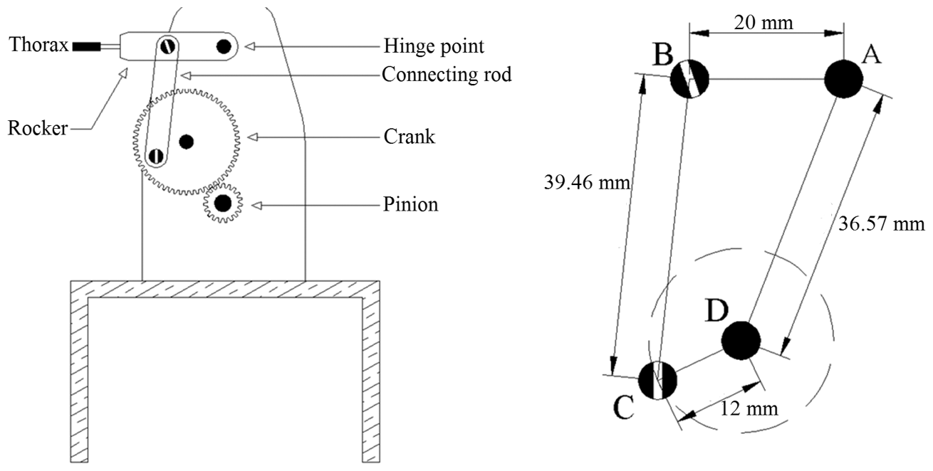
(a) Schematic of main flapping mechanism and (b) crank–rocker four-bar mechanical linkage. ²⁴

The experiments have been carried out in a water tank with dimensions of 0.9 m × 0.6 m × 0.79 m. Schematic of complete setup is shown in Figure 2. The dimensions of the rectangular planform flapping wings are shown in Table 1. The wings are made of Perspex and they have 1.5 mm thickness. In the present experiments wing deflection has been recorded and found to be negligible. Therefore, they are considered as rigid. The dimensions of thorax are 20 mm length, 10 mm width, and 3 mm thickness. It weighs 2 g.

Figure 2.

Schematic of complete setup used for PIV measurements.

Table 1.

Wing details.

Span, s (mm)	Chord, c (mm)	thickness, t (mm)	AR
60	40	1.5	1.5
40	40	1.5	1.0

AR: aspect ratio.

Procedure

The flapping mechanism is mounted on a test stand and fully immersed in the water tank with free surface of water exposed to the atmosphere. The fluid is initially maintained in quiescent condition. When the wing is flapping in such a medium it is in hover. The primary motivation behind using water was to exploit better quality particle image velocimetry (PIV) imaging with more homogeneous dispersion of seeding particles in water and avoiding the complications involved in handling gappy PIV data. ³⁶ Moreover, the experimental setup for the present work has been designed in such a manner that the flow around the flapping wing and its neighborhood would suffer minimum interference from sidewalls of the water tank in which the experiments have been conducted or from free surface sloshing effects. Hence the flapping mechanism had to be fully immersed deep inside the water tank with the walls and free surfaces at sufficiently large distances so that the near wing flow field would not be perturbed by boundary proximity effects. The incident and reflected perturbations at the side walls and free surface were analyzed over large number of wing flapping cycles using PIV images and were found to be of negligible order.

The water is seeded with hollow glass particles having a mean diameter of 10 µm and density of 1.1 g/cc. The percentage of seeding particles is approximately 10⁻⁵ (40 ml water laden with particles mixed with 426 l of clean water). The experiments have been performed with nominal flapping amplitude of 80° (ϕ_max), with upper half stroke angle (ϕ_a) of 60° and lower half stroke angle (ϕ_b) of 20° from the horizontal line as shown in Figure 3, with zero wing pitch angle and at flapping frequencies of 1.5 and 2 Hz. During the experiments, the actual achieved flapping amplitude (ϕ) with wings attached to the main flapping mechanism is different from nominal flapping amplitude due to inertial loads as shown in Table 2. Downstroke and upstroke are indicated by DS and US, respectively. The flapping amplitude depends on parameters like wing geometry and size, wing material, and operating conditions. Similar observations are reported by Mazaheri and Ebrahimi.^15–17 Power requirements for achieving the desired flapping frequency for a given AR are also shown in Table 2. During the flapping cycle it has been found that the DS is faster than US. Around 39–48% time is spent in the DS depending on the case. Similar observations were made in Hong and Altman^10,11 regarding the fact that DS is faster than US. The PIV measurements have been performed after completing uninterrupted 10 min of wing flapping thus enabling the flow to achieve periodic state of unsteadiness which ensures statistically stationary flow field data. The tests have been conducted by illuminating the flow along the span of the wing, with the laser sheet aligned to the mid chord position of the wing as shown in Figures 4 and 5. Hong and Altman ¹¹ reported that in flapping wing fluid dynamics, spanwise flow plays a significant role in lift generation. At each discrete flapping angle, ϕ, three instantaneous velocity vector fields are obtained and mean of these fields has been calculated to find the phase-locked average velocity vector field. All flow field analysis is based on the average velocity field. The tests have been performed for two different AR wings at two different frequencies and results are shown below in the respective order. Flapping mechanism has been oriented such that laser sheet falls on the designated location of the wing. The achieved flow parameters in the present study are mentioned in Table 3.

Figure 3.

Schematic of main flapping motion.

Table 2.

Achieved flapping amplitude.

	Wing type f (Hz)		ϕa (°)	ϕb (°)	ϕa (°)	ϕb (°)	ϕmax (°)	Power (W)
Case	(AR)		DS	DS	US	US
No wing	No wing	–	60	20	60	20	80
I	1.5	1.5	54.5	13.5	55.5	12.5	69	10.25
II	1.0	1.5	58.5	14.5	59.5	13.5	74	06.01
III	1.5	2.0	54.5	13.5	55.5	12.5	69	19.10
IV	1.0	2.0	58.5	14.5	59.5	13.5	74	08.75

AR: aspect ratio; DS: downstroke; US: upstroke.

Figure 4.

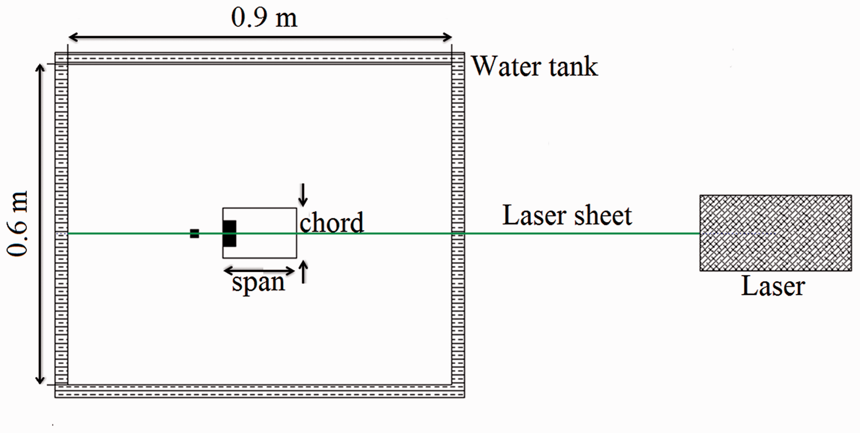
Schematic plan view of PIV setup and wing position (along the spanwise direction, volume of tank 0.9 m × 0.6 m × 0.79 m).

Figure 5.

Schematic front view (dimensions in mm).

Table 3.

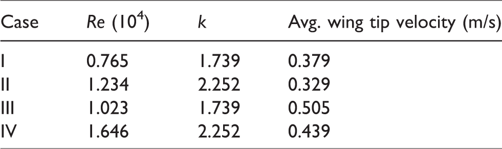
Flow parameters.

Case	Re (104)	k	Avg. wing tip velocity (m/s)
I	0.765	1.739	0.379
II	1.234	2.252	0.329
III	1.023	1.739	0.505
IV	1.646	2.252	0.439

Flow parameters

The relevant nondimensional flow parameters for the present study are discussed briefly in this section as mentioned in Table 3.

Reynolds number is defined as the ratio of inertial forces to viscous forces. Since the present investigation is performed at low–moderate Reynolds number, the viscous forces are comparable to inertial forces and therefore Reynolds number is a very important parameter which influences flow behavior in this flow regime, where ρ is the density of fluid, U_ref is the forward velocity, L is the reference length, μ is the dynamic viscosity of fluid, ϕ_max is the flapping amplitude as shown in Table 2, f is the flapping frequency, b is the span or chord of the wing, AR is the aspect ratio of wing, ν is the kinematic viscosity of fluid (1.004 × 10⁻⁶ m²/s)

$$\mathit{Re}=\frac{\rho U_{\mathit{ref}}\text{L}}{\text{µ}}$$

(1)

In hovering flight, since there is no forward flight velocity, the mean wing tip velocity is considered as U_ref. The Reynolds number for a 3D flapping wing can be written as^7,15

$$\mathit{Re}={\frac{{\varphi }_{\text{max}}fb}{\upsilon }}^2\left(\frac{4}{\text{AR}}\right)$$

(2)

Reduced frequency (k) is a nondimensional parameter defined as a measure of the residence time of a particle convecting over the wing chord compared to the period of motion. It can be interpreted as ratio of flapping frequency to forward velocity

$$k=\frac{2\pi f\text{L}}{2U_{\mathit{ref}}}$$

(3)

In hovering flight, the reduced frequency can be written as

$$k = \frac{\pi }{{\varphi }_{\text{max}}\text{AR}}$$

(4)

Advance ratio (J) is a nondimensional parameter, defined as the ratio of forward flight velocity to wing tip velocity. Advance ratio is used to describe the incoming angle of the fluid relative to the flapping wing

$$J=\frac{U_{\mathit{ref}}}{2\pi f{\varphi }_{\text{max}}}$$

(5)

In hovering flight, since there is no forward flight velocity, J = 0. It is to be noted that in unsteady aerodynamic flows, J < 1 indicates substantial unsteadiness whereas for larger values of J the flow unsteadiness reduces and can be treated as quasi steady.

PIV system and data processing

The PIV system consists of an Nd:YAG dual pulsed laser with maximum energy/pulse of 150 mJ, wave length 1064 nm, laser pulse rate of 14.5 Hz, and 1.5 mm laser thickness. The double shutter CCD camera which is used to acquire the images has 1600 × 1192 pixel resolution at 32 fps. TSI INSIGHT 3G™ software is used to process the captured images by a cross correlation technique with interrogation window size varied, 50% overlapping with a time delay of 400 and 350 µs between two frames for flapping frequency of 1.5 and 2.0 Hz, respectively. The Nyquist method is used for grid generation, where the input images are divided into smaller spots for processing. Gaussian spot masking algorithm is used for conditioning the spots. FFT-based correlation function and Gaussian peak equation are used for correlation mapping and peak identification, respectively. The collected velocity vectors were interpolated into grids of size 3.2 × 3.2 mm² approximately to produce one vector. The output from the processed images yields 12,938 vectors in the view of flow field for 1600 × 1192 pixel resolution. Figure 6 shows a typical example of wing extreme positions, hinge or pivot point, and horizontal line. Pivot point distance is 45 mm from wing root as shown in Figure 5.

Figure 6.

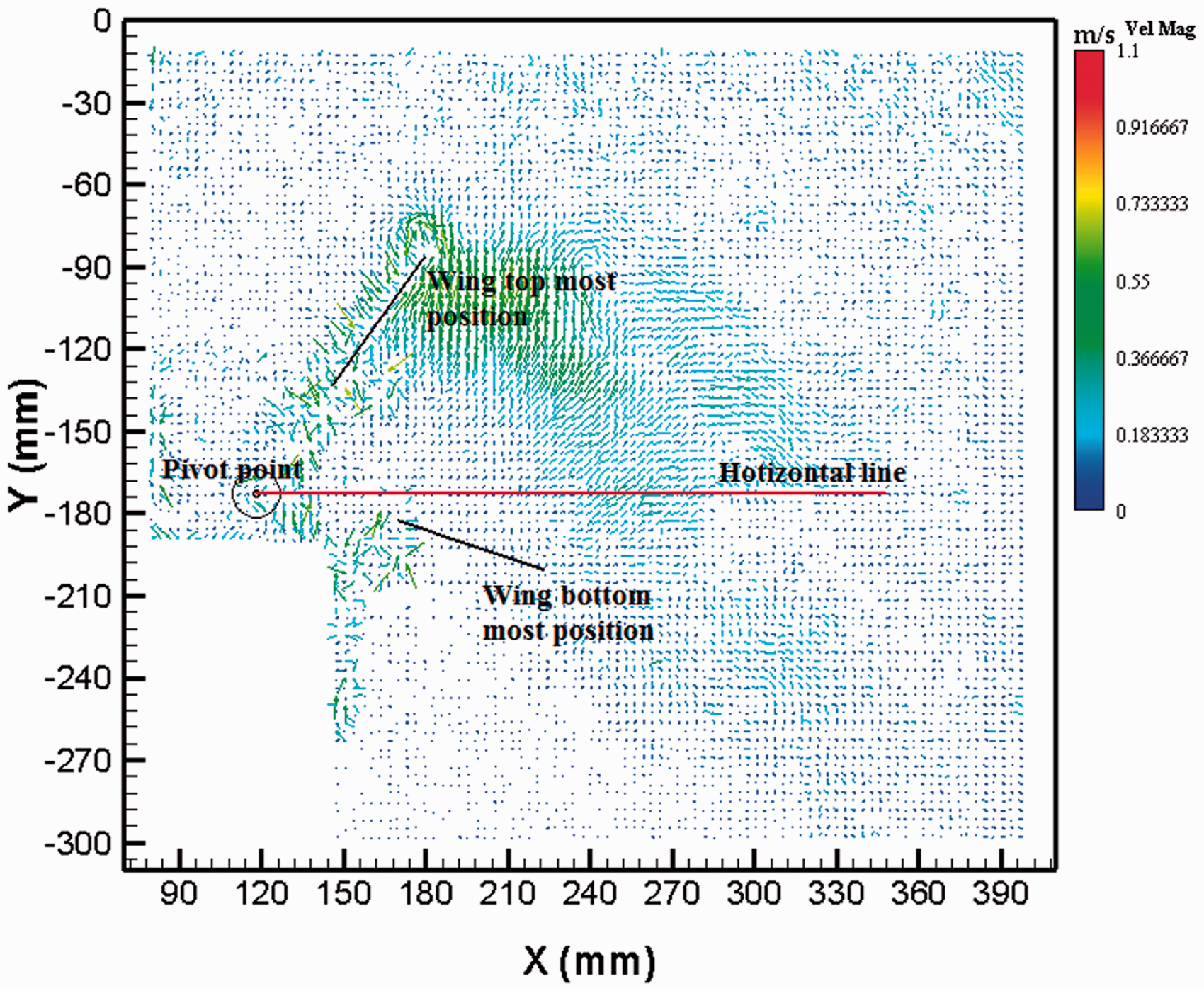
Typical example showing wing extreme positions, pivot point, and horizontal line in a velocity field.

It is known that interrogation window size should be large enough to ensure enough matching particles for robustness and accuracy. However, smaller interrogation windows should be utilized for better spatial resolution in terms of number of vectors. Details in this regard can be found in Wieneke and Pfeiffer ³⁷ and Raffel et al. ³⁸ In the present work, interrogation window size in terms of pixels has been varied from 64 × 64 to 16 × 16 as shown in Figure 7; window overlapping is 50%, displacement range limitation is 25% (N/4) which is called the one-quarter rule.

Figure 7.

Velocity vector field by varying the interrogation window size (velocity magnitude in m/s).

The flow generated by a flapping wing consists of strong shear and vortex-dominated zones in the neighborhood of the wing. By varying the interrogation window size it has been observed that 24 × 24 interrogation window produces reasonably good results and is capable of capturing these features. Therefore, the complete study reported in the following sections is based on 24 × 24 interrogation window.

Certain experimental uncertainties which would affect the accuracy of PIV images are discussed below. The experiments were performed in a water tank with the free surface of water exposed to the atmosphere. Insignificant wave motion was generated at the free surface and negligible effect of the side walls of the tank was recorded through PIV measurements when the flapping mechanism was operated. Thus, boundary effects did not perceivably affect the flow features around the wing. The authors have not shown the complete velocity field in the tank because the velocity values at the virtual boundary of the domain as shown in Figure 6 are very small. It may be worth mentioning that the lateral Perspex walls are located at a distance of 15 times the wing span and the free surface of water is at a distance of 13.16 times the wing span considering the higher AR wing. The ratios would be larger for lower AR wing. The wingtip peak-to-peak displacements are 126.36 and 108.54 mm for higher and lower AR wings, respectively, calculated based on their flapping amplitudes. Similar ratio of peak-to-peak displacement with water tank was reported in Ozen and Rockwell. ²¹

Fabrication error of the wing was maximum 0.25% of the nominal dimension and that of the flapping mechanism to achieve nominal amplitude was ± 0.5° which corresponds to 1.25% error. The magnification factor which is 0.267 mm/pixel would have some effect on the accuracy of PIV image. It is difficult to quantify this uncertainty.

In the PIV images, the laser light reflection from the wing section which affects the intensity in its proximity has been suitably adjusted to the average background intensity using Gaussian Kernel filter.

After processing the data, the spurious vectors were found to be less than 4% from TSI Insight 3G software and local median with 3 × 3 neighborhood size has been used to replace them by interpolation.

Results and discussion

Figures 8 and 9(a) to (e) show the instantaneous velocity vector field and (f) shows the phase-averaged velocity vector field for case I: AR 1.5, f 1.5 Hz and case II: AR 1.0, f 1.5 Hz, respectively, at the beginning of DS. The phase averaging has been carried out by calculating the mean value of U and V component of velocity at each node resulting in a velocity magnitude given by $\sqrt{U_{\mathit{mean}}^2+V_{\mathit{mean}}^2}$ . Phase-averaged velocity field plots have been obtained from instantaneous velocity flow field data using five images when they lie within a range of ± 0.50° and using three images when they lie within ± 0.30° of a specific flap angle. This procedure is repeated for flap angle interval of 1° to cover the entire flapping cycle. The average of five images and three images do not show significant difference in velocity field and coherent structures in flow field. Similar observations were reported by Ozen and Rockwell ²¹ in terms of vorticity. The results shown in further sections of the paper are based on averaging of three images.

Figure 8.

Velocity vector field for case I: AR 1.5, f = 1.5 Hz at the beginning of DS.

Figure 9.

Velocity vector field for case II: AR 1, f = 1.5 Hz at the beginning of DS.

Velocity vector field

In the present section, the velocity vector field for case I: AR 1.5, f = 1.5 Hz has been discussed, and the corresponding flow field is shown in Figures 10 and 11. The flow features exhibit the formation–growth–diffusion of vortices, wake capture, spanwise flow, and their interactions.

Figure 10.

Velocity vector field during DS of flapping cycle for case I: AR 1.5 and f at 1.5 Hz (units in m/s).

Figure 11.

Velocity vector field during US of flapping cycle for case I: AR 1.5 and f at 1.5 Hz (units in m/s).

The flapping angle ϕ in the flapping cycle has been normalized using the following equation (6). The normalized flapping angle ϕ* is represented as a function of instantaneous phase angle and the maximum–minimum phase angle values for the cycle as given below

$${\varphi }^{\text{*}}=\frac{\varphi \left(\text{t}\right)-{\varphi }_{\mathit{beginning}}}{{\varphi }_{\mathit{end}}-{\varphi }_{\mathit{beginning}}}$$

(6)

Using the above equation, the normalized flapping angle varies from 0 to 1 from the beginning to end of each stroke.

Figure 10 shows the velocity field during the DS of the flapping cycle. Starting of the DS is indicated by flap angle ϕ = 54.5° or normalized flapping angle or phase angle ϕ* = 0.0. (Phase angle varies from 0 to 1 from the beginning to end of each stroke.) At this wing orientation we can see a primary vortex at the wing tip rolling up in the inboard direction on the upper surface of the wing. A vertical jet-like flow and a counter rotating vortex at about one span distance to the right of the wing is visible. The beginning of the downward movement of the wing induces a suction on its upper side which tends to drag the neighboring flow toward it. The roll up of the wing-tip vortex induces a spanwise flow on the lower wing surface which is stronger in the wing tip region. The flow in the proximity of the wing root region does not have a clear coherent nature. Some vortical structures are visible further away from the wing in its path which is reminiscent of its previous upward stroke. These structures do not influence the dominating flow structures which surround the wing.

As the wing moves through 4–5° (ϕ = 54.5° to ϕ = 50.5°) downwards it is noticed that the lower surface span wise flow becomes weaker and the previously existent spanwise flow enables the tip vortex to grow in size and convect further upwards. The counter rotating vortex grows in size and displaces upwards. The jet bifurcates into two branches, one following the tip vortex and the other enveloping the counter rotating vortex. The suction effect on the upper surface of the wing grows stronger due to its acceleration and induces a near normal flow toward the surface which is similar to rear stagnation region of a downward heaving plate.

The tip vortex becomes independent of the wing tip shear layer as it detaches and moves further upwards and away from the wing at ϕ = 47.5°. The induced rotating flow on the lower portion of the tip vortex merges with the jet emerging from the lower side of the wing. The heavy shear produced in this interaction region tends to have an elongating effect on the tip vortex and consequent weakening. Further, it orients the flow closer to a spanwise direction on the upper surface of the wing which was not noticed earlier in the DS. The counter rotating vortex convects upwards and closer to the tip vortex. The abovementioned effects are visible between ϕ = 47.5 and 36.5°.

From ϕ = 36.5 to 26.5° the tip vortex weakens significantly. The induced flow above the wing upper surface and the upward moving jet coming from the lower surface of the wing interact over a wider region. In this interaction region, the disintegrated tip vortex lies dispersed in the form of smaller rotating structures. The counter rotating vortex still exists. Incidentally, the upward jet and counter rotating vortex are residual flow structures from the previous US. As long as these structures are strong and they are in close proximity to the wing, the wake capture effect is significant. Hence this range of flapping angle can be considered to be the end of wake capture effect in DS.

By the time the wing reaches ϕ = 11.5° the tip vortex, counter rotating vortex and upward jet become weak and convect far from the wing. Hence the wing is no longer influenced strongly by these flow structures.

From ϕ = 11.5° to ϕ = −13.5° the spanwise flow increases significantly and a large flow region above the upper side of the wing tends to get dragged by the wing with significant velocities well exceeding the wing tip velocity. Pockets of vortices are observed in the shear layer formed at the boundaries of this region which is due to KH instability. The roll up of vortices from the wing root which are of the opposite kind to that of wing tip along the lower surface of the wing becomes stronger over this range of angles.

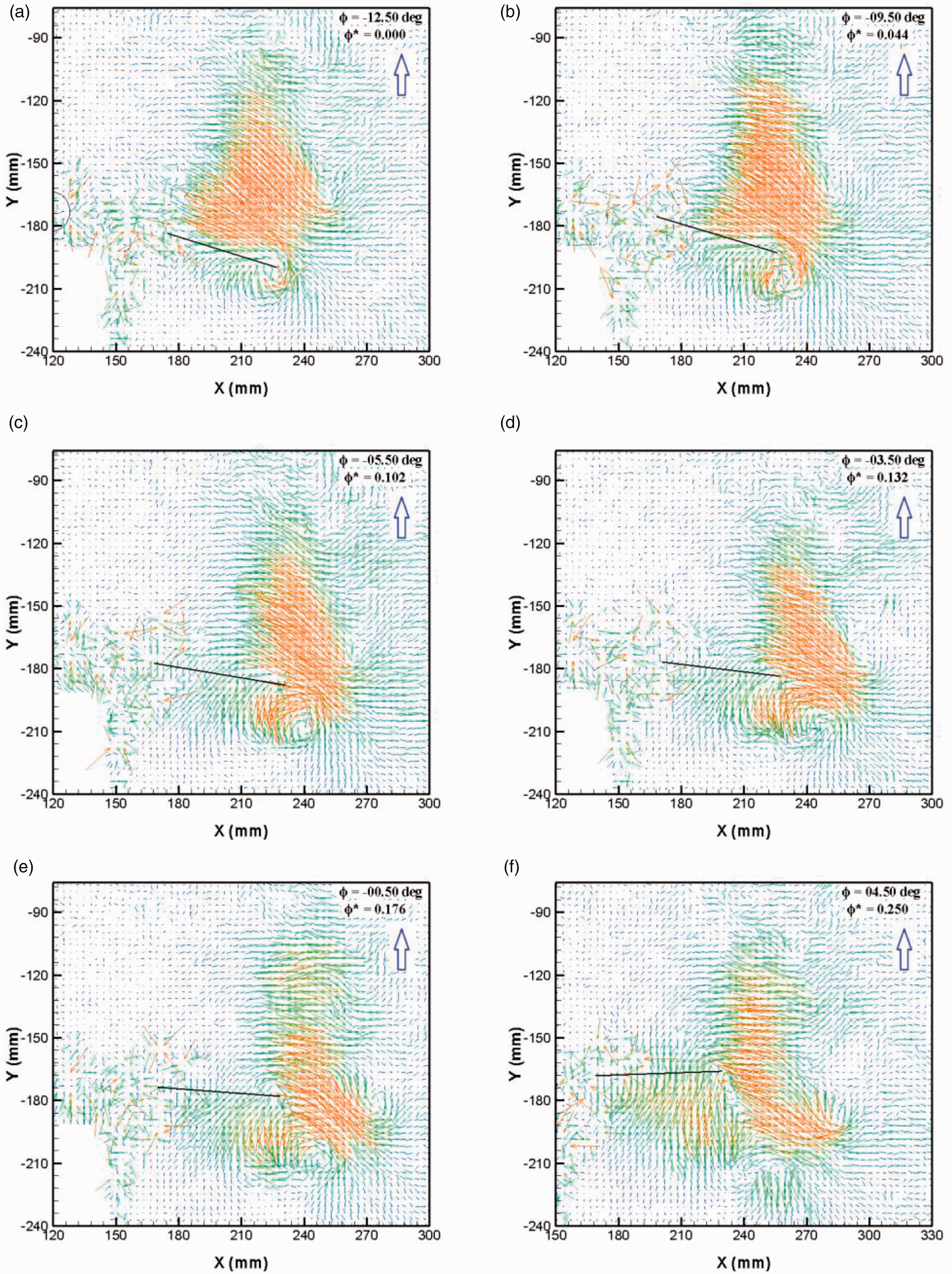
Figure 11 shows the velocity field during the US of the flapping cycle. At the beginning of the US when ϕ = −12.5°, streamwise flow on upper surface toward wing tip, formation of tip vortex of opposite nature to that at beginning of DS, the jet-like flow some distance above the upper surface of wing toward the wing tip and a few weak counter rotating vortices some distance to the right upper side of the wing tip are visible. The flow features are not exactly mirror image of those at the beginning of DS due to the asymmetry in the angular orientation of the wing from the horizontal axis in the two cases.

From ϕ = −12.5° to ϕ = −9.5° it is observed that the wing-tip vortex grows in size and gets detached from the wing. The upward movement of the wing induces the jet stream to rapidly move toward the wing tip and beyond. The counterpart vortices (same direction) get merged into a single structure; they grow larger in size and move away from the wing. Their dynamics is largely influenced by the jet.

From ϕ = −9.5° to ϕ = −5.5° it is found that the detached tip vortex interacts strongly with the jet and tends to get stretched. A spanwise flow along wing upper surface exists toward wing tip from the beginning of the US to this angle range.

For the angle range ϕ = −5.5° to ϕ = −0.5° the wing-tip vortex gets further stretched and the counter rotating vortex continues to grow in size and moves further away from the wing in the downward direction along with a bifurcated jet stream. The wing-tip vortex and counter rotating vortex approach each other and move further away from the wing tip.

The suction effect on the lower surface of the wing grows stronger due to its acceleration and induces a near normal flow toward the surface for ϕ = −0.5° to ϕ = 4.5°. Pockets of vortices are observed in the shear layer formed along the path followed by the wing tip. This shear layer lies at the interface of the upward moving flow induced by the wing motion and the downward moving flow carrying a pair of counter rotating vortex and bifurcated jet.

As the ϕ increases from 4.5° to 15.5° the upward moving flow toward wing lower surface increases substantially and gets almost isolated from the downward moving flow which moves further away from the wing making the shear layer wider.

From ϕ = 15.5° to ϕ = 29.5° the downward flow with a pair of counter rotating vortex and bifurcated jet move further downward and far from the wing to have any significant effect. This region can be considered to be the end of wake capture effect during US. The flow dragged by the wing increases in extent and forms the dominant flow feature.

In the final leg from ϕ = 29.5° to the end of the US, the large region of flow that is being dragged by the wing tends to get divided into two regions. The bifurcation is distinctly visible from ϕ = 39.5° onwards. One region continues to follow the wing which tends to form the tip vortex right at the end of the US and which is visible at the beginning of the subsequent DS. The other region moves along a right upwardly direction and rolls to form a vortex toward the right side of the wing. This is the counter rotating vortex which is visible in the beginning of the subsequent DS.

Vorticity and λ₂ criterion

The present section exhibits the flow features like co-rotating vortices, counter rotating vortices, bound vortex, and their strength and interactions by superimposing vorticity and λ₂ criterion.

Vorticity contours based on the definition ${\omega }_z=\left(\frac{\partial v}{\partial x}-\frac{\partial u}{\partial y}\right)$ , where clockwise (CW) vorticity, which satisfies the condition ω_z<0, has been represented by dotted contours and counter clockwise (CCW) vorticity, which satisfies the condition ω_z>0, has been represented by continuous contours.

Vortex identification method proposed by Jeong and Hussian, ³⁹ which is called as λ₂ criterion has been used to identify the swirling zones or vortex structures and shearing zones in the flow field

$${\lambda }_2={\left(\frac{\partial u}{\partial x}+\frac{\partial v}{\partial y}\right)}^2-4\left(\frac{\partial u}{\partial x}\frac{\partial v}{\partial y}-\frac{\partial u}{\partial y}\frac{\partial v}{\partial x}\right)$$

(7)

Negative and positive values of λ₂ correspond to swirling (represented by dark/gray color in the figures) and shearing (represented by white color in the figures) regions of the flow, respectively. In Figure 21 of Appendix 1, color contour figure is shown for a particular flapping angle as an example to indicate the range of λ₂ magnitudes. Spatial derivatives have been calculated by second-order accurate central difference scheme.

From Figure 12, at the beginning of the down stroke at ϕ = 54.5° two counter rotating vortices are visible near the wing tip. It is evident that the wing-tip vortex in DS (WTV1) is stronger than the CW one, secondary weak vortex (SWV). Bound vortices of CCW and CW nature are visible both on the lower as well as on the upper side of the wing. The bound vortex on the lower surface is distinctly stronger than its counterpart on the upper surface. A pocket of CW vortices exists above the bound CCW vortex on the upper surface. A CW vortex is seen at near about one span distance toward the right of the wing tip which has a higher strength (in magnitude) than the co-rotating vortex near wing tip (SWV) but lower strength than that of the WTV1. This CW vortex would henceforth be referred as “far away CW vortex” (FACW). Pockets of vortices are also visible at wing root but they are not of significant strength.

Figure 12.

Vorticity (line contours) and ${\lambda }_2$ criterion (gray contours) during DS of flapping cycle for case I: AR 1.5 and f at 1.5 Hz.

At ϕ = 52.5° the wing-tip vortex pair (WTV1 and SWV, counter rotating pair) grows in size but reduces in strength. The bound vortex existing on the lower surface of the wing stretches out toward the wing tip and loses strength but keeps feeding the WTV1. The CW vortices existing above the bound vortex on upper surface of wing grow both in size and strength. The FACW vortex which is now approximately at a unit span length to the right of the wing tip grows in size but loses strength. Small pockets of vortices of opposite nature which are in close proximity are found to interact and grow in strength in the neighborhood of FACW vortex.

At ϕ = 50.5° merging of the CCW bound vortex with the WTV1 enables it to grow in size and strength and finally get detached from the wing tip. The SWV tends to follow a similar trajectory as the CCW detached tip vortex and grows in strength which may be due to the heavy shear existing within the small gap between the WTV1 and SWV pair. FACW vortex further loses strength but the small neighboring vortex gains strength through interaction.

Around ϕ = 47.5° the wing-tip vortex grows much larger and loses some strength. The SWV seems to split into two parts. The bound vortex near wing tip regains strength. The FACW is about to merge with a neighboring co-rotating vortex which was formed earlier through interaction of smaller vortex pairs.

At ϕ = 44.5° bound vortex from wing tip gains strength and forms a shear layer which rolls up toward wing-tip vortex which has stretched significantly and lost strength. The portion of the split SWV which was nearer to the wing-tip vortex continues to roll around it but loses strength whereas its other portion gets disintegrated. The merged FACW vortex grows stronger.

Between ϕ = 44.5 and 36.5°, the wing tip shear layer seems to undergo KH instability due to the increased effective velocities thereby forming a stream of smaller chunks of vortices instead of a stable shear layer. The disintegrated portion of the wing-tip vortex merges with smaller vortex structures of the same kind in its neighborhood and gains strength. FACW loses strength from ϕ = 44.5 to 41.5° and gains strength from ϕ = 41.5 to 36.5°.

At around ϕ = 36.5° the bound CCW vortex on upper surface has almost moved away by feeding to the wing tip shear layer making way for the CW vortex pocket which was earlier existing above it to come closer to the upper surface of the wing.

Between ϕ = 36.5 and 31.5°, small pockets of CW vortices are seen near to the right side of the wing tip with reasonable strength. The FACW keeps growing in strength and convects away from the wing tip. The vortex structures formed due to KH instability seem to get further scattered in the wing wake. At ϕ = 31.5° the FACW is surrounded by multiple counter rotating vortices of smaller size.

Between ϕ = 31.5° and the end of the DS, the CW vortex pockets existing above the wing seem to get bound to it and gain in size and strength. Between ϕ = 26.5° and the end of the DS, the FACW continues to lose strength and convects further away from the wing. Over an angle range of ϕ = 36.5 to −11.5° some coherent vortex structures emerging out of the scattered vorticity formed due to KH instability are seen in the wing wake.

From ϕ = 11.5° till the end of the DS, small regions of CCW vortices are found to be distributed around the path followed by the wing tip and their strength seems to vary temporally.

In Figure 13, at the beginning of the US at ϕ = −12.5° a wing-tip vortex in US (WTV2) is visible at the wingtip along with bound vortex across the wing of the same nature. A strong CCW vortex is visible at approximately half span length distance in the upper right side of the wing. These are the residuals of vortex structures formed during DS. Small pockets of CCW vortices are visible in the far field. All CCW vortices are essentially the residuals from the previous DS.

Figure 13.

Vorticity (line contours) and ${\lambda }_2$ criterion (gray contours) during US of flapping cycle for case I: AR 1.5 and f at 1.5 Hz.

At ϕ = −9.5° WTV2 continues to grow in size, lose strength, and move further away from the wing tip. Bound vortex of similar nature exists across the wing. The strong CCW vortex which would henceforth be referred as FACCW loses its strength and travels downwards.

At ϕ = −5.5 to −0.5° the wing-tip vortex grows in size and similar nature of bound vortex comes toward the wing tip to feed it. FACCW moves toward the wing-tip vortex. CCW bound vortex is initiated in the wing root. Small pockets of CCW vortices still exist in the far field.

From ϕ = −0.5 to 11.5° wing-tip vortices form continuously and they reattach with previously formed vortices forming a vortex street which does not follow the wing tip path but moves in the outboard direction. The counter rotating pair of FACCW and CW rotating wing-tip vortex move together with significant strength. The FACCW strength is higher than any other vortices in the flow field. Small pockets of CCW vortices come closer to the wingtip. The CCW bound vortex has grown in size and stretches the entire wing length.

At ϕ = 15.5° the counter rotating and co-rotating vortices interact to form smaller vortices. The vortex pair still remains and the wing-tip vortex formation continues.

From ϕ = 15.5 to 29.5° the wing-tip vortex grows in size, the vortex structure remains attached to the tip but swings upwards. Bound vortex gains strength. All remaining vortices are very weak. The wing tip and bound vortex are the dominant coherent structures.

From ϕ = 29.5° to end of US the wing-tip vortex intermittently grows and decays because as it grows bigger, some portion of it breaks away. When breakage occurs, one portion of the vortex remains attached to the wingtip while the other breaks and moves outboard. Counter rotating bound vortex grows in size and strength and specifically at the end of the stroke the bound vortex has higher strength at the tip. This bound vortex creates the WTV1 in the subsequent DS.

Comparison of flow field behavior

In “Velocity vector field” and “Vorticity and λ₂ criterion” sections, the velocity field and vorticity with λ₂ contours, respectively, have been discussed for case I: AR 1.5, f = 1.5 Hz for complete flapping cycle. In the present section, the comparison of flow field behavior across the four cases (I–IV) has been discussed.

For all the cases, during the DS or US a wing-tip vortex forms in the inboard direction which is CCW or CW in nature, respectively. The wing-tip vortices generated at the beginning of DS and US are represented as WTV1 and WTV2, respectively. It is a well-established fact that these vortices would contribute to generation of forces. Bound vortex is the feeding mechanism for the wing-tip vortex in either of the strokes. The bound vortex is caused due to spanwise flow over the wing, which travels from root to tip. In flapping wing fluid dynamics, the spanwise flow has been considered to play significant role in lift generation. ¹¹ Bound vortex is therefore of the same sign as the corresponding wing-tip vortex. The counterpart (countersigned bound vortex) starts growing from the wing root and moves from root to tip during the DS to generate wing-tip vortex at the beginning of the US. During the US this mechanism operates in a similar manner. This means two countersigned bound vortices move along the wing surface from root to tip, the one which is closer to the wing tip feeds to the wing-tip vortex, while the other which is forming from the root region feeds the wing-tip vortex in the following stroke. During the DS, the bound vortex structures develop on the upper surface of the wing, while in the US they develop in the lower surface of the wing. A similar phenomenon has been reported by Kim and Gharib. ⁴⁰ Therefore, it may be conjectured that bound vortex is the mother of wing-tip vortex and wing-tip vortex is the mother of other coherent structures formed in the flow field predominantly in the wing tip and adjoining regions.

It has been observed that there is a certain extent of flow in the immediate vicinity of the wing which tends to follow it or gets dragged by it. The mass of this flow which follows the wing is known as added mass. In the present study, the added mass flow starts developing during the course of DS or US which bifurcates from mainstream flow to form countersigned vortex (FACW or FACCW) at the end of DS or US, respectively. Therefore, the two vortices (wing-tip vortices—WTV1 or WTV2 and countersigned vortices—FACW or FACCW) which form a pair of counter rotating vortices are visible at the beginning of US or DS. This counter rotating vortex is caused by the residual flow generated during the previous stroke. The counter rotating vortex pair generated during US moves in a nearly horizontal direction whereas for DS it moves in a nearly vertical direction. This is because of the effect of kinematic asymmetry in the flapping mechanism. It may be worthwhile to recall that the kinematic asymmetry implies unequal upper and lower half stroke angles as mentioned in the “Procedure” section. The flow features for a given AR display very similar characteristics irrespective of flapping frequency. Kim and Gharib ⁴⁰ reported that the counter rotating vortex which they referred as stopping vortex (in the present case FACW and FACCW) has effect on force generation.

Vortex filamentation and fragmentation has been observed during the DS and US, respectively. Continuous ejection of vortices from wing tip has been noticed during the entire DS. In the later part of DS, small pockets of vortices along the wing tip path have been noticed. These are formed from the added mass due to KH instability. The vortices merge/amalgamate and form an elongated vortex sheet. This process is termed as filamentation. During US the filamentation process continues but the vortex sheet is less robust. It interacts with residual structures which aid its disintegration. This process or state of breaking down of an organized vortex sheet into smaller fragments is referred to as fragmentation. The vortex filamentation and fragmentation phenomena have been observed consistently for all the cases addressed in the present study. Figures for case II–IV are not included for the sake of brevity while case I was discussed in the “Velocity vector field” and “Vorticity and λ₂ criterion” sections. In order to provide a generic picture of the flow features for DS and US, schematic diagrams are shown in Figure 14.

Figure 14.

Schematic diagram of flow features for (i) DS and (ii) US of flapping cycle (red and black color indicates clockwise and counter-clockwise direction, respectively). FACW and FACCW: the residual vortical structures in clockwise and counter-clockwise direction, respectively; WTV1: wing-tip vortex in DS; WTV2: wing-tip vortex in US.

In addition to that, it has been found that wing–wake interaction is significant at the beginning of each stroke where counter rotating vortex pair is visible; this has been reported extensively in literature. End of wake capture for all the cases during DS and US has been observed approximately around ϕ* = 0.35 and 0.45 (for details regarding normalized flapping angle, see equation (6)), respectively.

Circulation

Figure 15 shows the size of the domain R² considered for calculation of circulation and subsequent analysis. The same domain size has been fixed for all the four cases (I–IV). This is the minimum region within which most of the dominant coherent structures are observed or perturbations are significant. In the region beyond this domain, the velocity field is found to be nearly stationary. This is established through PIV data. The red line indicates the top and bottom most positions of the wing during a typical flapping cycle (details shown in Table 2).

Figure 15.

Schematic of flapping domain for analysis (dimensions in mm).

The total circulation, Γ is obtained from the following equation (8) for the two-dimensional domain discussed above. The variation of circulation over the entire flapping cycle is shown in Figure 16 for all the cases. The circulation for the all four cases is found to be nearly conserved. Thereby, the Kelvin circulation theorem is expected to be by and large satisfied in the given circumstances. Further, it is expected that the effect of viscous and nonconservative forces would be minimum in a global sense even though there are localized regions where these effects are nontrivial. It may be pertinent to mention here that the flow field predominantly exhibits two-dimensional character in the mid chord plane since onset of three-dimensional instabilities is generally accompanied by nonconservation of circulation based on two-dimensional flow field information. ⁴¹ This section has been used as a basis for the subsequent sections (“Strain rate and rotation rate” and “Enstrophy”)

$$\Gamma ={{\displaystyle \iint }}^{\text{}}{\omega }_z\text{d}A$$

(8)

Figure 16.

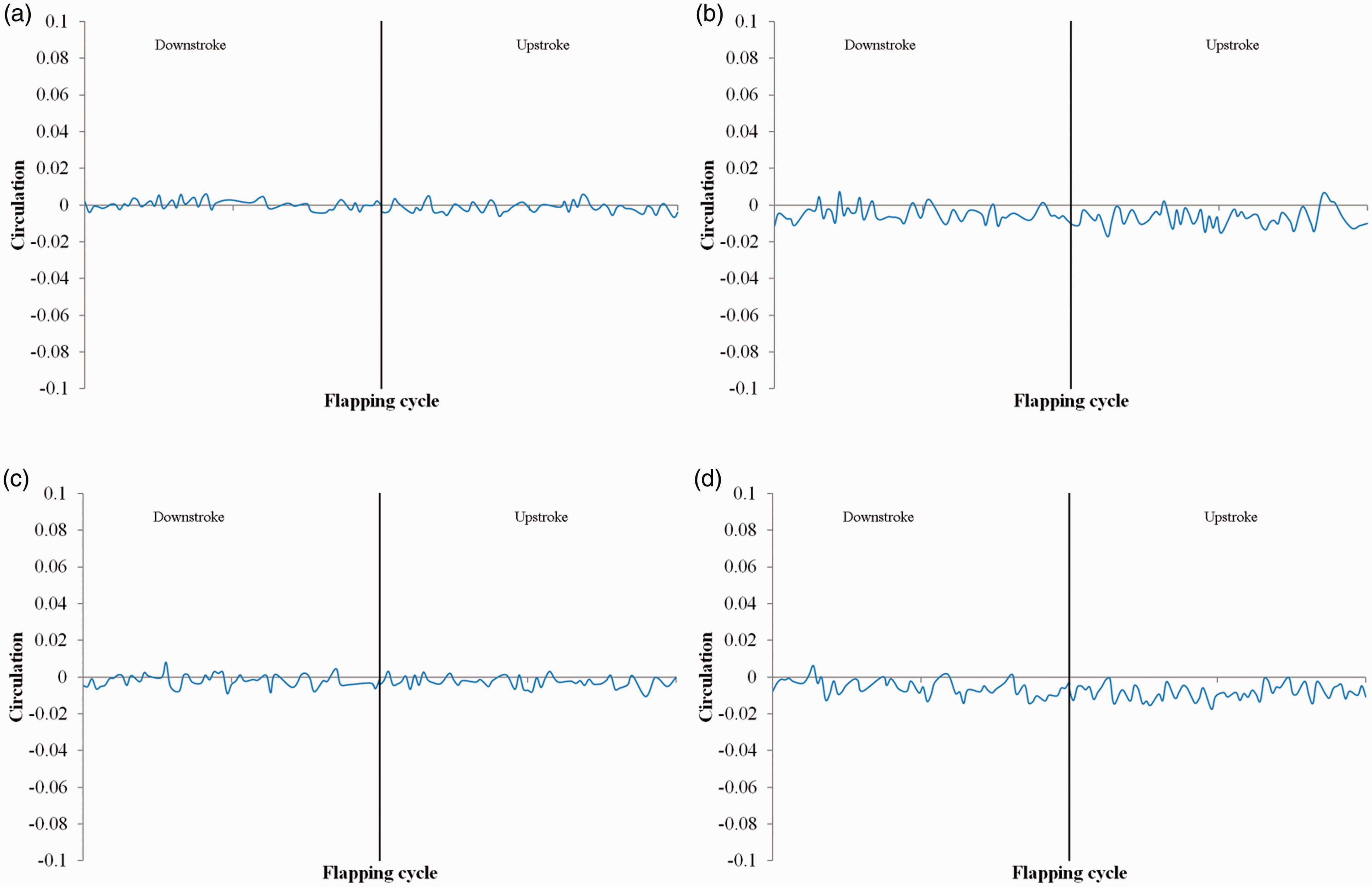
Circulation variation for (a) Case I: AR 1.5 and f at 1.5 Hz, (b) Case II: AR 1.0 and f at 1.5 Hz, (c) Case III: AR 1.5 and f at 2.0 Hz, and (d) Case IV: AR 1.0 and f at 2.0 Hz.

Strain rate and rotation rate

According to Wiess, ⁴² for an inviscid two-dimensional incompressible fluid flow, the vorticity gradients would tend to grow rapidly in that part of the fluid domain where squared magnitude of the rate of strain exceeds the squared magnitude of the rate of rotation. When the opposite relation exists between the above two quantities the vorticity gradients will behave in a periodic manner. It has been shown further that when the strain rate exceeds the rotation, the fluid is in a hyperbolic mode of motion which is characterized by strong shearing of vorticity field, whereas, when the rotation exceeds the strain the fluid is in an elliptical mode of motion that advects the vorticity smoothly. As a consequence of the above phenomenon, the vorticity gradients tend to concentrate in the regions of hyperbolic motion or the large-scale eddy structures. Similar observations have been reported by Herring ⁴³ and Bourguigonon and Brezis ⁴⁴ for an enclosed fluid domain, i.e. in a global sense as in the present case.

In the present section, the velocity gradient tensor $\frac{\partial u_i}{\partial x_j}$ has been decomposed into symmetric and antisymmetric parts known as strain rate tensor (S_ij) and rotation rate tensor (Ω_ij), respectively. At this point it may be worthwhile to recall that in the present study, two-dimensional planar view of the mid chord section of rigid main flapping wing has been considered. Though the flow field around the wing is actually three-dimensional in nature emphasis has been laid on studying the two-dimensional flow field characteristics at midsection of wing. Therefore, only the gradients of u and v components of velocity would figure in the strain rate tensor and rotation rate tensor

$$S_{\mathit{ij}}=\frac{1}{2}\left(\frac{\partial u_i}{\partial x_j}+\frac{\partial u_j}{\partial x_i}\right)\text{ and }{\Omega }_{\mathit{ij}}=\frac{1}{2}\left(\frac{\partial u_i}{\partial x_j}-\frac{\partial u_j}{\partial x_i}\right)$$

(9)

Spatial derivatives in the above equations have been calculated by using second-order central difference scheme. The components of the rate of strain tensor (S_ij) and rate of rotation tensor (Ω_ij) have been calculated for all pixels in a PIV image for a given wing orientation and stroke direction. Subsequently, these components are being used to compute the inner products of the tensors at each pixel. The inner products are then summed over the entire domain R² shown in Figure 15 to obtain the respective budgets of S² and Ω² (Figure 17). These budgets would be referred henceforth as strain rate squared and rotation rate squared, respectively. This exercise has been repeated for all angular orientations of the wing during a full stroke cycle. The distance between pixels has been mentioned earlier in the “PIV system and data processing” section. The present experiments are conducted with water which can be considered as incompressible and viscosity effects are negligible as is evident from the estimate of circulation reported in the “Circulation” section. Therefore, the present data closely conforms to two-dimensional incompressible inviscid fluid flow.

Figure 17.

Comparison of strain rate squared (S²) and rotation rate squared (Ω²) for (a) Case I: AR 1.5 and f at 1.5 Hz, (b) Case II: AR 1.0 and f at 1.5 Hz, (c) Case III: AR 1.5 and f at 2.0 Hz, and (d) Case IV: AR 1.0 and f at 2.0 Hz.

Figure 17 shows the comparison of strain rate squared (S²) and rotation rate squared (Ω²) for the entire flapping cycle. For case I, strain rate dominates over rotation rate at the beginning of DS and at the end of US. At the end of DS and beginning of US, rotation dominates over strain. For these wing orientations, a street of vortical coherent structures are visible above the wing as shown in figures 12 and 13 in the “Vorticity and λ₂ criterion” and “Comparison of flow field behavior” section. Case III has a similar behavior as case I but the gap between strain rate and rotation rate has been reduced for almost the entire cycle. The budgets for case III are higher than that of case I because of higher flapping frequency. For both cases I and III, the rise and fall of strain and rotation appears to be in phase for most part of the flapping cycle except for the later part of US where strain dominates over rotation. For case II and IV, rotation rate dominates over strain rate for most of the flapping cycle only apart from small portions at the beginning of DS and end of US. Two strong peaks are visible at beginning of DS and right at the end of US for case IV. The budgets for case II and IV (low AR wings, AR 1.0) are lower than those of case I and III (high AR wings, AR 1.5).

Figure 18 shows the difference between budgets of strain rate squared and rotation rate squared. If the difference is positive, it indicates global hyperbolic behavior, while if it is negative, it indicates global elliptic behavior of the flow field. For higher AR wings (case I and case III), hyperbolic behavior is predominant except for end of DS and beginning of US where elliptic behavior is seen. For lower aspect wings (case II and case IV), elliptic behavior is predominant except for beginning of DS and end of US where hyperbolic behavior is seen. The hyperbolic behavior becomes stronger at higher frequency.

Figure 18.

((S²)–(Ω²)) distribution for (a) Case I: AR 1.5 and f at 1.5 Hz, (b) Case II: AR 1.0 and f at 1.5 Hz, (c) Case III: AR 1.5 and f at 2.0 Hz, and (d) Case IV: AR 1.0 and f at 2.0 Hz.

Enstrophy

The enstrophy transport equation can be obtained by taking a dot product of the vorticity transport equation and it is represented as follows

$$\begin{array}{l}\frac{D}{\mathit{Dt}}\left(\frac{{\omega }^2}{2}\right)={\omega }_i{\omega }_j{S}_{\mathit{ij}}-\nu {\left(\nabla \times \omega \right)}^2\\ \hspace{1em}\hspace{1em}\hspace{1em}\hspace{1em}\hspace{1em}+\nabla \cdot \left[\nu \omega \times \left(\nabla \times \omega \right)\right]\end{array}$$

(10)

There are three source terms on the right-hand side of the above equation. It is discussed in Davidson ³³ that usually the third source term which is the divergence term is negligible. The first two source terms are, namely the vortex stretching or compression term and enstrophy dissipation term which is linked with the viscous effect. In fully developed turbulence, the entire range of vorticity coexists in the flow field starting from the integral scales to the Kolmogorov microscales. In the present problem, the integral scale is associated with flapping wing dimensions while the microscale depends on the Reynolds number associated with the flapping. The vortex stretching phenomenon dominates over vortex compression such that the net effect of the strain field is to create enstrophy. The interplay between the production of enstrophy through vortex stretching and destruction through viscous dissipation leads to temporal and spatial modulation of enstrophy which is represented through its substantial derivative. When enstrophy generation dominates over enstrophy dissipation it leads to time rate of enstrophy growth and vice versa. Enstrophy production is governed by the cosines of the alignment angle between the vorticity vector and the principal axes of the rate of strain tensor. ⁴⁵ In the present study, only the ω_z component of the vorticity vector can be accounted since the other components are not observable using x–y planar view of the mid chord section of the wing. Hence the interpretations that follow are restricted to the available planar data. A more complete understanding can be attained only through volumetric information which is beyond the scope of the present study.

In the present study, enstrophy budget (EN) is defined as the area integrated value of square of the z-component of vorticity

$$\mathit{EN}={{\displaystyle \iint }}^{\text{}}{\omega }_z^2\text{d}A$$

(11)

The integration has been performed over a two-dimensional domain as shown in Figure 15. Enstrophy distribution for the entire flapping cycle is obtained for all the four cases which is presented in Figures 19 and 20. A sixth-order polynomial fit has been used for smoothing the exact data shown in Figure 19 to obtain Figure 20. The smoothed curves are better suited for obtaining the important trends linked with frequency and AR change.

Figure 19.

Enstrophy variation for (a) Case I: AR 1.5 and f at 1.5 Hz, (b) Case II: AR 1.0 and f at 1.5 Hz, (c) Case III: AR 1.5 and f at 2.0 Hz, and (d) Case IV: AR 1.0 and f at 2.0 Hz.

Figure 20.

Comparison of enstrophy variation for all four cases.

For all four cases, enstrophy fluctuations have been noticed both in the DS and US similar to those reported in Ortega et al. ⁴¹ Forcing of the flow field by the flapping wing leads to continuous vortex formation, interaction, and dissipation which affect the vorticity magnitudes locally and enstrophy budget globally. Average enstrophy values for all four cases have been calculated for the entire cycle and compared. The values in descending order are 17.97 (case III), 15.72 (case IV), 13.96 (case I), and 13.59 (case II), respectively. From these values it is evident that higher frequencies produce higher enstrophy budgets and play a more dominant role than AR in determining the budget.

Closer scrutiny of Figures 19 and 20 leads to some more observations as follows:

For case I, some weak intermittent enstrophy peaks are visible at the beginning and end of the DS. There are some intermittent variations of enstrophy during US and the mean enstrophy reduces marginally.

For case II, the mean enstrophy increases marginally during DS. Sustained peaks are visible at the beginning of the US. However, the mean enstrophy reduces subsequently during major portion of the US.

Fairly strong sustained enstrophy peaks are visible at the beginning and end of both DS and US for case III. At the intermediate phase range, the mean enstrophy remains stable.

Some discrete enstrophy peaks are visible at the beginning and end of both DS and US for case IV. These peaks are comparable with case III; however, they are more intermittent for case IV. In the intermediate phase range, the mean enstrophy remains stable during DS but reduces during US.

It may be recalled that strain operates on the vorticity field leading to enstrophy production as represented by the first source term of the enstrophy equation. Strong vorticity and accompanying strain generated during beginning and end of DS and US at higher frequency is responsible for producing the enstrophy peaks for case III and IV, with more sustained strength observed for AR = 1.5 wing. Viscous dissipation is not strong enough to offset this effect. Vortex filamentation seems to be playing an active role in generating enstrophy during the entire DS to balance the dissipation. On examining Figure 17 in this light it can be inferred that for cases III and IV the interaction between strain and vorticity field is favorable which leads to production of enstrophy peaks. On the contrary, toward the end of US for case I, the interaction is unfavorable leading to lower enstrophy values.

Revisiting the second source term of the enstrophy equation it is observed that the viscous dissipation seems to be more active during the US where reduction of mean enstrophy takes place for case I and case II. It is observed that the reduction is larger for lower AR wing. Vortex fragmentation may be playing a role in the reduction of enstrophy. Due to fragmentation phenomenon vorticity gets more widely distributed in the smaller length scales at which viscous dissipation becomes active. Case III is able to counter this effect most effectively due to the dual advantage of higher AR and higher frequency. For all other cases, there is a decrease in enstrophy during US.

Conclusions

In the present study, flow field around rigid flat plate wings executing main flapping motion was studied using phase-locked two-dimensional PIV measurements. Two different AR (1.5 and 1.0) rectangular wings at 1.5 and 2.0 Hz flapping frequency in hovering flight mode and chord-based Reynolds number of the order of 10⁴ were studied covering a total of four different cases.

Vortex filamentation and fragmentation phenomena were observed during flapping cycle consistently for all the four cases irrespective of AR or frequency.

Distribution of global strain rate squared and rotation rate squared was used to distinguish the hyperbolic and elliptic nature of flow field. For higher AR wing, hyperbolic behavior was predominant except for end of DS and beginning of US where elliptic behavior was observed. For lower AR, wing elliptic behavior was predominant except for end of US and beginning of DS where hyperbolic behavior was seen. The hyperbolic behavior became stronger at higher frequency.

From enstrophy distribution it was evident that higher frequencies produce higher enstrophy budgets and play a more dominant role than AR in determining the budget. Enstrophy production seems to be correlated with the vortex filamentation process while enstrophy dissipation seems to be correlated with the vortex fragmentation process.

It is worth noting that while the budgets provide us information about overall nature of the flow field, they are not sufficient to analyze local flow properties very effectively. For example, a flow field exhibiting global hyperbolic behavior may exhibit local elliptic behavior in certain regions of the flow and vice versa.

The current study highlighted the existence of vortex filamentation and fragmentation phenomena in flow field around a rigid wing in main flapping motion irrespective of AR and frequency, while effect of change in flapping frequency and AR became visible through the various budgets like square of strain, rotation, and their difference as well as enstrophy.

The practical implications of the present study are summarized below. In MAV/MUWV the designer would consider the type of kinematics, flapping frequencies, materials, etc. for a given application. From the outcomes of the present work, for the given kinematics and operating conditions, some major design inputs may be drawn for developing flapping wing models as follows (a) Use of one degree flapping mechanism^{10,11,15–17,21,26} can reduce the overall weight of the flying vehicles because the number of linkages and cranks required in the present case are minimum. (b) In order to attain desired flapping frequency for a given AR within the parametric domain, the power requirements from the present study would be useful for estimation in designing the flying model. (c) In the present experiments, it was observed that the time taken during the DS was lesser than US. Zhu and Zhou, ²⁹ Wang et al., ³⁰ Sarkar and Venkatraman, ³¹ and Sarkar et al. ³² reveal that time asymmetry in flapping is expected to produce higher force. Therefore, flapping mechanism design may be optimized to achieve time asymmetry so that desired forces are produced during the strokes. (d) Inertial load and added mass along with AR, materials, and frequency effect play a vital role in attaining the design flapping amplitudes.^15–17 This becomes a significant challenge when the vehicle is functioning in a heavier fluid like water. The present study produced data of actual achievable amplitudes for the given kinematics and operating conditions in water. This would be an important input for designing and building MUWV models of comparable scale for missions involving vertical movement through the depth of water for surveillance, reconnaissance, scientific exploration, etc. When the present study is extended to airborne flapping wing vehicles it is expected that variation in flapping amplitude would occur to a much lesser extent due to significantly lower density of the medium compared to water. (e) The 1:3 angular asymmetry kinematics used in the present mechanism would enable production of vertically upward force in the given orientation. Complex missions may require thrust vectoring which can be achieved if the flapping mechanism can be gimbaled. Additionally, if flexible wings are deployed, they would assist in producing forward motion. (f) From flow field data, since the vortex filamentation and fragmentation phenomena are found to be consistent for all four cases considered, the pattern of vertical force generation is expected to be similar within the investigated parametric domain. (g) From strain rate, rotation rate, and enstrophy it can be anticipated that higher flapping frequencies and higher AR wing would produce higher normal force.

If the results of the current work are applied to practical models, it is anticipated that common flow field phenomena and similar trend in upward forces would be produced even if marginal variation in wing AR and flapping frequency occurs. Therefore, results of this study can be applied to design vehicles for missions which predominantly require upward movement. Future scope of the current research includes force/moment measurements, elaborate parametric studies, and conducting the experiments in air. Further analysis of the unsteady flow field around a flapping wing with particular emphasis on tracking the evolutionary cycle of specific coherent structures would be useful.