Numerical investigation of the low-frequency flow oscillation over a NACA-0012 aerofoil at the inception of stall

Abstract

High-fidelity large eddy simulation is carried out for the flow field around a NACA-0012 aerofoil at Reynolds number of $9\times {10}^4$ , Mach number of 0.4, and various angles of attack around the onset of stall. The laminar separation bubble is formed on the suction surface of the aerofoil and is constituted by the reattached shear layer. At these conditions, the laminar separation bubble is unstable and switches between a short bubble and an open bubble. The instability of the laminar separation bubble triggers a low-frequency flow oscillation. The aerodynamic coefficients oscillate accordingly at a low frequency. The lift and the drag coefficients compare very well to recent high-accuracy experimental data, and the lift leads the drag by a phase shift of $\pi /2$ . The mean lift coefficient peaks at the angle of attack of $10.25°$ , in total agreement with the experimental data. The spectra of the lift coefficient does not show a significant low-frequency peak at angles of attack lower than or equal the stall angle of attack ( $10.25°$ ). At higher angles of attack, the spectra show two low-frequency peaks and the low-frequency flow oscillation is fully developed at the angle of attack of $11.0°$ . The behaviour of the flow-field and changes in the turbulent kinetic energy over one low-frequency flow oscillation cycle are described qualitatively.

Introduction

Recently, the low Reynolds number aerodynamic, ${10}^4\le {\text{Re}}_c\le {10}^6$ , has received much attention due to the increasing interest in the aerodynamic performance of unmanned and micro-air vehicles (UAVs and MAVs) especially when aerofoil stall is likely expected by the influence of the laminar separation bubble (LSB). Low Reynolds number is achieved due to flying at high altitude, where the kinematic viscosity increases, and small geometrical dimensions. Other examples of low Reynolds number aerodynamic are found in the operation of turbine cascades, wind turbines, and flight of birds and insects. Historically, high Reynolds number aerodynamics ( ${\text{Re}}_c>{10}^6$ ) has been studied extensively, and a large experimental and numerical data are available. The main difference between the high and the low Reynolds number aerodynamics is represented in different physical behaviours of the flow, such as the formation of the LSB and the low-frequency flow oscillation phenomenon (LFO). In most high Reynolds number flow cases, the turbulent boundary layer takes place over a long portion of the aerofoil chord, where the flow undergoes transition to turbulence near the aerofoil leading edge. Turbulence causes the flow to be energetic and remain attached to the surface until it eventually separates at high angles of attack. In contrast, at low Reynolds number, a laminar boundary layer takes place near the leading edge, which can cause separation due to the adverse pressure gradient (point S in Figure 1). The transition location moves further downstream, and subsequently the flow reattaches to the surface (point R in Figure 1). The resultant structure is the LSB which is constituted between points S and R in Figure 1.

Figure 1.

A short bubble over a NACA-0012 at ${\text{Re}}_c=9\times {10}^4$ and the angle of attack of $11.0°$ .

Aerofoil stall is the abrupt drop in the lift when the critical angle of attack, i.e., the angle of the maximum lift, is exceeded. The stall characteristics are essential to the design of wings and final selection towards a particular performance criterion. Therefore, many studies were carried out to gain insight into the stall phenomenon. Both the leading edge and the thin aerofoil stall types are markedly affected by the formation of the LSB. Therefore, it is essential to understand the behaviour of the LSB before any attempt to understand and control the stall phenomenon. For this purpose, several studies have been carried out such as Owen and Klanfer ¹ , Crabtree ² , Gaster ³ , Young and Horton ⁴ , Horton^5,6 and Roberts. ⁷

Melvill Jones ⁸ was the first to observe the LSB. After that, a series of experiments were carried out by Young and Horton ⁴ to investigate the structure of the LSB. Horton ⁶ described the time-averaged structure of the LSB as shown in Figure 1. The laminar boundary layer separates at point S, undergoes transition to turbulence, and reattaches at point R. The flow domain between these two points is split into two regions, the free shear layer and the recirculating bubble. These two regions are divided by the mean dividing streamline (line $S-T\prime -R$ ). The bubble is bounded by the mean dividing streamline and the aerofoil surface (line $S-T-R$ ). The free shear layer starts laminar in the vicinity of the aerofoil leading edge and becomes turbulent downstream point $T\prime$ . ⁷

Gaster ³ investigated the structure and stability of the LSB. He invented a brilliant model that allowed him to collect data for various LSBs and derive a bursting criterion for the LSB. At near stall conditions, the LSB becomes unstable. The short bubble abruptly bursts and forms a long bubble. Figure 1 shows a short bubble formed over a NACA-0012 at ${\text{Re}}_c=9\times {10}^4$ and the angle of attack of $11.0°$ . The length of the bubble is of about 20% of the chord length. Figure 2 shows an open bubble formed as a consequence of the bursting of the short bubble. The aerodynamic coefficients oscillate accordingly at a low frequency. The unsteadiness of the LSB causes the LFO phenomenon which could sometimes be observed near stall conditions. The first to observe and document this phenomenon was Zaman et al. ⁹

Figure 2.

An open bubble over a NACA-0012 at ${\text{Re}}_c=9\times {10}^4$ and the angle of attack of $11.0°$ .

Zaman et al. ⁹ investigated the LFO phenomenon experimentally and numerically for the flow field around 2–D aerofoil models at low chord Reynolds numbers in the range of $1.5\times {10}^4-3\times {10}^5$ . The authors defined the LFO phenomenon in terms of Strouhal number ( $\mathit{St}=\mathit{fcsin}(\alpha )/U_{\infty }$ ). Where f is the flow oscillation frequency, c is the length of the aerofoil chord, α is the angle of attack, and $U_{\infty }$ is the free-stream velocity. The frequency of oscillation is considered to be low if St < 0.2, which exists in bluff-body shedding. The authors used velocity spectra to find the frequency of the LFO phenomenon. Furthermore, the authors studied the fluctuation of the lift coefficient, where it has a quasiperiodic trend between stalled and non-stalled conditions. For the numerical study, the authors used a thin layer approximation to solve 2–D Navier–Stokes equations using Baldwin–Lomax turbulence model. The authors studied the effect of the grid size on the fluctuations of the lift coefficient and verified it with experimental data. The authors concluded that the LFO phenomenon occurs when there is a trailing edge stall or a thin aerofoil stall. Bragg et al. ¹⁰ investigated, experimentally, the flow field around an LRN(1)-1007 aerofoil at ${\text{Re}}_c$ in the range of $3\times {10}^5-1.25\times {10}^6$ and α in the range of $0°-28°$ . The LFO phenomenon is captured using hot-wire spectra measurements in the aerofoil wake where the LFO phenomenon is observed in the interval $14.4°\le \alpha \le 16.6°$ . The authors reported that the Strouhal number increases slightly with the Reynolds number and significantly with the angle of attack. The Strouhal number associated with the oscillation is lower by approximately 10 times than the Strouhal number of bluff-body shedding. The surface–oil flow and laser sheet visualisation experiments showed the growth and bursting of the leading-edge separation bubble and its role in the flow oscillation. Also, the authors discussed the possible relation between the shear layer flapping and the flow oscillation and suggested that it should be further investigated.

Broeren and Bragg ¹¹ utilised the aerofoil used in Bragg et al. ¹⁰ at ${\text{Re}}_c=3\times {10}^5$ and $\alpha =15°$ . They used conditionally averaged laser Doppler velocimetry (LDV) to resolve a fully separated boundary layer. The flow separates due to the merging of the leading edge and the trailing-edge separation regions when they grow in time. Also, their data showed the periodic switching between stalling and non-stalling behaviour, which involved a leading-edge separation bubble, and how the bubble interacted with the trailing-edge separation. Broeren and Bragg ¹² studied five different aerofoil configurations (NACA-2414, NACA-64A010, LRN-1007, E374 and Ultra-Sport) by measuring the wake velocity across the spanwise direction, and using mini-tufts for flow visualisation. The authors reported that all the stall types are dependent on the type of the aerofoil. They concluded that the LFO phenomenon always occurs in the aerofoils that exhibit a thin aerofoil stall or a combination of both thin aerofoil and trailing-edge stall which is in agreement with Zaman et al. ⁹

Tanaka ¹³ performed an experimental study of the flow field around a NACA-0012 aerofoil using particle image velocimetry (PIV) measurements to capture the LFO phenomenon near stall conditions. He investigated the flow at a chord Reynolds number of $1.3\times {10}^5$ for a range of angles of attack around $11.5°$ . His results showed that the frequency of fluctuation increases, in the range of 1.5–3 Hz, as the angle of attack increases, in the range of $11.3°-12°$ . While at $\alpha =11.5°$ the amplitude is greatest and the fluctuation is quasiperiodic. Also, he noticed a formation of a large vortex near the leading edge when the flow is separated from the surface. This vortex bends the shear layer and introduces the free stream to the separated region. Thus, this vortex is responsible for the switching of the flow between a separated and an attached phase. Rinoie and Takemura ¹⁴ studied a similar experiment to that of Tanaka ¹³ for a flow over a NACA-0012 aerofoil at Reynolds number of $1.3\times {10}^5,\alpha =10°$ and $11.5°$ , to investigate the mechanism behind the LFO phenomenon. The authors observed a steady short bubble near the leading edge with a length of approximately 10% of the chord length at $\alpha =10°$ . Moreover, in the time-averaged flow, they detected a long bubble with a length of 35% of the chord at $\alpha =11.5°$ . At this angle of attack, the flow is oscillating at about 2 Hz between the short bubble near the leading edge and a fully separated flow.

One of the first attempts to capture the LFO phenomenon using Large Eddy Simulation (LES) was carried out by Mary and Sagaut, ¹⁵ but they did not capture it. After that, Mukai et al. ¹⁶ carried out an LES to study the flow around an LRN(1)-1007 aerofoil at Reynolds number of $3\times {10}^5$ and Mach number of 0.1. The authors used two types of mesh and two different dimensions for the width of the aerofoil in the spanwise direction to investigate the LFO phenomenon near stall conditions. They found that the LFO phenomenon takes place at $\alpha =15.35°$ . The authors reported that their results were in good agreement with those of the experimental work of Broeren and Bragg ¹⁷ and Broeren and Bragg. ¹¹ The LFO is captured and shown in the time history of the lift coefficient. The quasiperiodic cycle of the LFO is presented, and the dominant Strouhal number is 0.024 which is comparable to the Strouhal number of 0.023 in the experimental measurements. Furthermore, LES results were more realistic than the RaNS results when they were compared to the experimental data for the mean lift coefficient. Sandham ¹⁸ used a time accurate viscous–inviscid interaction method (VII) for the coupled potential flow and integral boundary-layer equations to study several aerofoil models near stall conditions. He modelled the laminar–turbulent transition by an absolute instability which sustains the transition of the LSB without using any upstream perturbations. The Strouhal number of the LFO was found to be dependent on the shape of the aerofoil. The author showed that the LFO phenomenon could be captured by a simple model of boundary layer transition because the bubble bursting occurred as a consequence of potential flow/boundary layer interactions. Almutairi et al. ¹⁹ carried out an LES to study the low Reynolds flow ( $\mathit{Re}=5\times {10}^4$ ) around a NACA-0012 aerofoil at $\alpha =5°$ . The main objective was to check the validity of the LES method by comparing their results with the Direct Numerical Simulation (DNS) results documented by Jones et al. ²⁰ Furthermore, They studied the effect on the numerical accuracy by using the mixed time scale (MTS) model as a subgrid-scale model (SGS). They increased the domain in the spanwise direction which resulted in matching results with the DNS results. Afterwards, Almutairi and Alqadi ²¹ investigated the phenomenon of natural LFO using the method used by Almutairi et al. ¹⁹ The authors studied numerical simulations of the flow field around a NACA-0012 aerofoil at Reynolds number of $5\times {10}^4$ , Mach number of 0.4, and four angles of attack at near stall conditions ( $9.25°,9.29°,9.4°$ , and $9.6°$ ). The authors found that self-sustained natural LFO is observed for all the angles. Also, they showed the quasiperiodic cycle for the lift coefficient which agrees with the experimental observations and measurements of Tanaka ¹³ and Rinoie and Takemura. ¹⁴ Almutairi et al. ²² used the method which has been verified by Jones et al. ²⁰ and Almutairi et al. ¹⁹ They performed an LES of the flow field around a NACA-0012 at $\mathit{Re}=1.3\times {10}^5$ and $\alpha =11.5°$ . The authors described the role of transition and how the three-dimensional large scales structures are broken down to small scales, which are followed by turbulent region. The authors showed the oscillation of the time histories of the lift, the drag, and skin-friction coefficients in a quasi-periodic manner which is an indication of the LFO phenomenon. They found that the dominant Strouhal number is 0.00826 which is comparable to the St = 0.008 of the experimental work of Rinoie and Takemura. ¹⁴ However, the grid they used is relatively coarse in the transition region, especially in the spanwise direction ( $\Delta z^{+}>40$ ) and in the wall-normal direction ( $y^{+}>1$ ).The authors concluded that the flow oscillation occurred due to strong trailing-edge vortex shedding that generates acoustic waves when the flow is separated. The acoustic waves travel upstream, energies the separated shear layer, and force the flow to reattach. The authors reported that the strong vortex shedding at the trailing-edge dies down during the attached phase of the flow, therefore, the flow separates again. The stability of the LSB and the underlying mechanism behind its associated LFO have been investigated extensively; however, very little of the general character is known about the mechanism that triggers the instability of the LSB, and generates the LFO phenomenon.

Recently, Eljack ²³ carried out a high-fidelity numerical simulation to investigate the LSB and its associated LFO phenomenon over a NACA-0012 aerofoil at ${\text{Re}}_c=5\times {10}^4$ and various angles of attack around the onset of stall. He showed that at low angles of attack the LSB is present and intact, at moderate angles of attack the LSB becomes unstable and the flow-field switches between an attached phase and a separated phase at low frequency. At relatively high angles of attack, he showed that the LSB becomes an open bubble that leads the aerofoil into a full stall. Eljack et al. ²⁴ used the data sets generated by Eljack ²³ to characterise the flow-field. The authors verified and validated the LES data, then used a conditional time-averaging to describe the flow field in detail and investigate the effects of the angle of attack on the characteristics of the flow field. They reported the existence of three distinct angle-of-attack regimes. At relatively low angles of attack, flow and aerodynamic characteristics are not much affected by the LFO. At moderate angles of attack, the flow field undergoes a transition regime in which the LFO develops until it reaches a quasiperiodic switching between separated and attached flow. At high angles of attack, the flow field and the aerodynamic characteristics are overwhelmed by a quasiperiodic and self-sustained LFO until the aerofoil approaches the angle of full stall. The authors concluded that most of the observations reported in the literature about the LSB and its associated LFO are neither thresholds nor indicators for the inception of the instability, but rather are consequences of it. Eljack and Soria ²⁵ utilised the conditional time-averaging used by Eljack et al. ²⁴ and a conditional phase-averaging to reveal the underlying mechanism that generates and sustains the LFO phenomenon. The authors showed that a triad of three vortices, two co-rotating vortices (TCV) and a secondary vortex counter-rotating with them is behind the quasiperiodic self-sustained bursting and reformation of the LSB and its associated LFO phenomenon. They reported that a global oscillation in the flow field around the aerofoil is observed in all of the investigated angles of attack, including at zero angle of attack. The authors found that when the direction of the oscillating flow is clockwise, it adds momentum to the boundary layer and helps it to remain attached against an Adverse Pressure Gradient (APG) and vice versa. Eljack and Soria ²⁶ applied dynamic mode decomposition (DMD) and proper orthogonal decomposition (POD) to investigate the dynamics of the flow field. The authors identified three distinct dominant flow modes: a globally oscillating flow mode at a low frequency; a locally oscillating flow mode on the suction surface of the aerofoil at a low frequency and a locally oscillating flow mode along the wake of the aerofoil at a high frequency. The authors discussed the dynamics of the flow in detail, determined the root causes that trigger the instability of the LSB, and revealed the underlying mechanism behind the LFO phenomenon. However, the authors explained that at such low Reynolds number the LSB is less coherent and the LFO cycle is disturbed. Thus, similar investigation at a higher Reynolds number is merited. The present work takes up Eljack ²³ ’s work and investigates the flow field past a NACA-0012 aerofoil at Reynolds number of $9\times {10}^4$ , Mach number of 0.4 and various angles of attack around the onset of stall.

Mathematical modelling

In the present study, the fluid flow is governed by the viscous-compressible Navier–Stokes equations. The non-dimensional analysis of these equations is achieved using the following non-dimensional variables

$$u_j=\frac{u_j^{*}}{u_r^{*}},\rho =\frac{{\rho }^{*}}{{\rho }_r^{*}},T=\frac{T^{*}}{T_r^{*}},x_j=\frac{x_j^{*}}{c},\mu =\frac{{\mu }^{*}}{{\mu }_r^{*}}$$

$$P=\frac{P^{*}}{{\rho }_r^{*}{u}_r^{*2}},t=\frac{t^{*}{u}_r^{*}}{c}$$

where

$$u_j=\left[\begin{array}{c}u\\ v\\ w\end{array}\right]\text{ and }{x}_j=\left[\begin{array}{c}x\\ y\\ z\end{array}\right]$$

Here, ρ, T and μ are the fluid density, temperature and dynamic viscosity, respectively. P is the flow pressure, t is time and c represents the aerofoil chord length. The subscript r denotes the reference variables, and the symbol $*$ indicates the dimensional variables. The reference variables for the non-dimensional analysis are: $u_r^{*}={\rho }_r^{*}=T_r^{*}=c={\mu }_r^{*}=1$ .

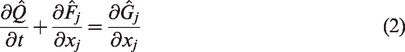
The non-dimensional form of the three-dimensional compressible Navier–Stokes equations can be written in vector form as

$$\frac{\partial Q}{\partial t}+\frac{\partial F_j}{\partial x_j}=\frac{\partial G_j}{\partial x_j}$$

(1)

where

$$Q=\left[\begin{array}{c}\rho \\ \rho u\\ \rho v\\ \rho w\\ \rho (D+E)\end{array}\right],F_j=u_{j}Q+\left[\begin{array}{c}0\\ {\delta }_{1j}P\\ {\delta }_{2j}P\\ {\delta }_{3j}P\\ P{u}_j\end{array}\right]$$

and

$$G_j=\left[\begin{array}{c}0\\ {\sigma }_{1j}\\ {\sigma }_{2j}\\ {\sigma }_{3j}\\ {\sigma }_{\mathit{kj}}{u}_k-b_j\end{array}\right]$$

where $D=\frac{T}{\gamma (\gamma -1)M_{°}^2}$ and $E=\frac{1}{2}{u}_j.u_{\mathit{j}}^T$ .

Q is a vector including the conservative flow variables, F is the filtered inviscid flux vector and G is the filtered viscous flux vector. σ_ij is the viscous stress tensor, and the term b_j is given by

$$b_j=\frac{\mu \left(T\right)}{\left(\gamma -1\right)Pr\mathit{Re}{M}_{\infty }^2}\frac{\partial T}{\partial x_j}$$

and

$$J=\frac{\mu \left(T\right)}{\left(\gamma -1\right)Pr{\text{Re}}_c{\text{M}}_{\infty }^2}$$

where ${\text{M}}_{\infty }=0.4$ is the reference Mach number, $\gamma =1.4$ is the specific heat ratio, ${\text{Re}}_c=9\times {10}^4$ is the chord Reynolds number and Pr = 0.72 is the Prandtl number, respectively. The dynamic viscosity μ is calculated using the dimensionless form of Sutherland’s law

$$\mu \left(T\right)=T^{\frac{3}{2}}\frac{1+C}{T+C},C=0.3686$$

The relation between T, ρ and P is given by the ideal gas law

$$T=\gamma M_{\infty }^2\frac{P}{\rho }$$

The free-stream pressure estimated using the above relation is equivalent to 4.464. The viscous stress tensor σ_ij is given by

$${\sigma }_{\mathit{ij}}=\frac{\mu \left(T\right)}{\mathit{Re}}\left(\frac{\partial u_i}{\partial x_j}+\frac{\partial u_j}{\partial x_i}-\frac{2}{3}{\delta }_{\mathit{ij}}\frac{\partial u_k}{\partial x_k}\right)$$

where, δ_ij is the Kronecker delta.

For LES, any flow variable q is decomposed for large and small scales, therefore, $q=\overline{q}+q\prime$ . $\overline{q}$ and $q\prime$ represents the large and small scales, respectively. For compressible flow, it is convenient to use $\tilde{q}=\overline{\rho q}/\overline{\rho }$ as a Favre filtered flow variable (density weighted). By applying the Favre filtering to equation (1), the resultant filtered form is given by

$$\frac{\partial \widehat{Q}}{\partial t}+\frac{\partial \widehat{F_j}}{\partial x_j}=\frac{\partial \widehat{G_j}}{\partial x_j}$$

(2)

where

$$\widehat{Q}=\left[\begin{array}{c}\overline{\rho }\\ \overline{\rho }\tilde{u}\\ \overline{\rho }\tilde{v}\\ \overline{\rho }\tilde{w}\\ \overline{\rho }(\tilde{D}+\tilde{E})\end{array}\right],\widehat{F_j}=\widetilde{u_j}\widehat{Q}+\left[\begin{array}{c}0\\ {\delta }_{1j}\overline{P}\\ {\delta }_{2j}\overline{P}\\ {\delta }_{2j}\overline{P}\\ \overline{P}{\tilde{u}}_j\end{array}\right]$$

and

$$\widehat{G_j}=\left[\begin{array}{c}0\\ {\widehat{\sigma }}_{1j}-{\tau }_{1j}\\ {\widehat{\sigma }}_{2j}-{\tau }_{2j}\\ {\widehat{\sigma }}_{3j}-{\tau }_{3j}\\ {\widehat{\sigma }}_{\mathit{kj}}{\tilde{u}}_k-{\widehat{b}}_j\end{array}\right]$$

where $\tilde{D}=\frac{\tilde{T}}{\gamma \left(\gamma -1\right)M_{°}^2}$ and $\tilde{E}=\frac{1}{2}{\tilde{u}}_j.{\tilde{u}}_j^T$

$${\widehat{b}}_j=\tilde{J}\frac{\partial \tilde{T}}{\partial x_j}$$

$$\tilde{J}=\frac{\tilde{\mu }\left(T\right)}{\left(\gamma -1\right)Pr{\text{Re}}_c{\text{M}}_{\infty }^2}$$

$$\mu \left(\tilde{T}\right)={\tilde{T}}^{\frac{3}{2}}\frac{1+C}{\tilde{T}+C},C=0.3686$$

$$\tilde{T}=\gamma M_{\infty }^2\frac{\overline{P}}{\overline{\rho }}$$

$${\widehat{\sigma }}_{\mathit{ij}}=\frac{\mu (\tilde{T})}{\mathit{Re}}\left(\frac{\partial {\tilde{u}}_i}{\partial x_j}+\frac{\partial {\tilde{u}}_j}{\partial x_i}-\frac{2}{3}{\delta }_{\mathit{ij}}\frac{\partial {\tilde{u}}_k}{\partial x_k}\right)$$

The SGS stress tensor τ_ij expresses the effect of small scales on the residual stress, and it is modelled as follows

$${\tau }_{\mathit{ij}}=\overline{\rho }(\widetilde{u_i{u}_j}-{\tilde{u}}_i{\tilde{u}}_j)$$

(3)

The models used in the present study are based on the idea of an eddy viscosity ν_t. Consequently, the stress tensor is given by

$${\tau }_{\mathit{ij}}-\frac{1}{3}{\delta }_{\mathit{ij}}{\tau }_{\mathit{kk}}=2{\nu }_t{\tilde{S}}_{\mathit{ij}}$$

τ_kk is the isotropic part of the τ_ij and the strain rate tensor is defined by

$${\tilde{S}}_{\mathit{ij}}=\frac{1}{2}\left(\frac{\partial {\tilde{u}}_i}{\partial x_j}+\frac{\partial {\tilde{u}}_j}{\partial x_i}\right)$$

By applying the dimensional analysis to ν_t, it gives

$${\nu }_t\propto I_{\mathit{SGS}}{u}_{\mathit{SGS}}$$

(4)

where I_SGS and u_SGS are the length and velocity scales for the unresolved motion, respectively. Several models are developed to describe the effect of the SGS stress components. The MTS model was developed by Inagaki et al. ²⁷ This model is constructed without using any explicit wall damping function to overcome the drawbacks of other SGS models. In the MTS model, the expression of ν_t which is given in equation (4) is modified to be given by

$${\nu }_t\propto T_{\mathit{SGS}}{u}_{\mathit{SGS}}^2$$

where T_SGS is a time scale, and u_SGS is a velocity scale, which can be calculated using

$$u_{\mathit{SGS}}^2={(\overline{u}-\widehat{\overline{u}})}^2$$

where a top hat filtering ( $\widehat{\hspace{0.17em}}$ ) denotes a second filtering process. By applying this formula, the ν_t approaches zero in the laminar flow region because the u_SGS also approaches zero and the flow is fully resolved. This can be considered as an important benefit of using the MTS model since it does not need any additional damping functions. The term T_SGS is given by

$$T_{\mathit{SGS}}^{-1}={\left(\frac{\overline{\Delta }}{u_{\mathit{SGS}}}\right)}^{-1}+{\left(\frac{{\text{C}}_{{\text{}}_{\text{t}}}}{\left|\overline{S}\right|}\right)}^{-1}$$

where $\overline{\Delta }$ represents the filter size and ${\text{C}}_{{\text{}}_{\text{t}}}$ is a fixed parameter (in the current study ${\text{C}}_{{\text{}}_{\text{t}}}=10$ ). Inagaki et al. ²⁷ suggested the time scale as $1/\left|\overline{S}\right|$ . They found that ${\nu }_t\propto u_{\mathit{SGS}}^2/\left|\overline{S}\right|$ exhibits a good agreement with other SGS models that have a wall damping function, but it was not appropriate to implement this eddy viscosity in a region away from the wall where the problem of dividing by zero can arise. This problem was solved by adding another time scale $\overline{\Delta }/u_{\mathit{SGS}}$ , which was proposed by Yoshizawa et al. ²⁸ Therefore, the ν_t can be expressed as follows

$${\nu }_t={\text{C}}_{{\text{}}_{\text{MTS}}}{T}_{\mathit{SGS}}{u}_{\mathit{SGS}}^2$$

where ${\text{C}}_{{\text{}}_{\text{MTS}}}$ is a fixed model parameter (in the current study ${\text{C}}_{{\text{}}_{\text{MTS}}}=0.03$ ).

There are two methods to overcome grid to grid oscillations. The first method is by adding an artificial dissipation to Navier–Stokes equations. The second method is by applying a filter to the flow-field for the small scales without disturbing the large scales. In the current study, latter method is used. Visbal and Rizzetta ²⁹ found that to maintain numerical stability, it is convenient to use compact schemes of order equal or greater than the order of spatial discretisation. The spatial filtering is applied using explicit low-pass filter to the unfiltered field to obtain an approximate solution.

$${\alpha }_f{\overline{\widehat{Q}}}_{i-1}+{\overline{\widehat{Q}}}_i+{\alpha }_f{\overline{\widehat{Q}}}_{i+1}={\displaystyle \sum _{n=0}^2\frac{a_n}{2}}\left({\widehat{Q}}_{i+n}+{\widehat{Q}}_{i-n}\right)$$

${\overline{\widehat{Q}}}_i$ and ${\widehat{Q}}_i$ are the filtered and unfiltered values at point i, respectively. α_f is a free parameter in the range of $0\le {\alpha }_f\le 0.5$ . The coefficients a_n are derived by matching with the corresponding Taylor series coefficients based on the order of accuracy. The low-pass and high-pass filters remove the small and large scales, respectively.

Almutairi ³⁰ studied six filter schemes. He used both spectral analysis and random field filtering where they gave consistent resolution characteristics of each filter scheme. Firstly, in the spectral analysis, the comparison criterion was the transfer function (TF). The results showed that fourth-order tridiagonal and pentadiagonal filters have the best spectral behaviour because they have a TF = 1 over the widest range of wavenumber. Secondly, he applied Fast Fourier Transformation (FFT) to random fields where the results showed that the shape of energy spectra for various low-pass filters is similar to the spectral behaviour in the previous method. Furthermore, the fourth-order tridiagonal and the fourth-order pentadiagonal filters have the superior performance on stretched grids. Therefore, a fourth-order tridiagonal filter is applied in the current study. It is unnecessary to implement the whole filtered function but a part of it according to the following equation

$$\overline{\overline{Q}}=\widehat{Q}-\sigma (\widehat{Q}-\overline{\widehat{Q}})$$

where $\overline{\overline{Q}}$ is the resulting filtered vector and σ is the filter constant between 0 and 1. If σ = 0 then no filtering is applied. In the present study $\sigma =0.25$ . The conservative flow-field variables are filtered in x, y and then z directions, respectively.

Computational setup

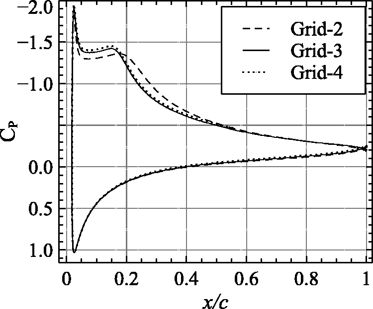
The computational domain and curvilinear coordinates system ( $\xi ,\eta$ and ζ) are illustrated in Figure 3. A NACA-0012 aerofoil is oriented at the angle of attack of $11.0°$ . The dimensions $W/c=5,L_{\eta }/c=7.3$ , and $L_{\zeta }/c=0.5$ refer to the wake length, the C-grid radius and the domain length in spanwise direction, respectively. It should be noted that all the dimensions are scaled by the aerofoil chord length where c = 1. An adequate grid resolution is required to resolve the large eddies in the flow field. The grid spacing in the viscous wall units y⁺, $\Delta x^{+}$ , and $\Delta z^{+}$ are estimated to examine the grid resolution in the wall-normal, streamwise, and spanwise directions, respectively. LES requires a wall-normal, streamwise and spanwise grid resolutions of approximately $y^{+}<1,\Delta x^{+}<30$ , and $\Delta z^{+}<20$ , respectively.

Figure 3.

The computational domain.

In the present study, four different C-grids are constructed with various distributions in $\xi ,\eta$ and ζ curvilinear directions. Different grid spacing is used to demonstrate the sensitivity of the flow field and the characteristics of the LSB to the grid distribution. The LSB formation, elongation and bursting should be well resolved, therefore, the grid resolution near the aerofoil surface, especially on the suction side, is critical. In Table 1, $N_{\xi },N_{\eta }$ and $N_{\zeta }$ are the grid points in ξ, η and ζ curvilinear directions, respectively. PS, SS NW, and total points refer to the number of grid points on the aerofoil pressure surface, suction surface the wake and the total number of grids in the domain, respectively. Figure 4 shows a close-up of the computational grid around the aerofoil at the angle of attack of $11.0°$ . The grid is generated using a hyperbolic grid generator, and the grid points are clustered near the surface. The grid is orthogonal with a minimum skewness throughout the computational domain. Grid–1 ( $637\times 320\times 86$ ) is an improved mesh distribution of the grid used by Almutairi and Alqadi. ²¹ The grid points in the wall-normal direction were changed to intensify grid points near the aerofoil surface and across the free shear layer. Grid–2 ( $780\times 320\times 125$ ) is a refined version of Grid–1 that was used by Eljack. ²³ The grid distribution on the suction surface of the aerofoil was made equidistant starting from the leading-edge to the mid-chord. Grid–3 ( $832\times 351\times 167$ ) is a refined version of Grid–2. The number of grid points in the wall-normal direction was increased to ensure high resolution at the aerofoil surface and across the separated shear layer. The number of grid points in the spanwise direction was also increased from 125 grid points in Grid–2 to 167 grid points in Grid–3. This has reduced the grid spacing in viscous wall units to less than 15 and significantly improved the solution. An adequate grid distribution in the spanwise direction is crucial for the break-down of the evolving Kelvin–Helmholtz instability. Thus, prediction of the correct location of transition depends primarily on the grid distribution. Grid–3 was further refined in the streamwise direction to obtain Grid–4 ( $1192\times 351\times 167$ ). The streamwise grid spacing in viscous wall units was reduced to less than 10.

Figure 4.

Computational grid at the angle of attack $\alpha =11.0°$ .

Table 1.

Computational grid parameters.

Grid	y +	$\Delta x^{+}$	$\Delta z^{+}$	$N_{\xi }$	$N_{\eta }$	$N_{\zeta }$	PS	SS	NW	Total points
Grid–1	>1	<50	<50	637	320	86	130	170	170	17,530,240
Grid–2	<1	<20	<20	780	320	125	130	251	201	31,200,000
Grid–3	<1	<15	<15	832	351	167	130	235	235	48,769,344
Grid–4	<1	<10	<15	1192	351	167	130	355	355	69,871,464

In this study, the Navier–Stokes equations were discretised using a fourth-order accurate explicit central difference scheme for the spatial discretisation of the internal points. The Carpenter fourth-order accurate scheme as outlined in Carpenter et al. ³¹ is applied to treat the points near the boundary.^30,32 The temporal discretisation was performed using a low-storage fourth-order Runge–Kutta scheme. The integral characteristic boundary condition is applied at the free-stream and far field boundaries. ³³ The zonal characteristic boundary condition is applied at the downstream exit boundary, ³⁴ which are considered as non-reflected boundary conditions to overcome the circulation effects at the boundaries. The solution stability was improved by implementing an entropy splitting scheme. ³⁵ The entropy splitting constant β was set equal to 2.0. ³² The adiabatic and no-slip conditions are applied at the aerofoil surface. The LSB, its associated LFO, and the flow field are inherently statistically two dimensional. Therefore, a periodic boundary condition is applied in the spanwise direction for each step of the Runge–Kutta time steps.

Results and discussion

In this study, LESs were carried out for the flow field around a NACA-0012 aerofoil at low Reynolds number of $9\times {10}^4$ , Mach number of 0.4 and the angles of attack of $10.0°,10.25°,10.4°,10.6°,10.8°,11.0°$ , and $11.2°$ . The free-stream direction is set parallel to the horizontal axis. The time step is set to ${10}^{-4}$ non-dimensional time unit. The computational domain was initiated with a clean free-stream conditions (u = 1, v = 0, w = 0, T = 1, and ρ = 1). The simulation was initiated without using flow forcing. Data sampling process started after the flow transition has decayed, and the flow becomes statistically stationary in time after 50 non-dimensional time units (500,000 time steps). Aerodynamic forces ( $C_L,C_D,C_m$ and $C_f$ ) were sampled continuously at a non-dimensional sampling frequency of 10,000, and for 250 non-dimensional time units. The velocity components, pressure and Reynolds stresses were sampled on the x–y plane. The data was ensemble-averaged in the spanwise direction and locally time-averaged every 50 time steps on the fly before it was recorded at a non-dimensional sampling frequency of 204. The sampled data spans 100 non-dimensional time units and covers four LFO cycles. The locally time-averaged and spanwise ensemble-averaged local pressure coefficient was sampled around the aerofoil surface at a non-dimensional sampling frequency of 204.

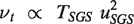
The distribution of the pressure coefficient on the suction surface of the aerofoil is dependent on the grid resolution as shown in Figure 5. However, the three grids produced similar solutions on the pressure surface of the aerofoil. Apparently, this is because the flow is laminar on this side of the aerofoil and the solution is less sensitive to the grid distribution compared to the suction surface. The coarse grid fails to capture small flow structures, and overestimates the dissipation of kinetic energy. Consequently, it affects the transition process, and underestimates the momentum available for the boundary layer to reattach the flow. Thus, the reattachment location takes place further downstream, and the bubble is longer than that produced using the fine grid. The mean flow was obtained on the x–y plane by time-averaging the sampled data. After that, the streamlines plot on the x–y plane was used to estimate the mean bubble size. The mean bubble size is found to be about 30% and 25% of the aerofoil chord length, for the coarse grid (Grid–2) and the fine grid (Grid–3), respectively. Grid–4 produced a bubble of almost the same size as that produced by Grid–3.

Figure 5.

Sensitivity of the mean pressure coefficient to grid refinement at the angle of attack $\alpha ={11.0}^{°}$ .

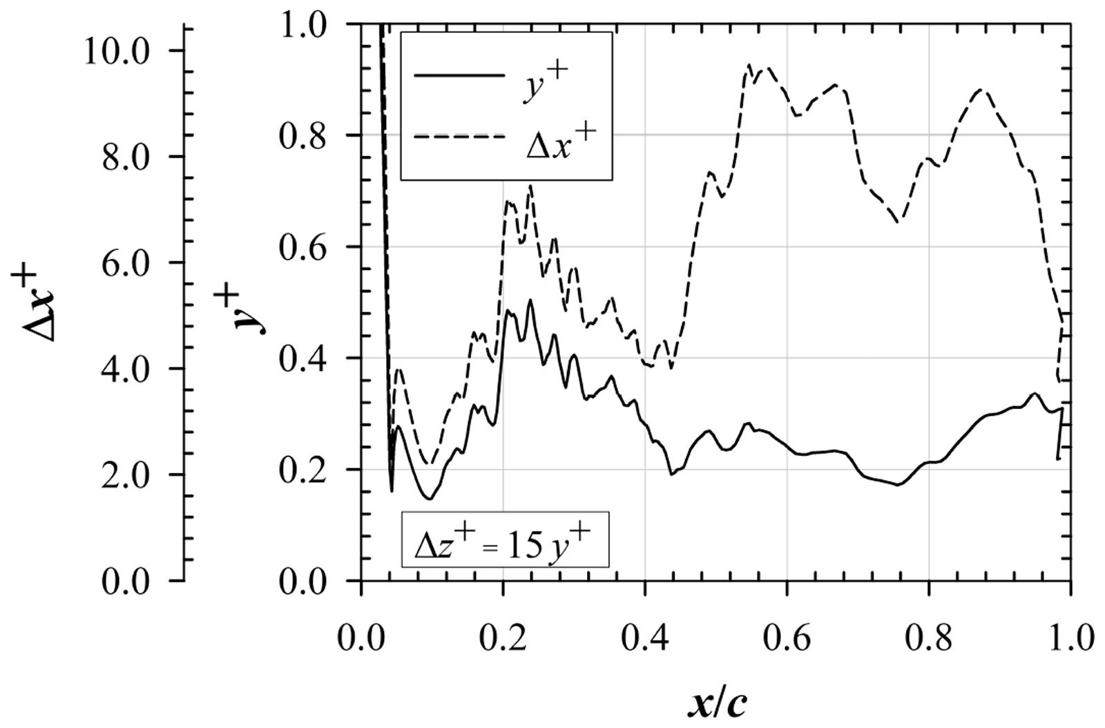
The grid spacing given in Table 1 is assumed to give the desired grid resolution. The actual grid spacing in viscous wall units is extracted from the LES data. Figures 6 and 7 show the grid spacing in viscous wall units on the suction surface of the aerofoil for both attached and separated phases of the flow, respectively. The grid spacing in the wall-normal direction is less than 1 ( $y^{+}<0.75$ ), as shown in the figures. The highest value of y⁺ exists in the transition region in the interval $0.1\le x/c\le 0.3$ . The maximum values of y⁺ are 0.68 and 0.5 for the attached and separated flow phases, respectively. The grid resolution in the streamwise direction is less than 15 ( $\Delta x^{+}<13.5$ ). An equidistance mesh is employed in the streamwise direction in the region $0.04\le \Delta x^{+}\le 0.4$ . This is the region where the transition process takes place. An adequate grid resolution in the transition region is highly recommended due to the unsteadiness of the shear layer and the development of the Kelvin–Helmholtz instability. The grid spacing in the spanwise direction is uniform ( $\Delta z=0.5/167$ ), and the value of $\Delta z^{+}$ is constant at $15y^{+}$ . It is noted that the values of y⁺ and $\Delta x^{+}$ for the separated flow phase are lower than those for the attached flow phase. This is due to the lower velocity gradient in the separated flow, which decreases the wall shear stress and consequently the y⁺ and $\Delta x^{+}$ .

Figure 6.

Grid resolution, attached phase.

Figure 7.

Grid resolution, separated phase.

The instantaneous iso-surface of λ₂–criterion ( ${\lambda }_2=-200)$ , coloured by the total energy per unit mass (E) is illustrated in Figure 8. The left side of the figure shows the early transition process where the shear layer is attached. The shear layer is a little bit distorted, and the two-dimensional rolls are converted to large three-dimensional structures followed by a breakdown process. Consequently, the flow becomes turbulent. The separated flow phase, the right side of Figure 8, shows a late transition process. In this process, the shear layer is detached from the surface towards the free stream, and the breakdown process of the two-dimensional scales moves downstream. Additionally, a strong vortical structure shedding is observed near the aerofoil trailing edge, for the separated flow. However, it becomes weaker for the attached flow. These figures show that, qualitatively, the flow field switches between an attached phase and a separated phase. Consequently, a low-frequency global oscillation in the flow field is triggered. The velocity components, the pressure and the aerodynamics coefficients oscillate accordingly at a low frequency.

Figure 8.

Instantaneous iso-surface of λ₂–criterion ( ${\lambda }_2=-200$ ) coloured by the total energy per unit mass (E).

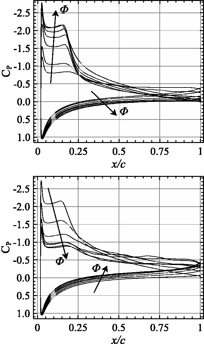
The pressure adjacent to the aerofoil surface oscillates due to the switching of the flow between an attached and separated phases. Consequently, the pressure coefficient oscillates in harmony with the global low-frequency flow oscillation. Most of the oscillations in the pressure coefficient take place on the suction surface of the aerofoil. The local instantaneous pressure coefficient is locally time-averaged at 12 phases covering the phase angles from $0°$ to $360°$ . Figure 9 shows the evolution of the pressure coefficient over one low-frequency cycle. As shown in the figure, the pressure decreases dramatically at the aerofoil leading edge due to the curvature of the aerofoil as the velocity tends to increase. After that, the pressure coefficient remains almost constant in the range $0.05\le x/c\le 0.2$ . This is indicative that the LSB is formed in this region. The pressure coefficient increases drastically downstream the LSB, building up an adverse pressure gradient, but the flow has enough momentum to overcome new separation.

Figure 9.

Locally averaged pressure coefficient at the phase angles of $\Phi =0^{°}$ – ${360}^{°}$ plotted versus the locations along the chord measured from the aerofoil leading edge. The arrows indicate the direction in which the phase angles increase in ascending order. The flow is fully attached at $\Phi ={180}^{°}$ , and is fully separated at $\Phi =0^{°}$ and ${360}^{°}$ .

At the phase angle of $0°$ , the spike of the pressure coefficient in the vicinity of the leading edge has the minimum magnitude compared to the peaks at other phase angles. The pressure coefficient is almost flat and has minimal amplitude. As the phase angle increases, the magnitude of the pressure coefficient increases on the suction surface of the aerofoil. The adverse pressure gradient is strengthened, the length of the LSB decreases, and the flow is attaching at higher phase angles. The adverse pressure gradient has the maximum amplitude, the LSB has the minimum length, and the flow is fully attached at the phase angle of $180°$ . After that, the process is reversed during the phase angles of $\Phi =180°$ – $360°$ as seen in the figure.

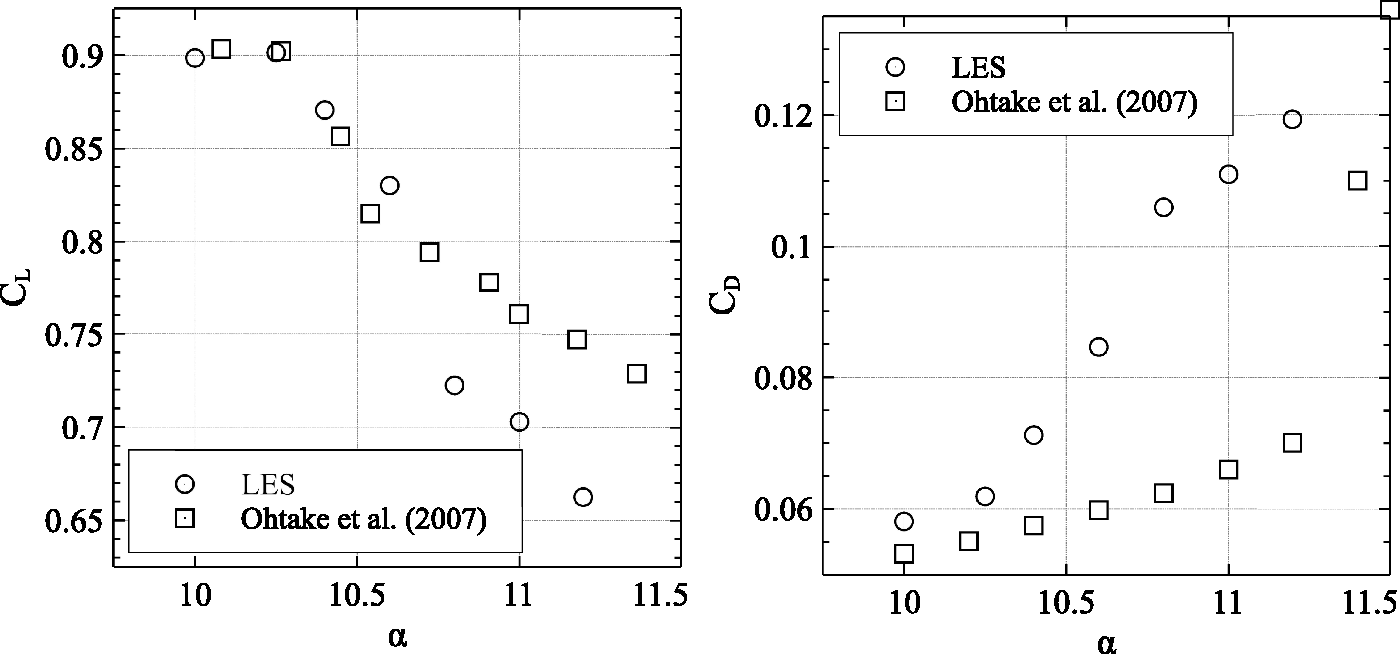
The pressure coefficient is duly integrated around the aerofoil surface to obtain the aerodynamic coefficients. The lift and the drag coefficients oscillate at a low frequency as seen in Figure 10. The horizontal dashed lines display the mean lift coefficient of 0.7224, 0.7028 and 0.6626 at the angles of attack of $10.8°,11.0°$ and $11.2°$ , respectively. The lift coefficient oscillates between a maximum value of about 0.9, when the flow is fully attached, and a minimum value of about 0.4 when the flow is fully separated as seen in the figure. Thus, the lift coefficient oscillates at an amplitude of about 35% of its mean value. At the angle of attack of $10.8°$ , the LFO cycle is disturbed, and only two or three cycles resemble each other in a time span of about 12 cycles. As the angle of attack increases to $11.0°$ , the LFO cycle becomes uniform and almost all of the cycles resemble each other. The LFO cycle becomes disturbed again when the angle of attack increases to $11.2°$ . This is indicative that the LFO is fully developed at the angle of attack of $11.0°$ . The dashed lines on the drag coefficient plots show the mean drag values of 0.1060, 0.1110 and 0.1193 at the angles of attack of $10.8°,11.0°$ and $11.2°$ , respectively. The LFO cycle itself is smoother, and the LSB is more coherent compared to the LFO cycle obtained at the Reynolds number of $5\times {10}^4$ by Eljack. ²³ The drag coefficient consistently peaks when the lift coefficient hits its mean value as seen in the figure. Thus, the lift coefficient is leading the drag coefficient by a phase shift of $\pi /2$ . This agrees with the observations of Eljack ²³ inequities of how disturbed the LFO cycle in his study is. The phase shift can also be noted in the work of Almutairi et al., ²² however, the authors did not discuss it. In the present study, Eljack ²³ study, and Almutairi et al. ²² work only the pressure component of the force is considered. Thus, no phase shift between the lift and the drag is expected. However, these are unsteady aerodynamics studies, and the oscillations in the aerodynamic coefficients are arisen from the oscillating pressure. The oscillating pressure is the sum of several modes and the most dominant are two low-frequency modes. The first low-frequency mode (LFO-mode-1) affects the lift coefficient, and the second low-frequency mode (LFO-mode-2) affects the drag coefficient. The LFO-mode-1 leads the LFO-mode-2 by a phase shift of $\pi /2$ , as discussed in Eljack and Soria. ²⁶ Thus, the lift leads the drag by a phase shift of $\pi /2$ . The lift and drag signals are time-averaged to obtain their mean values for all of the investigated angles of attack. The left-hand side of Figure 11 shows that the lift coefficient peaks at the angle of attack of $10.25°$ in total agreement with the high-accuracy recent experimental data of Ohtake et al. ³⁶ The circles display the mean lift coefficient estimated from the LES data, and the squares indicates the value of the lift coefficient transformed from the experimental data of Ohtake et al. ³⁶ using the Prandtl–Glauert transformation. ³⁷ The present study is carried out at Mach number of 0.4, whereas, the experiment was carried out at incompressible conditions. Thus, Prandtl–Glauert transformation was used to add the effects of compressibility to the experimental data both in term of the shift in the angle of attack and the magnitude of the lift coefficient. Reducing the Mach number of the numerical simulation to match that of the experiment would considerably increase the computational cost. At higher angles of attack, the lift coefficient drops rapidly and compares very well to the experimental data. However, at the angles of attack of $10.8°,11.0°$ and $11.2°$ the lift coefficient values estimated from the LES data are less than their corresponding experimental values. At these three angles of attack, the lift coefficient oscillates with a significant amplitude around its mean values as seen in Figure 10. Thus, a longer time record of the data is required to estimate the true mean. However, very long data sampling is not visible in numerical simulation. The right-hand side of Figure 11 shows the mean drag coefficient. The circles indicate the mean drag coefficient estimated from the LES data, the squares display the experimental data. The numerical simulation data mimic that of the experiment, however, the LESs overestimate the drag coefficient. The drag force is not defined for an inviscid flow, therefore, the Prandtl–Glauert transformation rule cannot be used to add effects of compressibility to the incompressible experimental data. Hence, the discrepancy between the LES and the experimental data is due to the effects of compressibility.

Figure 10.

Time histories of the lift and the drag coefficients for the angles of attack of $11.8°,11.0°$ and $11.2°$ .

Figure 11.

Mean lift and drag coefficients plotted versus the angle of attack. Circles: LES data; squares: experimental data Ohtake et al. ³⁶

A qualitative study is performed to characterise the unsteady behaviour of the LSB over one low-frequency cycle, and to show that the LFO is physically captured. The data is locally time-averaged over 12 subintervals. Each subinterval consists of 20,000 time steps, two non-dimensional time units, in the range $0°\le \varphi \le 360°$ with the interval of $30°$ . At the beginning of the cycle, at $\varphi =0°$ , the flow is fully separated, and the LSB becomes an open bubble that spans over one chord length as seen in Figure 12. At the phase angles of $\varphi =30°$ – $60°$ , the length of the open bubble reduces, and the flow field is attaching. At the phase angle of $\varphi =90°$ the open bubble disappears. A short bubble is formed in the vicinity of the leading edge, and a trailing-edge bubble is formed. The trailing-edge bubble diminishes in size and the short bubble preserve the same length at the phase angle of $\varphi =120°$ . The trailing-edge bubble vanishes, the short bubble has a minimum length, and the flow is fully attached at $\varphi =180°$ . The process is then reversed, and the LSB continues to increase in length with time until it bursts. The LSB forms an open bubble, and the flow becomes fully separated at $\varphi =330°$ .

Figure 12.

Streamlines of the flow field around the NACA-0012 aerofoil at the phase angles of $\Phi =0°$ – $330°$ .

The Reynolds stresses are locally time-averaged on the x–y plane over 12 subintervals covering one low-frequency cycle. The locally averaged Reynolds stresses are then used to calculate the Turbulent Kinetic Energy (TKE) using the equation $k=\frac{1}{2}(u^{\prime 2}+v^{\prime 2}+w^{\prime 2})$ . The location of the maximum TKE can be used as an indicator for the location of the transition. The TKE has significant magnitude along the separated shear layer on the suction surface of the aerofoil as seen in Figure 13. The TKE has its minimum values at the phase angle of $\varphi =0°$ where the flow field is fully separated as discussed before. At this phase angle, the shear layer moves away from the aerofoil surface. Thus, the location of the maximum TKE is located away from the aerofoil surface and further downstream ‘late-transition’. At higher phase angles, the magnitude of the TKE increases, and the location of its maximum magnitude moves towards the aerofoil surface and upstream. The maximum values of the TKE reach a maxima at the phase angle of $\varphi =180°$ where the flow is fully attached, the location of maximum TKE at its closet locations to the aerofoil surface and its furthest locations upstream. The process is reversed as the phase angle is further increased until the flow becomes fully separated at the phase angle of $\varphi =330°$ .

Figure 13.

Turbulent kinetic energy of the flow field around the NACA-0012 aerofoil at the phase angles of $\Phi =0°$ – $330°$ .

The spectra of the lift coefficient determine the dominant frequency modes in the flow field. The spectra of the lift coefficient at the angles of attack of $10.25°,10.4°,10.6°,10.8°,11.0°$ and $11.2°$ are estimated using the FFT and shown in Figure 14. The spectrum of the lift at the angle of attack of $10.25°$ , stall angle of attack, does not show a significant low-frequency peak. Eljack ²³ showed that a low-frequency peak is present in the spectra of the lift coefficient at all of the investigated angles of attack including angles of attack less than or equal the stall angle. However, Eljack ²³ carried out his work at a Reynolds number of $5\times {10}^4$ which is a marginal Reynolds number for the LFO phenomenon, and much lower than the Reynolds number of the present study. A small low-frequency peak shows up in the spectrum at the angle of attack of $10.4°$ . Two low-frequency peaks present in the spectra at the angles of attack of $10.6°,10.8°,11.0°$ , and $11.2°$ . The peak at the angle of attack of $11.0°$ is more pronounced in its shape and magnitude. This is indicative that the LFO phenomenon is fully developed at this angle of attack. The Strouhal number of the dominant low-frequency peak is plotted versus the angle of attack as shown in Figure 15. The variation of the Strouhal number of the dominant low-frequency mode with the angle of attack is similar to that reported by Eljack. ²³ The Strouhal number decreases until it reaches its lowest value at the angle of attack of $10.8°$ , then increases slowly with the angle of attack. However, the phenomenon of primary interest in this study occurs at very low frequency. Furthermore, the length of the sampled data in time is constrained by the computational cost. Therefore, the resolution of the spectra is not high, and there is no enough data to estimate a smoother spectra. Thus, a solid conclusion on the variation of the Strouhal number of the dominant low-frequency mode with the angle of attack cannot be drawn in this study and in the work of Eljack. ²³

Figure 14.

Spectra of the lift coefficient for the angles of attack of $10.25°,10.4°,10.6°,10.8°,11.0°$ and $11.2°$ .

Figure 15.

Strouhal number of the LFO plotted versus the angle of attack.

Conclusions

The objective of the present study was to investigate the LFO phenomenon for the flow field around a NACA-0012 aerofoil around the inception of stall. The study is motivated by the need for high-fidelity numerical simulation data at flow conditions where the LFO cycle is smooth and the LSB is coherent. Therefore, the simulation was carried out at Reynolds number of $9\times {10}^4$ and various angles of attack around the onset of stall. The flow switches between an attached and separated phases in a quasiperiodic manner. The mean lift coefficient peaks at the angle of attack of $10.25°$ in total agreement with the experimental data, and the lift leads the drag by a phase shift of $\pi /2$ . Time histories of the aerodynamic coefficients exhibit a natural self-sustained LFO phenomenon at Strouhal number in the order of ${10}^{-3}$ . At angles of attack lower than the stall angle of attack the spectra of the lift coefficient does not exhibit a significant low-frequency peak. Two low-frequency peaks are present in the spectra of the lift for angles of attack higher than the stall angle of attack. The low-frequency peak is more pronounced in shape and magnitude at the angle of attack of $11.0°$ , and the LFO is fully developed. A qualitative study was performed for a complete LFO cycle. The unsteady behaviour of the LSB is studied and the results show the formation, elongation and bursting of the bubble throughout the cycle. The TKE over one LFO cycle shows that the location of the maximum TKE moves towards the aerofoil surface and upstream towards the leading-edge when the flow is attaching and vice versa.

References

1.
OwenPRKlanferL.On the laminar boundary layer separation from the leading edge of a thin aerofoil. RAE Rep. Aero. 2508 (Oct. 1953); reissued as A.R.C. CP 220 (1955), 1953.
2.
CrabtreeLF. The formation of regions of separated flow on wing surfaces. part ii laminar-separation bubbles and the mechanism of the leading-edge stall. Technical Report RAE Rep. Aero. 2578 (July 1957); reissued as Part II of A.R.C.R. & M. 3122, Aeronautical Research Council (ARC), 1959.
3.
GasterM.The structure and behaviour of laminar separation bubbles.
Richmond, UK:
HMSO, 1967.
4.
YoungADHortonHP.Some results of investigation of separation bubbles. AGARD Conf Proc1966;
4: 785–811.
5.
HortonHP.A semi-empirical theory for the growth and bursting of laminar separation bubbles. In: MeyerRE (ed) ARC Conf. Proc. 1073.
New York:
Academic Press, 1967, pp. 215–242.
6.
HortonHP.Laminar separation bubbles in two and three dimensional incompressible flow. PhD Thesis, Queen Mary College, London, UK, 1968.
7.
RobertsWB.Calculation of laminar separation bubbles and their effect on aerofoil performance.AIAA J1980;
18: 25–31.
8.
Melvill JonesB.Stalling.J R Aeronaut Soc1934;
38: 753–770.
9.
ZamanKBMQMcKinzieDJRumseyCL.A natural low-frequency oscillation of the flow over an airfoil near stalling conditions.J Fluid Mech1989;
202: 403–442.
10.
BraggMBHeinrichDCBalowFA, et al.Flow oscillation over an airfoil near stall.AIAA J1996;
34: 199–201.
11.
BroerenAPBraggMB.Flow field measurements over an airfoil during natural low-frequency oscillations near stall.AIAA J1999;
37: 130–132.
12.
BroerenAPBraggMB.Spanwise variation in the unsteady stalling flowfields of two-dimensional airfoil models.AIAA J2001;
39: 1641–1651.
13.
TanakaH. Flow visualization and piv measurements of laminar separation bubble oscillating at low frequency on an airfoil near stall. In: International Congress of the Aeronautical Sciences. Yokohama, Japan: International Council of the Aeronautical Sciences, Bonn, 2004, pp. 1–15.
14.
RinoieKTakemuraN.Oscillating behaviour of laminar separation bubble formed on an aerofoil near stall.Aeronaut J2004;
108: 153–163.
15.
MaryISagautP.Large eddy simulation of flow around an airfoil near stall.AIAA J2002;
40: 1139–1145.
16.
MukaiJEnomotoSAoyamaT. Large-eddy simulation of natural low-frequency flow oscillations on an airfoil near stall. In: 44th AIAA Aerospace Sciences Meeting and Exhibit, Aerospace Sciences Meetings, AIAA Paper 2006–1417. American Institute of Aeronautics and Astronautics, pp. 1–10.
17.
BroerenAPBraggMB (1998) Low-frequency flowfield unsteadiness during airfoil stall and the influence of stall type. In: 16th AIAA Applied Aerodynamics Conference, number 16th in AIAA-98-2517. pp. 196–209.
18.
SandhamND.Transitional separation bubbles and unsteady aspects of aerofoil stall.Aeronaut J2008;
112: 395–404.
19.
AlmutairiJHJonesLESandhamND.Intermittent bursting of a laminar separation bubble on an airfoil.AIAA J2010;
48: 414–426.
20.
JonesLESandbergRDSandhamND.Direct numerical simulations of forced and unforced separation bubbles on an airfoil at incidence. J Fluid Mech2008;
602: 175–207.
21.
AlmutairiJHAlqadiIM.Large-eddy simulation of natural low-frequency oscillations of separating–reattaching flow near stall conditions.AIAA J2013;
51: 981–991.
22.
AlmutairiJAlqadiIEljackE.Large eddy simulation of a NACA-0012 airfoil near stall. In: FröhlichJKuertenHGeurtsBet al. (eds) Direct and large-Eddy simulation IX. ERCOFTAC series,
vol. 20.
Cham:
Springer, 2015, pp. 389–395.
23.
EljackE.High-fidelity numerical simulation of the flow field around a NACA-0012 aerofoil from the laminar separation bubble to a full stall.Int J Computat Fluid Dyn2017;
31: 230–245.
24.
EljackEAlQadiISoriaJ. Bursting and reformation cycle of the laminar separation bubble over a NACA-0012 aerofoil: characterisation of the flow-field. ArXiv e-prints {1807.04573}, physics.flu-dyn, 2018.
25.
EljackESoriaJ. Bursting and reformation cycle of the laminar separation bubble over a NACA-0012 aerofoil: the dynamics of the flow-field. ArXiv e-prints {1807.09199}, physics.flu-dyn, 2018.
26.
EljackESoriaJ. Bursting and reformation cycle of the laminar separation bubble over a NACA-0012 aerofoil: the underlying mechanism. ArXiv e-prints {1807.08681}, physics.flu-dyn, 2018.
27.
InagakiMKondohTNaganoY.A mixed-time-scale sgs model with fixed model-parameters for practical les.J Fluids Eng2005;
127: 1–13.
28.
YoshizawaAKobayashiKKobayashiT, et al.A nonequilibrium fixed-parameter subgrid-scale model obeying the near-wall asymptotic constraint.Phys Fluids2000;
12: 2338–2344.
29.
VisbalMRRizzettaDP.Large-eddy simulation on curvilinear grids using compact differencing and filtering schemes.J Fluids Eng2002;
124: 836–847.
30.
AlmutairiJH.Large-Eddy simulation of flow around an airfoil at low Reynolds number near stall. PhD Thesis, School of Engineering Sciences, Southampton University, Southampton, 2010.
31.
CarpenterMHNordströmJGottliebD.A stable and conservative interface treatment of arbitrary spatial accuracy.J Computat Phys1999;
148: 341–365.
32.
JonesLE.Numerical studies of the flow around an airfoil at low Reynolds number. PhD Thesis, University of Southampton, Southampton, UK, 2008.
33.
SandhuHSSandhamND. Boundary conditions for spatially growing compressible shear layers. Rept. QMW-EP-1100, Faculty of Engineering, Queen Mary and Westfield College, University of London, London, 1994.
34.
SandbergRDSandhamND.Nonreflecting zonal characteristic boundary condition for direct numerical simulation of aerodynamic sound.AIAA J2006;
44: 402–405.
35.
SandhamNDYeeHC. Entropy splitting for high order numerical simulation of compressible turbulence. In: Computational fluid dynamics 2000. Berlin, Heidelberg: Springer, 2001, pp. 361–366.
36.
OhtakeTNakaeYMotohashiT.Nonlinearity of the aerodynamic characteristics of NACA-0012 aerofoil at low Reynolds numbers (in Japanese).J Jpn Soc Aeronaut Space Sci2007;
55: 439–445.
37.
GlauertH.The effect of compressibility on the lift of an aerofoil.Proc R Soc Lond Series A Cont Papers Math Phys Char1928;