Sage Journals: Discover world-class research

Abstract

Flow visualisations are essential to better understand the unsteady aerodynamics of flapping wing flight. The issues inherent to animal experiments, such as poor controllability and unnatural flapping when tethered, can be avoided by using robotic flyers that promise for a more systematic and repeatable methodology. Here, we present a new flapping-wing micro air vehicle (FWMAV)-specific control approach that, by employing an external motion tracking system, achieved autonomous wind tunnel flight with a maximum root-mean-square position error of 28 mm at low speeds (0.8–1.2 m/s) and 75 mm at high speeds (2–2.4 m/s). This allowed the first free-flight flow visualisation experiments to be conducted with an FWMAV. Time-resolved stereoscopic particle image velocimetry was used to reconstruct the three-dimensional flow patterns of the FWMAV wake. A good qualitative match was found in comparison to a tethered configuration at similar conditions, suggesting that the obtained free-flight measurements are reliable and meaningful.

Keywords

Flapping wing particle image velocimetry flapping flight micro air vehicles control wind tunnel

Introduction

Flapping flight, the only form of powered aerial locomotion in nature, involves unsteady aerodynamic phenomena that remain to be fully understood, especially at small scales and low Reynolds numbers. Such understanding would be of great benefit in the development of flapping-wing micro air vehicles (FWMAVs); the performance of the current designs^1–7 remains far inferior compared to the extreme manoeuvrability, agility and flight efficiency of their biological counterparts.^8–11

Despite an intense research in the fluid dynamics modelling techniques over the past decades, reliable and accurate models applicable to an arbitrary flapping wing are missing. Simpler, quasi-steady models,^12–16 can successfully predict the general trends of the sub-flap forces, provided that their force coefficients are based on empirical data. Some studies capture the geometry of a deformable flapping wing during flapping, which is used as input for numerical fluid dynamics simulations.^17–19 While these models do provide some insight into the flow details, in most cases they still cannot predict the aerodynamic forces to a sufficient level of accuracy, as comparison to force-balance measurements reveals.²⁰ A proper numerical treatment requires coupling of models of fluid dynamics with structural dynamics of the wing in order to capture the wing deformations under the load of aerodynamic forces.²¹ Such models require a high computational effort while a further challenge can be an accurate identification of the structural parameters of the true wing. Thus, so far, reliable flow field data have been obtained by experimental techniques.

In biological fliers, the flow visualisation can be carried out either with tethered animals, or in-flight.²² Tethering^23–26 typically allows for higher quality flow visualisation results, as the relative position and orientation of the animal and the measurement region can be precisely adjusted, resulting into a higher resolution data.²² However, tethering usually also leads to unnatural wing movements so such measurements may not be representative of free-flight. Therefore, there would be a strong preference to perform flow visualisation under free-flight conditions.

Free-flight measurements were conducted in a flight arena with hovering hummingbirds^27–30 and in a wind tunnel (to represent the forward flight condition) with bumblebees,³¹ bats,^32,33 moths³⁴ or hummingbirds.³⁵ Here, the challenge is to make the animal fly at the desired position with respect to the measurement region. This typically requires intensive training and food sources, such as nectar feeders, are used to attract the animal. Nevertheless, a successful measurement always requires some degree of luck due to the unpredictable behaviour of the animal. To increase the likeliness of a useful measurement, researchers typically opt for a larger measurement region, which has a tradeoff of lower resolution and thus less flow details captured by the measurements.²²

Free-flight experiments with flapping-wing robots would be attractive for multiple reasons. Apart from being able to quantify the effect of inherent body oscillations (present only in free-flight) on the air flow, flapping-wing robots can be programmed, meaning that the air flow could be investigated also during (controlled and reproducible) manoeuvres. Moreover, it would be possible to investigate the effect of small parameter changes, such as wing span, wing aspect ratio, etc. in a structured manner. However, until now, flow visualisation experiments with robotic flappers were conducted in a tethered condition, because precise position control necessary for successful flow measurements posed considerable challenges. Most of the studies used purposely built experimental flapping devices with model wings,^36–42 while only a few works studied flight-capable FWMAVs in a tethered configuration.^18,43–45

To make the free-flight flow visualisation feasible, the FWMAV needs to fly with high position accuracy. For the forward flight condition, autonomous precision wind tunnel flight has already been achieved with quadrotors⁴⁶ and fixed wings,⁴⁷ but FWMAVs are much more challenging to control,⁴⁸ because of more complex dynamics and stricter weight and size restrictions on on-board computers and sensors. Our previous effort achieved the first successful autonomous wind-tunnel flight of an FWMAV,⁴⁹ but further improvements were still necessary to achieve the position and flight state stability necessary to perform such in-flight flow visualisation experiments.

In this work, we present a methodology with which we have performed the first flow visualisation of a freely flying FWMAV (Figure 1(a)). A main component of the methodology is a novel FWMAV specific controller, which controls the MAV position in the wind tunnel, with high accuracy, through feedback from an on-board inertial measurement unit (IMU) and an external motion tracking system. In this first free-flight flow visualisation effort, a time resolved stereographic particle image velocimetry (PIV) method was used to measure the wake behind the FWMAV, similar to our previous experiments with a tethered configuration.⁴⁴ Thanks to the achieved control accuracy and repeatability, future analysis of flow at different locations and with different PIV methods is now possible.

Figure 1.

Free-flight PIV measurement of an FWMAV (a) and traditional measurement in a tethered setting used for comparison (b). A novel FWMAV-specific control approach was developed in order to achieve sufficient position accuracy and stability necessary for successful in-flight PIV measurements. The photos were taken with a reduced laser power compared to the real measurement.

In addition to the challenging free-flight PIV measurements, reference experiments were carried out under similar flight conditions, but with the same FWMAV tethered in a fixed position in the wind tunnel (Figure 1(b)). The purpose of these latter tests was to provide a comparison and assessment of the in-flight measurements, as our past study revealed differences between in-flight force estimates and clamped force-balance measurements.⁵⁰ These differences, observed mainly in the direction of the stroke plane, were partly attributed to the dynamic oscillations that are present in the free-flight but are restricted in the clamped measurement.

Methods

Experimental setup

The experiments were carried out with the DelFly II MAV (further called simply the DelFly), a well-studied flapping-wing platform developed at TU Delft.⁵¹ The DelFly, displayed in Figure 2(a), is a biplane design with flexible wings (280 mm wing span) arranged in a cross configuration, moving in opposite sense while flapping. Once per wing beat cycle, the wings clap together as they meet and peel apart again, see Figure 2(b). This clap-and-peel mechanism has a positive effect on the overall thrust production and efficiency.^39,52 Due to its conventional tail with horizontal and vertical tail surfaces, the DelFly is inherently stable and its two control surfaces, the rudder and the elevator, are only used for steering. The DelFly has a large flight envelope, which ranges from near hover flight ( $\approx$ 0 m/s, vertical body orientation), to fast forward flight ( $\approx$ 7 m/s, nearly horizontal body orientation). For faster speeds, the centre of gravity needs to be shifted forward for inherent stability.⁵³

Figure 2.

The DelFly II FWMAV used in the tests. (a) Description of the main components. (b) The important phases of the flapping motion, including the ‘clap’ and ‘peel’ which help enhance the lift production and efficiency. For reliable tracking, the DelFly was equipped with four active IR-LED markers, three placed on the tail and one on the nose.

For the experiments described here, the DelFly was equipped with a Lisa/S autopilot board,⁵⁴ which includes a six-degree-of-freedom micro-electro-mechanical-systems (MEMS) IMU for on-board attitude estimation (Invensense MPU 6000) and a 72 MHz ARM central processing unit (CPU) capable of running Paparazzi open source autopilot system.⁵⁵ The autopilot board was attached to the fuselage with a soft foam mount in order to isolate the high-frequency vibration. Further components include an Mi-3A speed controller (flashed with BL heli firmware) driving the main brush-less motor (customised design with 28 turns per winding⁶), two Super Micro linear servo actuators for the tail control surfaces, a DelTang Rx31 receiver for the radio link and an ESP8266 Esp-09 WiFi module for the datalink between the autopilot and the ground station. The system was powered by a 180-mAh single cell LiPo battery (Hyperion G3 LG325-0180-1S). The overall mass of around 25 g allowed for flight endurance between 2 to 6 min, depending on the flight speed.

The experiments were conducted in the Open Jet Facility wind tunnel at TU Delft, see Figure 3. This return-type, low-speed wind tunnel has a large open test section with a cross-section of 2.8 m × 2.8 m, providing enough space for the proposed free-flight experiments. During the tests, the wind tunnel was operated at (for its design) low speeds, ranging from 0.8 m/s to 2.4 m/s. Due to limited wind tunnel time allocated for these complex experiments, we did not have the opportunity to quantify the stability of the free stream at these low speeds. However, the DelFly was able to achieve steady flight in this range of free-stream velocity, indicating that the flow was sufficiently stable for the purpose of the present experiments. Later measurements in the same facility indicate typical speed variation of less than 2% for flow speeds of 1 m/s or higher (Blanca Martinez Gallar, personal communication).

Figure 3.

A schematic sketch of the experimental setup. The wind tunnel room was equipped with 12 OptiTrack Flex 13 motion tracking cameras for FWMAV tracking. The stereoscopic PIV setup consisted of two Photron FastCam SA 1.1 high-speed cameras mounted at a relative angle of around 40°. A high-speed Mesa-PIV double-pulse laser illuminated the measurement plane located about 150 mm downstream of the FWMAV tail. Its beam was expanded to form a $\approx$ 2-mm wide laser sheet. Prior to the measurements, the room was filled with water–glycol-based fog of droplets in order to achieve homogenous seeding of the flow. Illustration by Sarah Gluschitz (CC BY-ND 4.0).

The wind tunnel room was equipped with an OptiTrack motion tracking system (NaturalPoint, Inc.) consisting of 12 OptiTrack Flex 13 motion tracking cameras (resolution 1280 px × 1024 px, 120 fps). The system was primarily used for tracking the test aircraft position and heading, but provided also the positions and orientations of the measurement plane and the high-speed cameras of the PIV system. For reliable tracking, the DelFly MAV was equipped with four active IR LED markers placed on its body according to Figure 2(a). Reflective markers were used on the remaining objects (calibration plate, PIV cameras).

The flow visualisation technique chosen for the experiments presented here is that of time-resolved stereoscopic PIV. The PIV system consists of a high-speed laser and two high-speed cameras which acquired images (1024 px × 1024 px) at a rate of 5 kHz. Based on our prior experience in similar experiments with a clamped FWMAV,^18,44 we have opted for performing measurements in the wake behind the DelFly in order to avoid problems associated with laser reflections on the shiny surfaces of the wing and that of the wings blocking the camera view. The measurement plane was set normal to the free flow, behind the DelFly tail and an advective approach (‘Taylor's hypothesis’) was applied to reconstruct an estimate of the three-dimensional (3D) wake configuration. A similar approach has been used in a variety of animal studies.^32,56–58

The DelFly was controlled by the on-board autopilot, which was steering it towards a desired position set-point based on feedback from the external motion tracking system. An operator was monitoring on-line the position errors and triggered the measurement at a convenient moment. He would also repeat the measurement in case the errors were too large. Additional IR LEDs, fixed with respect to the ground and detected by the tracking system, were turned on together with the trigger signal to the PIV system, which served as a time stamp for time synchronisation of the tracking and PIV data sets. The simultaneous application of the free-flight FWMAV control and the PIV measurements required to ensure that the optical motion tracking operation was not adversely affected by the laser light and the seeding fog introduced for the PIV experiments.

Control

To ensure successful PIV measurements a high precision position control needs to be achieved, so that the wake of the DelFly stays within the measurement region. At the same time, because we are interested in free steady flight, the thrust and power should not vary (dramatically) during the measurement. These are two opposing requirements: the wind tunnel will always have some remaining turbulence that the controller should respond to, but if tuned too aggressively, the power will vary significantly and the controller may even respond to the inherent flapping induced body rocking.

The size of the PIV measurement region (170 mm × 170 mm) was chosen to be slightly larger than the half span of the DelFly (140 mm) so that the wake of the right half wings could be captured (a symmetry of left and right half wings was assumed). Because the dominant flow structures are observed behind the wing tips, we have estimated that a successful measurement can be carried out if the root mean square (rms) position error remains below 25 mm in all directions for a time course of 2 s (a single PIV measurement takes approximately 1 s). In order to meet these requirements, we designed a novel FWMAV-specific control scheme.

The tests presented here cover the flight speeds between 0.8 m/s and 2.4 m/s, which corresponds to body pitch angles between approximately 70° and 30°, respectively. The large range of body pitch throughout the flight envelope affects the way the DelFly is controlled: in near hover flight (body almost vertical) a change of flapping frequency will affect mostly the climbing/descending while elevator deflection ζ will have a dominant effect on the body pitch and subsequently the forward speed. In fast forward flight (body nearly horizontal), the control is inverted: flapping frequency change has a dominant effect on forward speed while pitching the body through elevator deflections affects mainly climbing/descending. A rudder deflection η will initially cause a banked turn, but will result in a pure heading change once the rudder returns back to its neutral position. This is due to a positive dihedral angle of the MAV providing inherent stability around the roll axis. Such behaviour can be observed over the whole flight envelope, but the rudder effectiveness will vary with airspeed. Thus, control of FWMAV is extremely challenging as it needs to consider all these effects.

A general block diagram of the designed control system is in Figure 4. The wind tunnel generates uniform airflow with a constant speed. The DelFly flies relative to the moving air and is controlled by an on-board autopilot, which steers the vehicle based on feedback from the on-board IMU (used for attitude estimation) and from an external motion tracking system that provides position and heading information (with respect to ground). The tracking system data, captured at 120 Hz, is transmitted via LAN network to the ground control station and sent further, with a rate of 30 Hz, to the autopilot using a wireless WiFi data-link. The same link is also used for telemetry that can be viewed on-line on the ground station.

Figure 4.

Block diagram of the control system. The DelFly FWMAV is controlled by an on-board autopilot that uses feedback from an on-board inertial measurement unit and an external motion tracking system, which measures the FWMAV position and orientation with respect to the wind tunnel axes. A proprietary software (Motive 1.9) processes the camera data and sends the position and heading to the ground station. A WiFi uplink is used to transmit this information on-board at a rate of 30 Hz.

Axis system

The body position x is expressed in the ground fixed system aligned with the wind tunnel: the x_w-axis points opposite the wind velocity vector, z_w points down and y_w completes the right-handed Cartesian system, see Figure 5. The body-fixed coordinate system is defined by the bodyne main axes: the x_f-axis points along the fuselage towards the nose, the z_f-axis points opposite to the direction of the vertical stabiliser and the y_f-axis points starboard. Its origin is placed at the centre of gravity. Because the external motion tracking system measures the position of the geometrical centre of the four LED markers, we used that value as an approximation of the centre of mass position. The body attitude $Φ$ is described by roll $Φ$ , pitch Θ and yaw $Ψ$ angles, which define the rotation around the x_f, y_f and z_f axes, respectively.

Figure 5.

Definition of the axis systems. Two frames, wind-tunnel-fixed w and body-fixed f, are introduced to define the body position in the wind-tunnel and the body attitude angles, respectively. Consistent with the aerospace convention, the z axis is pointing downwards. (a) The side view with the longitudinal system parameters, assuming steady flight against the free stream V_W. (b) The top view with the lateral system parameters. Due to no roll control authority, displacement in the y_w direction is achieved through heading $Ψ$ .

The aircraft velocity $\vec{V}$ is (in steady state) pointing opposite to the wind velocity vector ${\vec{V}}_{W}$ , that is we have $\vec{V} = - {\vec{V}}_{W}$ and there is no motion relative to ground ( ${\vec{V}}_{K} = \vec{V} + {\vec{V}}_{W} = \vec{0}$ , see the longitudinal system in Figure 5(a)). Height $H = - z_{w}$ is used as a measure of vertical position. The lift force F_L and thrust force F_F are oriented normal and parallel to the wind velocity V_W, respectively. They act at the centre of gravity and, in steady state, compensate the weight W and drag force F_D.

Figure 5(b) shows the lateral system for the case of non-zero heading $Ψ$ . In such case the aircraft will move relative to ground with a non-zero velocity ${\vec{V}}_{K} = \vec{V} + {\vec{V}}_{W}$ .

Control overview

In the wind-tunnel experiment, the desired flight path is simply a (ground-) fixed way-point. Since the flight dynamics of the DelFly are still being investigated and the linearised models identified so far are only valid at a single operating condition,¹⁶ no reliable model that would cover the whole flight envelope was available. Thus, we employed a traditional aerospace control approach with control loops in a cascade arrangement, as implemented in the open-source Paparazzi UAV System.⁵⁵ However, an additional speed-thrust control block was added in between the standard guidance and attitude control blocks to take care of varying thrust and lift produced at different body speeds (and body attitudes), see Figure 6. Thus, the guidance control determines the desired body accelerations and heading based on the position error from the set-point. The commanded accelerations are transformed into the desired thrust and pitch by the speed-thrust control block. While novel to FWMAVs, a similar solution was used in the transitioning phase of hybrid UAVs.^59,60 Finally, the attitude control loop determines the rudder and elevator deflections necessary to achieve the desired body pitch and heading.

Figure 6.

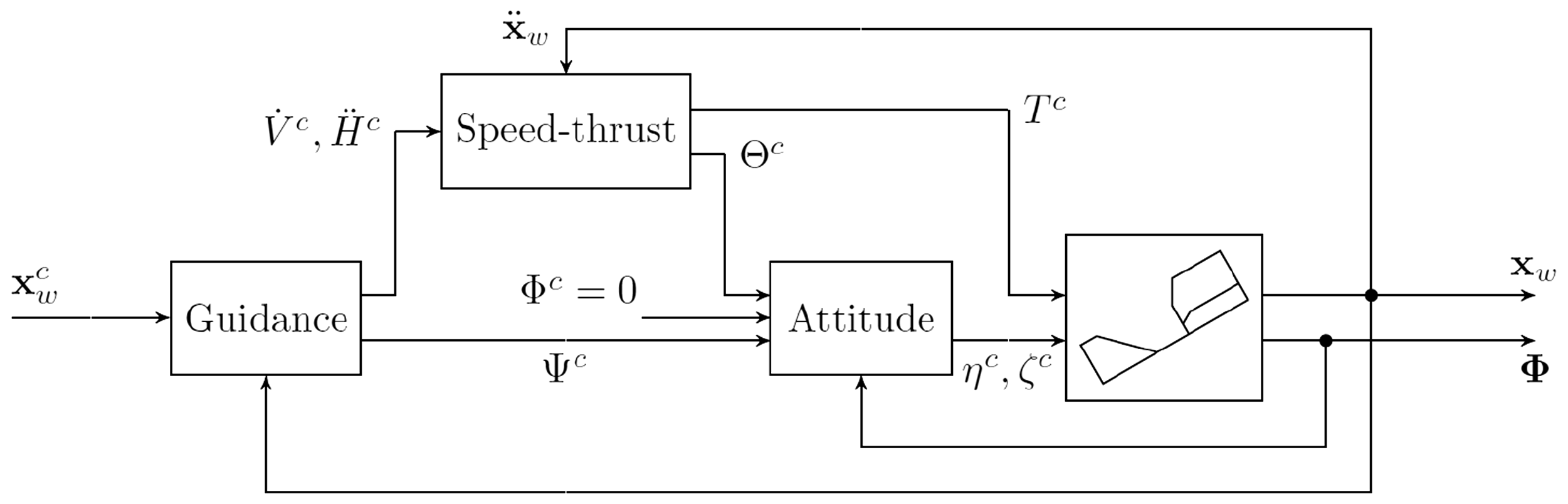
Block diagram of the cascade control approach consisting of guidance, speed-thrust and attitude controllers. Guidance block commands the desired heading $Ψ$ and accelerations ${\dot{V}}^{c}, {\ddot{H}}^{c}$ based on the current position error. The speed-thrust block determines the combination of pitch $Θ^{c}$ and thrust T^c commands that leads, at the wind tunnel speed V_W, to the desired accelerations. The attitude block controls the attitude through the rudder and elevator commands, η^c and ζ^c, respectively.

Guidance control

The guidance control is decentralised, i.e. we control the forward position x_w, height $H = - z_{w}$ and lateral position y_w in separate loops. In the longitudinal loops (forward + vertical), we assume the DelFly is always aligned with the wind tunnel axis, i.e. it is flying opposite to the wind direction ${\vec{V}}_{W}$ . Ordinary PD controllers are used in the longitudinal and vertical loops to determine the desired accelerations ${\dot{V}}^{c}$ and ${\ddot{H}}^{c}$ , which are commanded to the inner loops. Since the DelFly has no roll control authority, the lateral position y_w is controlled through heading $Ψ^{c}$ . To compensate for steady-state errors, an integral gain was introduced to the lateral loop.

The accelerations and heading commanded to the inner loops are thus determined as

{\dot{V}}^{c} = k_{dx} Δ {\dot{x}}_{w} + k_{px} Δ x_{w}

(1)

{\ddot{H}}^{c} = - k_{dz} Δ {\dot{z}}_{w} - k_{pz} Δ z_{w}

(2)

Ψ^{c} = k_{dy} Δ {\dot{y}}_{w} + k_{py} Δ y_{w} + k_{iy} \int Δ y_{w} d t

(3)

where k_p, k_d and k_i denotes the P, D and I gains, respectively, and Δ stands for the position error from the set-point.

The P and D gains of the longitudinal and vertical loops were selected based on the desired closed loop behaviour (assuming the plant to be a second-order system with no inherent damping). The gains of the lateral loop were tuned during the flight tests. All the gain values used in the presented experiments are summarised in Table 2.

Speed-thrust control

Since the generation of lift and thrust is highly coupled, a suitable combination of pitch angle Θ and throttle command T (controlling the flapping frequency f) that will result in the desired accelerations in the longitudinal and vertical directions needs to be found. This is the role of the speed-thrust control (Figure 7), which consists of a feedforward and feedback part. The feedforward control selects the necessary combination of Θ and T based on a linear model constructed from wind tunnel force measurements data. The feedback part improves the performance by correcting for model uncertainties, change of performance over time as well as external disturbances.

Figure 7.

The two-phase semi-adaptive control approach. At the start of each flight, an adaptation loop with gain γ is used to adapt the assumed equilibrium conditions T₀ and $Θ_{0}$ , until any potential position drift caused by model uncertainties of the feedforward control is removed. At time t = t_A, when the equilibrium is approached, the operator switches to the correction phase and the adapted equilibrium conditions $T_{0}^{*}$ and $Θ_{0}^{*}$ are kept. In this phase, the acceleration set-points from the outer guidance loop are tracked and an additional feedback loop is employed to compensate for disturbances, model uncertainties and performance changes due to decreasing battery voltage.

Feedforward control

Using wind tunnel data obtained with a clamped DelFly for various wind speeds V_W, pitch angles Θ and throttle commands T (the data were collected during an experiment described in Karasek et al.⁶¹), a linear relationship between the pitch angle and throttle and the measured thrust and lift forces can be found by first-order Taylor linearization

[\begin{array}{l} F_{F} \\ F_{L} \end{array}] = [\begin{array}{l} F_{F 0} (V_{W}) \\ F_{L 0} (V_{W}) \end{array}] + A (V_{W}) [\begin{array}{l} Θ - Θ_{0} (V_{W}) \\ T - T_{0} (V_{W}) \end{array}]

(4)

where

Θ_{0} (V_{W}), T_{0} (V_{W})

denote the equilibrium condition of no acceleration for wind speed V_W, resulting into a thrust

F_{F 0} (V_{W})

that is equal to drag at V_W and lift

F_{L 0} (V_{W})

that is equal to the DelFly weight.

A (V_{W})

is the matrix of force derivatives (evaluated at the equilibrium

Θ_{0} (V_{W}), T_{0} (V_{W})

)

A (V_{W}) = [\begin{array}{l} \frac{\partial F_{F}}{\partial Θ} (V_{W}) \frac{\partial F_{F}}{\partial T} (V_{W}) \\ \frac{\partial F_{L}}{\partial Θ} (V_{W}) \frac{\partial F_{F}}{\partial T} (V_{W}) \end{array}]

(5)

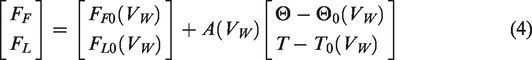
By inverting equation (4) we get

[\begin{matrix} Θ \\ T \end{matrix}] = [\begin{matrix} Θ_{0} (V_{W}) \\ T_{0} (V_{W}) \end{matrix}] + A {(V_{W})}^{- 1} [\begin{matrix} Δ F_{F} (V_{W}) \\ Δ F_{L} (V_{W}) \end{matrix}]

(6)

where

Δ F_{F} (V_{W})

and

Δ F_{L} (V_{W})

are the differences of thrust and lift from the equilibrium values

F_{F 0} (V_{W})

and

F_{L 0} (V_{W})

, respectively. Assuming the horizontal and vertical systems are decoupled and neglecting any inherent damping, the body acceleration is a result of only the forces applied,

\dot{V} = Δ F_{F} / m, \ddot{H} = Δ F_{L} / m

. Thus, the desired pitch angle and thrust can be found from the acceleration set-points as

[\begin{matrix} Θ^{c} \\ T^{c} \end{matrix}] = [\begin{matrix} Θ_{0} (V_{W}) \\ T_{0} (V_{W}) \end{matrix}] + mA {(V_{W})}^{- 1} [\begin{matrix} {\dot{V}}^{sp} \\ {\ddot{H}}^{sp} \end{matrix}]

(7)

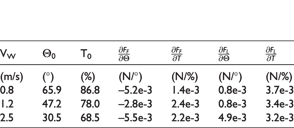
The matrix of aerodynamic force derivatives has been derived for different wind speeds, see Table 1; switching between the different values is done manually based on the wind tunnel set-point, which remains constant throughout the tests.

Table 1.

Equilibrium conditions and aerodynamic force derivatives for various wind speeds, based on wind tunnel measurements described in Karasek et al.⁶¹

V_W	$Θ_{0}$	T₀	$\frac{\partial F_{F}}{\partial Θ}$	$\frac{\partial F_{F}}{\partial T}$	$\frac{\partial F_{L}}{\partial Θ}$	$\frac{\partial F_{L}}{\partial T}$
(m/s)	(°)	(%)	(N/°)	(N/%)	(N/°)	(N/%)
0.8	65.9	86.8	–5.2e-3	1.4e-3	0.8e-3	3.7e-3
1.2	47.2	78.0	–2.8e-3	2.4e-3	0.8e-3	3.4e-3
2.5	30.5	68.5	–5.5e-3	2.2e-3	4.9e-3	3.2e-3

Table 2.

Wind speed dependent gain values of all the control loops.

	Low speed		High speed
V_W	$\approx$ 0.8 m/s	$\approx$ 1.2 m/s	$\approx$ 2 to 2.4 m/s
	Guidance control
k_px		1
k_dx		2
k_py	6	4.8	6
k_iy	0.75	0.6	0.98
k_dy	0.75	1.2	3
k_pz		1
k_dz		2
	Speed-thrust control
k_pv	0		0.3
k_iv	2		0.5
k_pf	0		1
k_if	2		0.3
γ		2.5
	Attitude control
$k_{p Θ}$	2.53		1.75
$k_{i Θ}$	0.25		0.034
$k_{d Θ}$	0.063		0.031
$k_{p Ψ}$	1.63		1.5
$k_{i Ψ}$	0.019		0
$k_{d Ψ}$	0.094		0.031
$k_{ff Ψ}$	0		5

Note: The high-speed gains are significantly different because the FWMAV gets close to the limit of inherent stability at these speeds.

Semi-adaptation

In ideal case, setting the throttle and elevator to the equilibrium values $Θ_{0} (V_{W}), T_{0} (V_{W})$ should result in steady-state flight at speed V_W. However, because the wind tunnel data used to derive the matrices of force derivatives $A (V_{W})$ were obtained with another DelFly, and because the performance of the DelFly can deteriorate over time, the DelFly will typically drift (with respect to ground). To correct for the drift, each flight started with an adaptation phase, during which the assumed equilibrium conditions $Θ_{0} (V_{W}), T_{0} (V_{W})$ are being adapted, via a position feedback, until a steady flight is reached

[\begin{matrix} Θ_{0}^{*} (V_{W}) \\ T_{0}^{*} (V_{W}) \end{matrix}] = [\begin{matrix} Θ_{0} (V_{W}) \\ T_{0} (V_{W}) \end{matrix}] + mA {(V_{W})}^{- 1} γ [\begin{matrix} Δ x_{w} \\ Δ H \end{matrix}]

(8)

where the

^{*}

superscript denotes the adapted equilibrium conditions,

Δ x_{w}

and

Δ H

are the errors from the position where the adaptation was started and γ is a positive gain. The proof that such feedback leads to a stable equilibrium is in the Appendix of Cunis et al.⁶²

Feedback control

Once the equilibrium is found, the operator switches to a correction phase, where an additional feedback loop with a PI controller is added to the feedforward control to compensate for disturbances, model uncertainties and performance changes due to decreasing battery level

[\begin{matrix} {\dot{V}}^{fb} \\ {\ddot{H}}^{fb} \end{matrix}] = [\begin{matrix} k_{pF} Δ \dot{V} \\ k_{pV} Δ \ddot{H} \end{matrix}] + [\begin{matrix} k_{iF} \int Δ \dot{V} d t \\ k_{iV} \int Δ \ddot{H} d t \end{matrix}]

(9)

The integrated error is calculated as $\int Δ \dot{V} d t = \int {\dot{V}}^{sp} d t - V, \int Δ \ddot{H} d t = \int {\ddot{H}}^{sp} d t - \dot{H}$ .

Because A contains a guess of direction of the force derivatives, we add the correction before the feedforward control. The combined control law results into

\begin{array}{l} [\begin{matrix} Θ^{c} \\ T^{c} \end{matrix}] \\ = [\begin{matrix} Θ_{0}^{*} (V_{W}) \\ T_{0}^{*} (V_{W}) \end{matrix}] + \\ + m A^{- 1} (V_{W}) ([\begin{matrix} {\dot{V}}^{sp} \\ {\ddot{H}}^{sp} \end{matrix}] + [\begin{matrix} k_{pF} Δ \dot{V} \\ k_{pV} Δ \ddot{H} \end{matrix}] + [\begin{matrix} \int k_{iF} Δ \dot{V} d t \\ \int k_{iV} Δ \ddot{H} d t \end{matrix}]) \end{array}

(10)

Attitude control

In the inner most loop, we used the Integer-quaternion implementation of the attitude stabilisation algorithm of the Paparazzi UAV system,⁵⁵ which controlled the body pitch and yaw via elevator and rudder deflections, respectively. The PID gains were tuned manually prior to the wind tunnel tests. For faster speeds, a feedforward term k_ff was used in the yaw loop. The gain values are summarised in Table 2.

PIV measurement setup and processing

High-speed Stereo-PIV measurements were performed at a spanwise-oriented plane approximately 150 mm downstream from the DelFly tail. Note that only one side of the wake was imaged, due to field of view size restrictions, however, the wake is assumed to be nominally symmetric with respect to the centre plane. The flow was illuminated with a double-pulse Nd:YLF laser (Mesa-PIV) with a wavelength of 527 nm and a pulse energy of 18 mJ (at 6 kHz). The laser sheet with a thickness of 2 mm was kept at a fixed position, while the DelFly position was varied based on the measurement case. The flow was seeded with a water–glycol-based fog of droplets with a mean diameter of 1 μm, which is produced by a SAFEX fog generator. The complete measurement room was filled with the fog beforehand in order to achieve a homogeneous seeding of the flow. Images of tracer particles were captured with two high-speed Photron FastCam CMOS cameras which allow to achieve a maximum resolution of 1024 × 1024 pixels at a data rate of up to 5.4 kHz. Each camera was equipped with a Nikon 60 mm focal objective with numerical aperture f/4 and mounted with Scheimpflug adaptors. The cameras were placed with an angle of 40° with respect to each other. A schematic overview of the PIV measurement setup can be seen in Figure 3.

A field of view of 170 mm × 170 mm was captured with a magnification factor of approximately 0.12 at a digital resolution of 6 pixels/mm. Single-frame images were recorded at a rate of 5 kHz for approximately a second, yielding a data ensemble size of about 5000 images. The associated time interval of 0.2 ms between individual frames corresponds to an out-of-plane displacement of 0.4 mm, based on the free stream velocity. This is sufficiently low with respect to the laser sheet thickness to allow for an accurate correlation of subsequent particle images. In order to increase the signal-to-noise ratio in the images, two laser cavities were shot in each single camera frame with 1 μs time delay in between, ensuring frozen particle images. The commercial software Davis 8.0 (LaVision) was used in data acquisition, image pre-processing, stereoscopic correlation of the images, and further vector post-processing. The pre-processed single-frame images were interrogated using windows of final size of 64 × 64 pixels with two refinement steps and an overlap factor of 75% resulting in approximately 4800 vectors with a spacing of 2.9 mm in each direction.

A spatio-temporal reconstruction was performed for the initial interpretation of the wake structure. For this purpose, the time-series measurements performed in the single static measurement plane (i.e. around 150 mm downstream of the DelFly tail) were employed to generate a quasi-3D representation of the wake structure by using a passive convection model (Taylorio hypothesis). This implies that the data of the measurement plane is translated with the free-stream velocity $U_{\infty} = V_{W}$ (with an assumption of non-deforming wake and neglecting the induced velocities). More precisely, from the time-resolved velocity data $u (x, y, z, t)$ recorded at the fixed streamwise position x = x₀, the volumetric representation of the instantaneous flow field at a specific time t = t₀ is computed as $u (x, y, z, t_{0}) \approx u (x_{0}, y, z, t_{0} - x / U_{\infty})$ . This approach results in a spatial resolution of 0.4–0.5 mm in the streamwise direction for the given image recording rate of 5 kHz and for the considered free-stream velocity range (2–2.4 m/s).

As a final remark, it should be mentioned that the extent to which the current representation is an accurate description of the actual spatial wake is significantly affected by the limited validity of the Taylorty hypothesis in this situation, as the true advection velocity, which is a combination of the freestream and the flow induced by the flapping wings, is far from homogeneous and varying in time over the flapping cycle.

Results

Position control

The following section shows the performance of the position control, in steady state as well as in response to a step input. During the PIV measurement, the flying DelFly should ideally stay at a prescribed constant position. Thus, our primary goal was to achieve high precision steady flight around a fixed set-point rather than fast tracking performance of a moving set-point.

Step commands

The sequence of step commands in all three wind tunnel frame axes is captured, for a wind tunnel set-point V_W = 1.2 m/s, in Figure 8. Apart from the position, we also recorded the body attitude (motion tracking system) and commands to the attitude loop and to the motor speed controller (WiFi telemetry). From the position graphs, we can see that similar rise times, between 3 and 6 s, were achieved in all the three directions. A slight overshoot and longer settling was observed especially in the lateral direction, since it was controlled indirectly, through the change of heading.

Figure 8.

Response to a sequence of step commands in all three directions at V_W = 1.2 m/s. The position set-points are displayed in black dashed lines, blue lines show the unfiltered tracking and telemetry data. The dotted vertical lines mark the time stamps of the step commands.

In longitudinal manoeuvres, it is the speed-thrust control block (Speed-thrust control section) that determines the necessary combination of throttle and elevator commands, based on current wind tunnel set-point. In Figure 8 (V_W = 1.2 m/s), the vertical manoeuvre is dominated by a throttle change, while forward manoeuvre also requires pitching the body via the elevator. Because this block is based on experimental data obtained with a slightly different aircraft, some coupling remains when forward step is commanded, nevertheless the feedback control damps these effects out. The lateral position is sensitive to both changes in vertical and forward directions, which is an inherent property of the aircraft, but again the feedback control will steer the vehicle back to the set-point through a heading change controlled by rudder deflection.

From the command plots we can further observe that the throttle command increases over time. This is due to the battery voltage, which is decreasing as the battery gets discharged, and due to the integrator action, which responds by increasing the throttle command in order to keep the flapping frequency constant. A comparison of measured body pitch with the pitch command confirms that the attitude loop manages to follow the pitch set-point. A post flight telemetry analysis showed that the decreasing trend in the yaw command is a result of a slow drift of the on-board heading estimate. While heading from the tracking system should be used for correcting the drift typical when integrating gyroscope readings, a small drift remained and was again corrected for by the integrators in the control loops. The heading measured by the tracking system remained close to zero, i.e. aligned with the wind tunnel axis.

Steady state

The results of steady flight with a fixed position set-point, performed at wind tunnel set-points V_W = 0.8 m/s, 1.2 m/s, 2.0 m/s and 2.4 m/s, are in Figure 9. Each panel shows the difference from the set-point in all three wind tunnel axes. The highlighted parts (thicker line, red colour) show the segments, where a successful PIV measurement could be performed according to our estimations, i.e. where the rms error remains below 25 mm in all three axes for the next 2 s. The rms errors over the whole measurement are summarised, together with mean body attitude angles, mean marker tracking errors and their respective standard deviations, in Table 3. All the data were measured by the motion tracking system.

Figure 9.

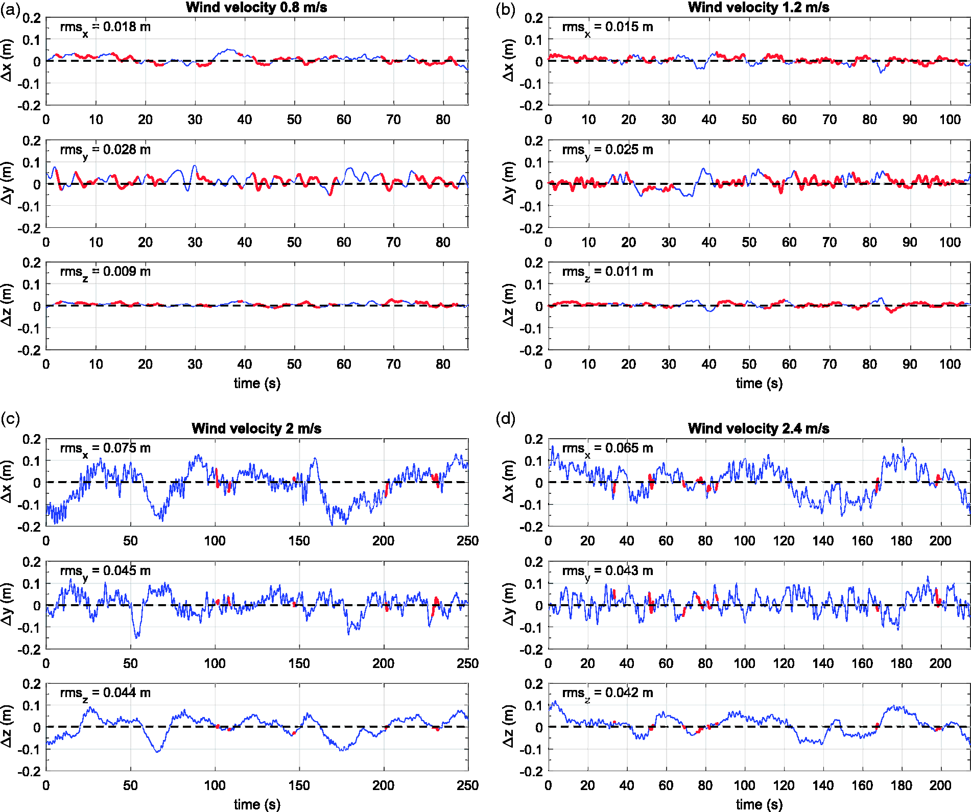
Position difference from the set-point for various wind tunnel speeds: (a) 0.8 m/s, (b) 1.2 m/s, (c) 2 m/s, (d) 2.4 m/s. Root-mean-square (rms) position error values over the whole measurement are displayed in the top left corner of each subplot. The segments where a successful PIV measurement could be performed according to our estimations (i.e. the rms error remains below 25 mm in all three axes for the next 2 s) are highlighted by a thicker red line. Significant position accuracy decrease can be observed for high speeds (2 m/s and 2.4 m/s), where the FWMAV is operated close to its inherent stability limit. Besides, the gain tuning for high speeds may not have been optimal due to time constraints during the wind-tunnel slot dedicated to the flow visualisation measurements.

Table 3.

Position precision and attitude at various wind tunnel set-points.

V_W	rms_x	rms_y	rms_z	$Φ$	Θ	$Ψ$	Track. err.
(m/s)	(mm)	(mm)	(mm)	(°)	(°)	(°)	(mm)
0.8	18	28	9	4.5 ± 3.4	68.9 ± 0.8	0.3 ± 3.4	0.73 ± 0.17
1.2	15	25	11	2.3 ± 3.1	50.5 ± 0.8	−3.1 ± 1.7	0.45 ± 0.11
2.0	75	45	44	1.5 ± 2.7	33.8 ± 1.4	−3.4 ± 1.5	0.76 ± 0.30
2.4	65	43	42	1.7 ± 2.9	28.7 ± 1.1	−3.6 ± 1.4	0.59 ± 0.19

Note: The attitude and mean marker tracking error are represented as mean ± standard deviation over the interval displayed in Figure 9.

It can be immediately noted that the performance at low speeds is much better than at high speeds. Originally, prior to the PIV test session, we tuned the controller for speeds ranging from 0.8 m/s to 1.2 m/s, where the inherent stability of the DelFly is the most pronounced. However, during the PIV session, we observed that the quality of captured data was worse than expected. The direction of the wake structures was dominated by the flapping-induced flow (aligned with the body fuselage that is pitched by 50.5° to 68.6° at slow speeds) and this resulted into a considerable angle between the measurement plane normal and the wake axis. Therefore, within the time constraints of the wind tunnel slot available for the PIV tests, we quickly tuned the controller also for high speeds (2.0 m/s and 2.4 m/s shown here), where the body pitch is much lower (33.8° to 28.7°). This was much more challenging, because the DelFly (in the configuration used for the tests) is already very hard to fly at these speeds without any stability augmentation.

At low speeds (0.8 m/s and 1.2 m/s), the position fix was very good. The best results were achieved in the vertical z_w direction, where the DelFly stayed within ±25 mm most of the time and the corresponding rms error was around 10 mm. In the forward direction, an accuracy better than ±50 mm was achieved most of the time, with an rms error of below 20 mm. Most oscillations were observed in the lateral direction, yet a large part of the time the aircraft was also within ±50 mm from the set-point, which can be seen from the rms values that remain below 30 mm. According to the estimated criteria (rms below 25 mm for the next 2 s), a successful PIV measurement could be started at 49% and 65% of the time for 0.8 m/s and 1.2 m/s, respectively, meaning that the waiting time of the operator monitoring the MAV position and triggering the PIV measurement would be very short.

At high speeds, the DelFly control is much more challenging as explained earlier. The rms error values were about 45 mm for forward and lateral directions and around 70 mm for forward direction. Despite a worse overall performance (the rms values were computed over several minutes of flight), there were segments of several seconds (highlighted parts) when the platform was very close to the set-point for at least 2 s in all the axes (3% and 4.8% of the total time for 2.0 m/s and 2.4 m/s, respectively). This gave us enough opportunities to trigger and perform successful PIV measurements also at lower body pitch angles, where the flow patterns of the wake move almost normally to the vertical measurement plane, yielding higher quality flow measurements.

The mean attitude captured at different speeds (Table 3) reveals that the roll and yaw angles were not exactly zero. This is due to imperfections of the hand-built DelFly, in particular a slight misalignment of the tail caused by a twist in the square carbon tube used as fuselage, but this has a negligible effect on the PIV measurements since the misalignment is in the order of a few degrees.

Flow visualisation

This section provides results for the first free-flight flow visualisation of the wake of the DelFly. The PIV measurements were performed in a plane oriented perpendicular to the freestream direction, at a distance of approximately 150 mm downstream of the tail, similar to measurements performed with bats of comparable sizes.³² Results are presented here for the flight condition of a freestream speed of 2.4 m/s, flapping frequency of 12.0 Hz and body angle of 28.7°. The corresponding reduced frequency, defined as $k = π fc / V_{W}$ (where f is the flapping frequency, c = 80 mm the mean wing chord and V_W the freestream velocity), has a value of 1.25. The Reynolds number is 13,000, based on freestream velocity and wing chord. For comparison, the tests were also conducted in a tethered setting with the identical DelFly, rigidly fixed according to Figure 1, similar to our previous trials.⁴⁴ The flight conditions were comparable to the free-flight tests (freestream speed of 2.0 m/s, flapping frequency of 12.1 Hz, body angle of 33.8° and Reynolds number around 11,000).

PIV images were recorded for a duration of approximately 1 s, at an acquisition frequency of 5 kHz. Given the flapping frequency of 12 Hz, this implies that 12 cycles are captured, with approximately 400 images per cycle, indicating a well-resolved characterisation of the flapping cycle. The results presented in the following are the direct outcome of the measurements, i.e. no additional averaging, smoothing or other form of filtering has been applied that could potentially further improve the quality of the visualisation.

The relative position and orientation of the FWMAV with respect to the centre of the measurement region, averaged over the duration of the PIV recording, is displayed in Figure 10. While various position set-points were tested during the trials, this relative position allowed to capture the most prominent vortex structures in the wake, originating from the right halve of the wings. The good position stability over the duration of the PIV measurement can be documented by the values of standard deviation from the mean position, which show that apart from a slight drift in the y direction ( $σ_{y} = 26.3$ mm) a very good fix was achieved both in the forward ( $σ_{x} = 5.2$ mm) and the vertical ( $σ_{z} = 4.5$ mm) axes.

Figure 10.

Relative position and orientation of the FWMAV with respect to the measurement plane (green square), averaged over the duration of the PIV measurement presented in Figures 11 and 12.

Figure 11 displays a sample time series of four images separated by 0.065 s, with the vectors indicating the in-plane velocity components and the colour contours the out-of-plane vorticity. The most prominent feature observed in the visualisations can be associated to the tip vortex of the upper wing in the instroke phase (red, corresponding to counter-clockwise vorticity).

Figure 11.

Stereo-PIV measurements in the wake of a DelFly in free-flight showing a sample sequence of four images, separated by 0.065 s, where the rightmost one is captured earliest in time; vectors indicate the in-plane velocity components and the colour contours the out-of-plane vorticity (in 1/s). Free stream velocity is 2.4 m/s; flapping frequency is 12.0 Hz.

A 3D representation of the wake vortex structure is obtained with the convection model, as described in the PIV measurement setup and processing section, which transforms the temporal information contained in the high-speed velocity field acquisition into a spatial representation by translating the flow field of subsequent images downstream with the freestream velocity. The result, displaying two flapping cycles, is shown in Figure 12. Figure 12(a) applies to the free-flight condition and Figure 12(b) to the tethered DelFly. The visualisations provide a colour coding of the helicity (density), which is defined as the scalar product of the velocity and vorticity vectors.

Figure 12.

Comparison of three-dimensional wake structure of the DelFly for (a) free-flight and (b) tethered condition; colour coding is for helicity (red: +0.6 m/s²; blue: –0.6 m/s²).

Helicity can be used for the detection of vortex cores⁶³ and non-zero helicity indicates a helical vortex structure with an axial flow. The sign of the helicity allows to distinguish vortex structures with different sense of swirl. However, it should be noted that in the current study only a portion of the actual helicity density is calculated (using the out-of-plane components of the vorticity and velocity vectors) due to planar velocity information. Despite this limitation, the helicity isosurfaces still indicate the regions of swirling motion in the wake of the flapping wings. The very prominent upper red structure (positive helicity) is the tip vortex formed by the upper wing during the instroke. The less distinct blue structure (negative helicity) is the tip vortex of the bottom wing generated during instroke as well. Structures of the outstroke appear not to be very well captured in this representation, however.

Notwithstanding the suboptimal quality of these preliminary results, an important observation is the good qualitative agreement between the free-flight and tethered wake flow structures, and the good repeatability of the two cycles for each case. This supports the conclusion that reliable and meaningful PIV measurement results have been obtained also in the free-flight case.

Conclusions and discussion

We presented a methodology, which combined an FWMAV specific control approach for autonomous flight in a wind tunnel with a time-resolved stereoscopic PIV and allowed the first flow visualisation experiments to be carried out with a freely flying flapping-wing robot. The novel FWMAV specific control approach relied on feedback from an on-board IMU and an external motion tracking system. Applied to the 25-g DelFly FWMAV, an autonomous flight with high accuracy at low speeds (0.8–1.2 m/s, maximal rms error of 28 mm over 1–2 min) and good accuracy at high speeds (2–2.4 m/s, maximal rms error of 75 mm over 3–4 min) was achieved. Moreover, even higher precision was often achieved for time intervals of several seconds. Thus, the PIV measurements, lasting around 1 s, could be triggered when the DelFly was at the ideal position, which permitted to use a smaller measurement region and resulted in high resolution flow data.

The free-flight PIV measurements were performed at high free stream speeds (2 to 2.4 m/s), where the FWMAV is pitched by 33.8° to 28.7° and flaps at frequencies of 12.1 Hz to 12.0 Hz, which corresponds to Reynolds numbers of 11,000 to 13,000 and reduced frequencies of 1.5 to 1.25. The flow was captured in a planar measurement region oriented perpendicular to the free stream direction and located in the wake approximately 150 mm downstream of the tail. For the initial interpretation of the measurements, the time-series PIV data were transformed into a quasi-3D representation of the wake structure using a passive convection model. For reference, measurements were also performed with a tethered FWMAV at comparable conditions. The first results, presented in the form of helicity isosurfaces, showed a good repeatability among flapping cycles and also qualitative agreement between the free-flight and the tethered cases, suggesting that the free-flight measurements were reliable and meaningful.

While the obtained results hold promises for future experiments with the current setup, the data quality could be further increased by certain improvements of the control approach as well as of the flow visualisation procedure itself. While our control approach was designed and tested primarily for low speeds (0.8 m/s to 1.2 m/s), the first tests revealed that the interpretation of data captured in a plane perpendicular to the free stream direction can be complicated because the relatively strong induced flow of the flapping wings, aligned with the body that is pitched by $\approx 70^{°}$ to $\approx 50^{°}$ , hits the measurement plane at considerable angles. This phenomena will diminish with increasing speed, which allowed to perform meaningful measurements at speeds of 2 m/s to 2.4 m/s. For even better results, the control approach should be revised, as the dynamics of the DelFly become much more challenging at these speeds. However, even with a further increased position accuracy, the stereoscopic PIV method limits the measurements to be conducted in the wake only, as measurements closer to or even around the wings would have to deal with laser reflections on the wings.

To enable reliable measurements around the wings, but also meaningful measurements at lower speeds, we recommend using a true 3D visualisation method such as tomographic PIV⁶⁴ for future experiments. Standard tomo-PIV using conventional seeding is not feasible, however, for the measurement volume size and data acquisition rate required for the present experimental conditions. Recent developments have explored the potential of achieving large-scale tomographic measurements by using small (sub-millimetre) neutrally buoyant helium-filled soap bubbles as tracer particles.⁶⁵ Although several studies have indeed proven the feasibility of this approach, we decided not to employ this method for the first trials because as a relatively new method it still has its own challenges, many of which are related to the soap bubbles used as seeding particles. They are being employed due to their high reflectivity, which is needed when the laser beam of finite power is expanded to illuminate larger volumes. However, the soap bubbles tend to stick to the FWMAV wing foils, which negatively affects the wing operation over time. For this reason, the exposure of the wings to the particles needs to be as limited as possible, which needs a specific measurement strategy to be used that minimises this effect.

The initial results presented here proved that the developed methodology provides a reliable and repeatable way of obtaining PIV data in free-flight and that the data quality is comparable to what is usually achieved in a (traditional) tethered setting. Moreover, this new approach, employing flying robots instead of animals, enables to perform measurements not only in steady state, but also during arbitrary controlled and reproducible manoeuvres. Although the robot will never be an exact copy of the animal, the recent research on fruit-fly-escape-manoeuvre dynamics⁶⁶ showed that flapping wing robots can bring new insights into animal flight even if they differ greatly in size and morphology. Employing flying robots mimicking the animal morphology to a greater extent would allow for flow visualisation experiments that could systematically investigate parameter changes such as wing span, aspect ratio, wing flexibility, etc., something that was not possible before in free-flight.

Footnotes

Acknowledgements

We thank Sarah Gluschitz for making the nice sketch of the experimental setup.

Declaration of conflicting interests

The author(s) declared no potential conflicts of interest with respect to the research, authorship, and/or publication of this article.

Funding

The author(s) received no financial support for the research, authorship, and/or publication of this article.

References

Keennon

Klingebiel

Won

, et al. Development of the nano hummingbird: a tailless flapping wing micro air vehicle. AIAA Paper 2012-0588, 2012, pp.1–24.

Chirarattananon

Fuller

, et al. Controlled flight of a biologically inspired, insect-scale robot. Science 2013; 340: 603–607.

Phan

Truong

Park

HC.

Implementation of initial passive stability in insect-mimicking flapping-wing micro air vehicle.

Int J Intell Unmanned Syst 2015; 3: 18–38.

Gaissert

Mugrauer

, et al. Inventing a micro aerial vehicle inspired by the mechanics of dragonfly flight. In: Natraj A, Cameron S, Melhuish C, Witkowski M (eds) Towards Autonomous Robotic Systems. TAROS 2013. Lecture Notes in Computer Science, vol. 8069. Berlin, Heidelberg: Springer Berlin Heidelberg, pp.90–100.

Roshanbin

Altartouri

Karásek

, et al. COLIBRI: a hovering flapping twin-wing robot. Int J Micro Air Vehicles 2017; 9: 270–282.

de Croon

GCHE

de Clerq

KME

Ruijsink

, et al. Design, aerodynamics, and vision-based control of the DelFly. Int J Micro Air Vehicles 2009; 1: 71–97.

De Wagter

Karasek

de Croon

Quad-thopter: tailless flapping wing robot with 4 pairs of wings. In: Moschetta

Hattenberg

de Plinval

(eds) 9th International micro air vehicles conference and competition, Toulouse, France, pp.249–256.

Ristroph

Morozova

, et al. Active and passive stabilization of body pitch in insect flight. J R Soc Interface 2013; 10: 20130237.

Muijres

Elzinga

Melis

, et al. Flies evade looming targets by executing rapid visually directed banked turns. Science 2014; 344: 172–177.

10.

Sholtis

Shelton

Hedrick

TL.

Field flight dynamics of hummingbirds during territory encroachment and defense.

Plos One 2015; 10: e0125659.

11.

Bomphrey

Nakata

Henningsson

, et al. Flight of the dragonflies and damselflies. Philos Trans R Soc Lond B Biol Sci 2016; 371: 20150389.

12.

Dickinson

Lehmann

Sane

SP.

Wing rotation and the aerodynamic basis of insect flight.

Science 1999; 284: 1954–1960.

13.

Sane

Dickinson

MH.

The aerodynamic effects of wing rotation and a revised quasi-steady model of flapping flight. J Exp Biol 2002; 205: 1087–1096.

14.

Berman

Wang

ZJ.

Energy-minimizing kinematics in hovering insect flight.

J Fluid Mech 2007; 582: 153–168.

15.

Truong

Nguyen

Truong

, et al. A modified blade element theory for estimation of forces generated by a beetle-mimicking flapping wing system. Bioinspir Biomim 2011; 6: 036008.

16.

Armanini

Caetano

de Croon

GCHE

, et al. Quasi-steady aerodynamic model of clap-and-fling flapping MAV and validation using free-flight data. Bioinspir Biomim 2016; 11: 046002.

17.

Nakata

Liu

Tanaka

, et al. Aerodynamics of a bio-inspired flexible flapping-wing micro air vehicle. Bioinspir Biomim 2011; 6: 045002.

18.

Deng

Percin

van Oudheusden

, et al. Numerical simulation of a flexible x-wing flapping-wing micro air vehicle. AIAA J 2017; 55: 2295–2306.

19.

Tay

de Baar

JHS

Percin

, et al. Numerical simulation of a flapping micro aerial vehicle through wing deformation capture. AIAA J 2018; 56: 3257–3270.

20.

Deng

Aerodynamics of flapping-wing micro-air-vehicle: an integrated experimental and numerical study. PhD Thesis, Delft University of Technology, 2016.

21.

Nakata

Liu

Aerodynamic performance of a hovering hawkmoth with flexible wings: a computational approach. Proc R Soc Lond B Biol Sci 2011; 279: 722–731.

22.

Thomas

ALR

Taylor

Srygley

, et al. Dragonfly flight: free-flight and tethered flow visualizations reveal a diverse array of unsteady lift-generating mechanisms, controlled primarily via angle of attack. J Exp Biol 2004; 207: 4299–4323.

23.

Ellington

van den Berg

Willmott

, et al. Leading-edge vortices in insect flight. Nature 1996; 384: 626–630.

24.

Willmott

Ellington

Thomas

ALR.

Flow visualization and unsteady aerodynamics in the flight of the hawkmoth, Manduca sexta.

Philos Trans R Soc Lond B Biol Sci 1997; 352: 303–316.

25.

Fuchiwaki

Kuroki

Tanaka

, et al. Dynamic behavior of the vortex ring formed on a butterfly wing. Exp Fluids 2013; 54: 1450.

26.

Henningsson

Michaelis

Nakata

, et al. The complex aerodynamic footprint of desert locusts revealed by large-volume tomographic particle image velocimetry. J R Soc Interface 2015; 12: 20150119.

27.

Warrick

Tobalske

Powers

DR.

Aerodynamics of the hovering hummingbird.

Nature 2005; 435: 1094–1097.

28.

Warrick

Tobalske

Powers

DR.

Lift production in the hovering hummingbird.

Proc R Soc B 2009; 276: 3747–3752.

29.

Altshuler

Princevac

Pan

, et al. Wake patterns of the wings and tail of hovering hummingbirds. Exp Fluids 2009; 45: 835–846.

30.

Pournazeri

Segre

Princevac

, et al. Hummingbirds generate bilateral vortex loops during hovering: evidence from flow visualization. Exp Fluids 2013; 54: 1439.

31.

Bomphrey

Taylor

Thomas

ALR.

Smoke visualization of free-flying bumblebees indicates independent leading-edge vortices on each wing pair.

Exp Fluids 2009; 46: 811–821.

32.

Hedenström

Muijres

von Busse

, et al. High-speed stereo DPIV measurement of wakes of two bat species flying freely in a wind tunnel. Exp Fluids 2009; 46: 923–932.

33.

Muijres

Christoffer Johansson

Winter

, et al. Leading edge vortices in lesser long-nosed bats occurring at slow but not fast flight speeds. Bioinspir Biomim 2014; 9: 025006.

34.

Johansson

Engel

Kelber

, et al. Multiple leading edge vortices of unexpected strength in freely flying hawkmoth. Sci Rep 2013; 3: 3264.

35.

Ortega-Jimenez

Sapir

Wolf

, et al. Into turbulent air: size-dependent effects of von Kármán vortex streets on hummingbird flight kinematics and energetics. Proc Biol Sci 2014; 281: 20140180.

36.

Berg

CVD

Ellington

CP.

The vortex wake of a ‘hovering’ model hawkmoth.

Philos Trans R Soc Lond B Biol Sci 1997; 352: 317–328.

37.

Berg

CVD

Ellington

CP.

The three-dimensional leading-edge vortex of a ‘hovering’ model hawkmoth.

Philos Trans R Soc Lond B Biol Sci 1997; 352: 329–340.

38.

Birch

Dickson

Dickinson

MH.

Force production and flow structure of the leading edge vortex on flapping wings at high and low Reynolds numbers.

J Exp Biol 2004; 207: 1063–1072.

39.

Lehmann

Sane

Dickinson

MH.

The aerodynamic effects of wing-wing interaction in flapping insect wings.

J Exp Biol 2005; 208: 3075–3092.

40.

Truong

Kim

, et al. Flow structures around a flapping wing considering ground effect. Exp Fluids 2013; 54: 1575.

41.

Cheng

Roll

Liu

, et al. Three-dimensional vortex wake structure of flapping wings in hovering flight. J R Soc Interface 2013; 11: 20130984.

42.

Zheng

Tang

A time-resolved PIV study on the force dynamics of flexible tandem wings in hovering flight.

J Fluids Struct 2016; 62: 65–85.

43.

Ren

Huang

PG.

Visualization and characterization of near-wake flow fields of a flapping-wing micro air vehicle using PIV.

J Vis 2013; 16: 75–83.

44.

Percin

van Oudheusden

Eisma

, et al. Three-dimensional vortex wake structure of a flapping-wing micro aerial vehicle in forward flight configuration. Exp Fluids 2014; 55: 1806.

45.

Deng

Percin

van Oudheusden

Experimental investigation of aerodynamics of flapping-wing micro-air-vehicle by force and flow-field measurements.

AIAA J 2016; 54: 588–602.

46.

Wiken

JN.

Analysis of a quadrotor in forward flight. Masterto Thesis, Massachusetts Institute of Technology, Cambridge, USA, 2015.

47.

Nowak

Windkanal Freiflugmessungen zur Bestimmung flugmechanischer Kenngrössen. Phd Thesis, RWTH Aachen University, Aachen, DE, 2010.

48.

Kim

Lee

Choi

, et al. Autonomous formation flight of multiple flapping-wing flying vehicles using motion capture system. Aerosp Sci Technol 2014; 39: 596–604.

49.

De Wagter

Koopmans

de Croon

GCHE

, et al. Autonomous wind tunnel free-flight of a flapping wing MAV. In: Advances in aerospace guidance, navigation and control. Berlin: Springer, 2013, pp.6033nger

50.

Caetano

Percin

van Oudheusden

, et al. Error analysis and assessment of unsteady forces acting on a flapping wing micro air vehicle: free flight versus wind-tunnel experimental methods. Bioinspir Biomim 2015; 10: 056004.

51.

de Croon

GCHE

Percin

Remes

BDW

, et al. The DelFly – design, aerodynamics, and artificial intelligence of a flapping wing robot. Netherlands: Springer, 2016.

52.

De Clercq

de Kat

Remes

BDW

, et al. Aerodynamic experiments on DelFly II: unsteady lift enhancement. Int J Micro Air Vehicles 2010; 1: 255–262.

53.

Koopmans

Tijmons

De Wagter

, et al. Passively stable flapping flight from hover to fast forward through shift in wing position. Int J Micro Air Vehicles 2015; 7: 407-418.

54.

Remes

BDW

Esden-Tempski

Van Tienen

, et al. Lisa-S 2.8g autopilot for GPS-based flight of MAVs. In: IMAV 2014: international micro air vehicle conference and competition 2014, Delft, The Netherlands, 12–15 August, 2014, pp.280014t.

55.

Paparazzi

UAV. Paparazzi UAV Wiki

, http://wiki.paparazziuav.org/wiki/Main_Page (2016, accessed 14 February 2019).

56.

Muijres

Johansson

Winter

, et al. Comparative aerodynamic performance of flapping flight in two bat species using time-resolved wake visualization. J R Soc Interface 2011; 8: 1418–1428.

57.

Henningsson

Muijres

Hedenström

Time-resolved vortex wake of a common swift flying over a range of flight speeds. J R Soc Interface 2011; 8: 807–816.

58.

Muijres

Bowlin

Johansson

, et al. Vortex wake, downwash distribution, aerodynamic performance and wingbeat kinematics in slow-flying pied flycatchers. J R Soc Interface 2012; 9: 292–303.

59.

Theys

De Vos

De Schutter

A control approach for transitioning VTOL UAVs with continuously varying transition angle and controlled by differential thrust. In: 2016 international conference on unmanned aircraft systems (ICUAS), pp.118–125. USA: IEEE.

60.

De Wagter

Dokter

de Croon

GCHE

, et al. Multi-lifting-device uav autonomous flight at any transition percentage. In: Mulder JA, Choukroun D, van Kampen E, et al. (eds) Proceedings of EuroGNC, Heidelberg: Springer Verlag, 2013, pp. 34–53.

61.

Karasek

Koopmans

Armanini

, et al. Free flight force estimation of a 23.5 g flapping wing MAV using an on-board IMU. In: The 2016 IEEE/RSJ international conference on intelligent robots and systems (IROS 2016), Daejeon, Korea, 9–14 October 2016, pp.4963. Daejon: IEEE.

62.

Cunis

Karasek

de Croon

GCHE.

Precision position control of the DelFly II flapping-wing micro air vehicle in a wind-tunnel. In: The international micro air vehicle conference and competition 2016 (IMAV 2016), Beijing, China, October 17–21, pp.1–8. Beijing: IMAV.

63.

Degani

Seginer

Levy

Graphical visualization of vortical flows by means of helicity.

AIAA J 1990; 28: 1347–1352.

64.

Scarano

Tomographic PIV: principles and practice.

Meas Sci Technol 2013; 24: 012001.

65.

Kühn

Ehrenfried

Bosbach

, et al. Large-scale tomographic particle image velocimetry using helium-filled soap bubbles. Exp Fluids 2011; 50: 929–948.

66.

Karásek

Muijres

Wagter

, et al. A tailless aerial robotic flapper reveals that flies use torque coupling in rapid banked turns. Science 2018; 361: 1089–1094.

Accurate position control of a flapping-wing robot enabling free-flight flow visualisation in a wind tunnel

Abstract

Keywords

Introduction

Methods

Experimental setup

Control

Axis system

Control overview

Guidance control

Speed-thrust control

Feedforward control

Semi-adaptation

Feedback control

Attitude control

PIV measurement setup and processing

Results

Position control

Step commands

Steady state

Flow visualisation

Conclusions and discussion

Footnotes

Acknowledgements

Declaration of conflicting interests

Funding

References