Sage Journals: Discover world-class research

Abstract

Monocular vision is increasingly used in micro air vehicles for navigation. In particular, optical flow, inspired by flying insects, is used to perceive vehicle movement with respect to the surroundings or sense changes in the environment. However, optical flow does not directly provide us the distance to an object or velocity, but the ratio of them. Thus, using optical flow in control involves nonlinearity problems which add complexity to the controller. To deal with that, we propose an algorithm that estimates distance and velocity of the vehicle based on optical flow measured from a monocular camera and the knowledge of control inputs. This algorithm applies an extended Kalman filter to state estimation and uses the estimates for landing control. We implement and test our algorithm in computer simulation and on board a Parrot AR.Drone 2.0 to demonstrate its feasibility for micro air vehicles landings. Results of the simulation and multiple flight tests show that the algorithm is able to estimate height and velocity of the micro air vehicles accurately, and achieves smooth landings with these estimates, even in windy outdoor environments.

Keywords

Distance estimation monocular vision optical flow efference copy autonomous landing

Introduction

Micro air vehicles (MAVs) have gained in popularity in recent years. Due to their small size, they are easier and safer to use than large unmanned aerial vehicles. However, the size and weight constraints make the MAVs more challenging to be deployed for autonomous missions. To deal with the problems, it requires reducing the amount of payload or sensors and developing more intelligent and efficient algorithms.

Optical flow, which can be extracted from a monocular camera, provides a very promising solution for miniaturization. Optical flow refers to the apparent visual motion of objects in a scene relative to an observer.¹ This information tells us not only how fast the camera moves, but also how close it is relative to the things it sees. Flying insects use it as the main visual cue for sensing their own movements and surrounding objects while flying. They can perform complex tasks, such as landing, by only relying on this visual input and using limited neural resources. For instance, honeybees heavily use optical flow to perceive the environment and avoid dangerous objects while flying.^2,3

To accomplish vertical landings, honeybees use a divergent pattern of optical flow or the so-called flow divergence. By keeping the flow divergence constant, honeybees can perform smooth landings. This strategy leads to exponential decay of both height and velocity to zero at touchdown, and it is ideal for MAVs landings.^4–7 Often, a straightforward proportional or proportional integral feedback controller is used for MAVs to perform constant flow divergence landing.

However, in our previous studies, we found that fixed-gain controls used in constant flow divergence can lead to instability of the landing.^8,9 This is because the critical control gain is directly proportional to the height.⁸ Most of the current approaches to solving this problem are to use a gain-scheduling technique which is actually designed according to the knowledge of an initial height.^10,11 However, if no additional sensor is installed, the height is unknown. Besides, if the initial height deviates too much from the one which is used to design the gain-scheduling structure, this method will not work properly. Thus, the knowledge of the height is important for optical flow control.

In fact, optical flow does not give us the absolute distance to a surface or velocity of the camera directly. There are four known methods to estimate distances from optical flow. First, one can add sensors that directly or indirectly measure distance, velocity, or accelerations. The right type of filtering and fusion can then give distance estimates. For instance, some studies include an inertial measurement unit (IMU), a camera sensor, and a pressure sensor, and use a Kalman-based sensor fusion technique to estimate distances.^12,13

Second, when performing a perfect constant flow divergence landing, the control input (the thrust) or so-called efference copy follows a specific monotonously decreasing function over time, which can be used to estimate distances.¹⁴ They demonstrated this approach by moving a camera along a track toward an image scene to first estimate an initial distance. Since the constant flow divergence control will result in an exponential decay of distances, they simplified the estimation problem to an exponential propagation of distances after obtaining the initial value.

Third, a stability approach that detects self-induced oscillation caused by high controller gains and uses these gains to estimate distances was introduced.⁸ He showed analytically that there exists a directly proportional relationship between the critical control gain, i.e., the gain which causes instability, and the height. Based on this relationship, the MAV detects self-induced oscillation and uses these gains to estimate the height.

Fourth, by knowing the effect of the control inputs, one can “scale” the optical flow to obtain the distance and velocity. An early study on the dynamic effects in visual servoing showed that the control gain is a function of the distance.¹⁵ It was used in an adaptive control scheme for visual servoing.¹⁶ The relationship also implies that the closed-loop response depends on the distance which opens up the possibility of estimating the distance to a target from closed-loop dynamics.

In this paper, we build upon the principle presented in the fourth method to estimate the height (distance to the ground) and vertical velocity of an MAV. An extended Kalman filter (EKF) is used to estimate the height and vertical velocity of an MAV using the knowledge of the control input in combination with the flow divergence observed from a monocular camera. This algorithm uses the efference copy to predict the effects of an action and the observed flow divergence to correct the prediction. The significant advantage of this method is that we simplify the nonlinear control of the constant flow divergence to a linear control that uses height and velocity estimates. Thus, this provides the possibility of using some optimization techniques with vision output from a monocular camera to improve the performance of the control.

The remainder of the paper is set up as follows: In the first section, we provide some knowledge about the flow divergence and the constant flow divergence guidance and control strategy. The following section describes the proposed EKF-based height and velocity estimation using the flow divergence and the control inputs, the nonlinear observability analysis of the system, and vision algorithms used to estimate flow divergence with a monocular camera. Then, the next section shows the results of estimation in computer simulation while in the succeeding section we also show the results of multiple landings of an MAV. Finally, a conclusion with future work is drawn.

Background

Flow divergence

For vertical landing of an MAV, flow divergence (D) or visual looming as shown in Figure 1 can be computed as the ratio of its vertical velocity V_Z to the height from the ground Z

D = \frac{V_{Z}}{Z}

(1)

Figure 1.

Divergence of optical flow vectors (flow divergence) when the observer is approaching a surface.

When the MAV is approaching the ground, we measure positive Z, negative V_Z, and thus D < 0 according to the coordinate systems shown in Figure 2. The camera coordinate system is assumed to coincide with the body coordinate system.

Figure 2.

MAV body (x^b, y^b, z^b) and world (x^w, y^w, z^w) coordinate systems. MAV: micro air vehicle.

Constant flow divergence guidance and control

Constant flow divergence approach has been used for vertical landing of the MAVs. This approach controls the vertical dynamics of the MAVs by tracking a constant flow divergence. When |D| equals a positive constant c, we can derive from equation (1) the height $Z = Z_{0} e - ct$ , and velocity $V_{Z} = - {cZ}_{0} e - ct$ , where Z₀ is the initial height. This shows that both height and velocity will decrease exponentially and eventually become zero when touching the ground.

A proportional feedback controller is used to track the desired flow divergence $D *$ as shown in equation (2)

μ = K_{p} (D * - D)

(2)

where K_p is the gain of the proportional controller.

A double integrator system is used to model the dynamics of an MAV toward the ground in one-dimensional space. The continuous state space model can be written as

r . (t) = f (r (t), μ (t)) = A \cdot r (t) + B \cdot μ (t) = [0100] r (t) + [01] μ (t)

(3)

y (t) = h (r (t)) = [r_{2} (t) / r_{1} (t)] = D

(4)

where

r = [r_{1}, r_{2}] T = [Z, V_{Z}] T

and μ is the control input.

It is clear that the model dynamics in equation (3) are linear but the observation in equation (4) is nonlinear. Figure 3 shows a time response of the system when tracking a constant flow divergence. In this figure, we can see that the MAV accelerates in the first 2.5 s and then decelerates to zero velocity to touch the ground. Both height and velocity of the MAV decrease exponentially to zero in the end.

Figure 3.

Height Z, velocity V_Z, and flow divergence D of an MAV during landing using constant flow divergence strategy (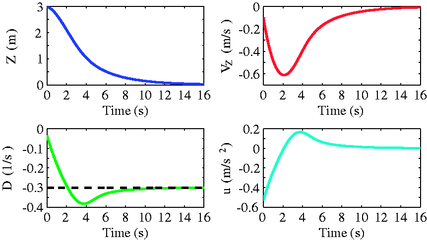 $D * = - 0.3 s - 1$ ) with control input μ. MAV: micro air vehicle.

EKF-based height and velocity estimation using flow divergence and control input

An overview of the methodology is presented in Figure 4. Images captured by a camera are served as the inputs to the software while the control input commands the actuator to control the MAV. In this section, we describe (1) an EKF algorithm using the flow divergence and efference copies to estimate the height and velocity of an MAV during landing, (2) a nonlinear observability analysis of the system, and (3) a vision method to compute the flow divergence.

Figure 4.

An overview of the methodology.

EKF

In practice, the flow divergence is computed using an on-board processor. Therefore, we used a discrete-time EKF to estimate the height and vertical velocity of the MAV. The system model and observation model are shown in equations (5) and (6), respectively

x . (t) = f (x (t), μ (t)) + w (t)

(5)

z_{k} = h (x_{k}) + v_{k}

(6)

where

f (\cdot)

and

h (\cdot)

are the system matrix and the observation matrix which are obtained from equations (3) and (4), respectively.

w (t)

and

v_{k}

are the system noise and observation noise which are both assumed to be zero mean multivariate Gaussian process with covariance Q and R, respectively.

Several computational steps taken in EKF when the update of flow divergence is obtained are shown below:

One-step ahead prediction

{\hat{x}}_{k | k - 1} = {\hat{x}}_{k - 1 | k - 1} + \int t_{k - 1} t_{k} f (x (τ), μ (τ)) d τ

(7)

Covariance matrix of the state prediction error vector

P_{k | k - 1} = Φ_{k} P_{k - 1 | k - 1} Φ_{k}^{T} + Γ_{k} Q Γ_{k}^{T}

(8)

where

Φ

and

Γ

are the discretized matrices of A and B and can be computed as below (their derivations can be found in Appendix 1)

Φ_{k} = [1 t_{k} - t_{k - 1} 01], Γ_{k} = [(t_{k} - t_{k - 1}) 2 / 2 t_{k} - t_{k - 1}]

(9)

Kalman gain

K_{k} = P_{k | k - 1} H_{k}^{⊤} (H_{k} P_{k | k - 1} H_{k}^{⊤} + R) - 1

(10)

where

H_{k} = \frac{\partial h}{\partial x} |_{{\hat{x}}_{k | k - 1}} = [- \frac{{\hat{x}}_{2_{k | k - 1}}}{{\hat{x}}_{1_{k | k - 1}}^{2}}, \frac{1}{{\hat{x}}_{1_{k | k - 1}}}] T

(11)

Measurement update

{\hat{x}}_{k | k} = {\hat{x}}_{k | k - 1} + K_{k} (z_{k} - h ({\hat{x}}_{k | k - 1}))

(12)

where

z_{k} - h ({\hat{x}}_{k | k - 1})

is called the innovation of EKF.

Covariance matrix of state estimation error vector

P_{k | k} = (I - K_{k} H_{k}) P_{k | k - 1} (I - K_{k} H_{k}) T + K_{k} R K_{k}^{T}

(13)

Nonlinear observability of the estimation

In this subsection, we show that with the flow divergence and the efference copy/control input the system is observable, i.e., any distinct states are distinguishable by applying a bounded measurable input (e.g., a piecewise constant input). To check the observability of the nonlinear system, the observability rank condition can be used.¹⁷

We first construct the observability algebra which consists of repeated Lie derivatives of the observation model in equation (4), $h (r (t)) = r_{2} (t) / r_{1} (t)$ , with respect to the model dynamics in equation (3), $f (r (t), μ (t)) = [r_{2} (t), μ] T$ . The system is observable if and only if the Jacobian of the observability algebra is full rank. In our case, the observability algebra $O$ can be written as

O = [L_{f}^{0} h (r (t)) L_{f}^{1} h (r (t))] = [h (r (t)) \frac{\partial h (r (t))}{\partial r (t)} \cdot f (r (t), μ (t))] = [r_{2} (t) / r_{1} (t) - (r_{2} (t)) 2 / (r_{1} (t)) 2 + μ / (r_{1} (t))]

(14)

Next, we analyze $O$ to see whether its Jacobian is full rank. The first function of the observability algebra is $y (t) = h (r (t)) = [r_{2} (t) / r_{1} (t)] = D$ from equation (4) while its second function is the first Lie derivative with respect to the dynamics which equals to $- (r_{2} (t)) 2 / (r_{1} (t)) 2 + μ / (r_{1} (t)) = - (h (r (t))) 2 + μ / (r_{1} (t))$ . From this result, we can clearly see that the system is (locally) observable (i.e., a full rank Jacobian of $O$ ) if and only if the control input, μ≠ 0, and $r_{1} (t) \neq 0$ and $r_{2} (t) \neq 0$ . In other words, we are able to estimate the distinct states, i.e., Z and V_Z, by using both flow divergence and control input in the algorithm.

Features-based flow divergence estimation

In computer simulation, we used equation (1) to compute flow divergence, while in flight tests, we estimated flow divergence based on equation (15) (Proof can be found in Ho et al.⁹). For each image captured by an on-board camera, corners were detected using the FAST algorithm^18,19 and tracked in the next image using the Lucas–Kanade tracker.²⁰ Then, the image distances between every two corners at one image, $d_{(t - Δ t), i}$ and at the next image, $d_{t, i}$ were computed. By further computing the ratio of $d_{(t - Δ t), i} - d_{t, i}$ to $d_{(t - Δ t), i}$ , we can measure the expansion and contraction of the flow. We took the average of these ratios, and with a known time interval between these two images $Δ t$ , we estimated divergence using equation (15)

\hat{D} = \frac{1}{n} \cdot \frac{1}{Δ t} \sum_{i = 1}^{n} [\frac{d_{(t - Δ t), i} - d_{t, i}}{d_{(t - Δ t), i}}]

(15)

where n is the total number of tracked corners. In practice, the vision output is often noisy. Therefore, we used a low pass filter to reduce the noise in the estimation.

Computer simulation

Before performing flight tests, we simulated the proposed algorithm presented in the previous section in MATLAB to show the feasibility of the algorithm.

Landing simulation with simulated control inputs

In the simulation, we generated the height and velocity with a timestamp of 0.05 s using a set of control inputs, μ as shown in Figure 5(e). These data served as ground truth for validation. The flow divergence measurement was generated using equation (1) with a measurement noise standard deviation of 0.001 s⁻¹ as illustrated in Figure 5(d).

Figure 5.

EKF-based height and vertical velocity estimation from flow divergence for landing control. (a) Height, (b) velocity, (c) innovation, (d) flow divergence, and (e) control input. EKF: extended Kalman filter.

By using the control input, μ and the flow divergence measurement, D, we estimated the height, Z and the velocity, V_Z with the proposed EKF algorithm. Figure 5 shows estimated states (Z and V_Z) and their ground truth, innovation of the EKF, flow divergence measurement, and the control inputs. In this simulation, we can observe that the estimated height and velocity converge and follow the ground truth after a few seconds, even with different initial conditions (Z₀ and $V_{Z_{0}}$ ) than the actual values. In addition, the innovation of EKF has zero mean implying that the filter is working correctly. Simulation results show that the proposed algorithm is able to estimate the distance to the ground and velocity accurately.

Experiments results and discussion

We implemented the EKF algorithm and vision algorithms in Paparazzi Autopilot, an open source autopilot software.²¹ A Parrot AR.Drone 2.0 equipped with a downward-looking camera was used as a testing platform, and all algorithms were running on board the MAV. We used an OptiTrack system to track the position of the MAV in order to provide the ground truth of its height and velocity only for validation purposes, and these measurements were not used in the estimation. In this section, we show the feasibility of the algorithm by performing three different control strategies for MAVs landings.

Before executing the algorithm in real-world experiments, we need to check the relationship between the control input μ (which is assumed to be the acceleration in the model) and the resulting acceleration a_Z imposed on our platform, e.g., $a_{Z} = f (μ)$ . Figure 6 shows the vertical acceleration a_Z resulted from the control input μ used in performing a constant flow divergence landing. The acceleration measurement was obtained from the on-board IMU but was not used in the following flight tests. Knowing that the variation of the control input μ from the hovering command μ_g is small (total command to motors $μ_{T} = μ_{g} + μ$ ), a linear function is used to map the control input to the acceleration. From the mapping, we obtained $a_{z} = 9.906 μ + 0.047$ plotted as a dashed line in the figure.

Figure 6.

Mapping of the control input μ to the vertical acceleration a_Z using a linear function ( $a_{z} = 9.906 μ + 0.047$ ).

Landing using constant flow divergence with fixed-gain control

The first strategy we used in the flight tests is the constant flow divergence. A flow divergence set point was tracked for the entire landing. During the landing, the EKF algorithm was running in real time to estimate the height and velocity of the MAV.

Figure 7 shows the estimation results of the landing with a constant divergence of $- 0.3 s - 1$ using a fixed-gain control. The initial value of the height for EKF was set to be ${\hat{Z}}_{0} = 3 m$ which was different from the true initial height, i.e., $Z_{0} \approx 2 m$ . In the figure, we can see that the height estimate converges to the true height, even though the initial value is different. In addition, the velocity estimate also matches well with the true velocity.

Figure 7.

Landing with constant flow divergence (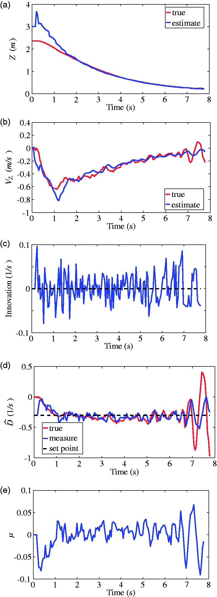 $D * = - 0.3 s - 1$ ) with EKF-based height and velocity estimation. (a) Height, (b) velocity, (c) innovation, (d) flow divergence, and (e) control input. EKF: extended Kalman filter.

From the landing results, we can observe that this strategy exponentially decreases both height and velocity to nearly zero by only tracking a constant flow divergence. In fact, the drawback of vision algorithms is that when the image is too dark, the algorithms will not work properly. For instance, when the camera is too close to the ground, the flow divergence estimate becomes incorrect. To deal with that, we constantly decrease the trim throttle when the MAV is very close to the ground ( $Z < 0.2 m$ ) to allow the MAV for touchdown. Another fact is that a fine-tuned control gain or gains adapted with the height is needed to solve the instability issue.⁹ This issue can be seen from the measured flow divergence in Figure 7(d) when the MAV is close to the ground.

To show the reliability of the proposed algorithm, we performed multiple landings with different flow divergence set points ( $D * = - 0.1, - 0.2, - 0.3 s - 1$ ) at different initial heights ( $Z_{0} \approx 2, 3 m$ ). The same initial guess of the height (3 m) was used in the EKF algorithm for these flight tests. Figure 8 shows the height and velocity estimates using EKF algorithm in different landings. In this figure, we can see that both height and velocity estimates match well with the true values. With a larger set point, the MAV landed faster with the exponential decrease in both height and velocity. Besides, these results also show that a good guess of the initial height has a faster convergence of the estimates.

Figure 8.

Multiple landings with different flow divergence set points ( $D * = - 0.1, - 0.2, - 0.3 s - 1$ ) at different initial heights ( $Z_{0} = 2, 3 m$ ). The estimates are shown with blue lines while their true values are represented by red lines.

The height and velocity estimated from EKF can then be adapted to tune the controller gain in real time for the constant divergence landing. This will be discussed in the coming section. By doing that, oscillations due to improperly chosen gain can be reduced, and thus a smooth landing can be achieved by only using a monocular camera.

Landing using constant flow divergence with height-adapted control

Experiments presented in the previous subsection were performed using a manually tuned control gain in order to achieve stable landings. In fact, the critical control gain, i.e., the control gain which causes instability, is directly proportional to the height.⁸ This means that if a fixed gain is used in constant flow divergence landing, oscillation will occur at a certain height. When the height is known from the proposed algorithm, it can be used to automatically adjust the control gain in such a way that the oscillation is eliminated.⁹ This second strategy is used to keep the advantages of using constant flow divergence landing, i.e., achieving an exponential landing profile by just tracking a desired flow divergence set point and avoid the instability due to a fixed-gain control.

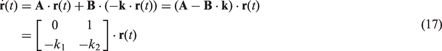
By letting $K_{p} = f (Z) = k \cdot Z$ where k is a positive constant, the proportional controller in equation (2), $μ = K_{p} (D * - D)$ becomes

μ = k \cdot Z (D * - \frac{V_{Z}}{Z}) = kD * Z - {kV}_{Z} = - k \cdot r (t)

(16)

where

k = [k_{1} k_{2}] = [- kD * k]

This controller simplifies the problem to a linear control problem. To find k, we can first solve this linear control problem using the pole-zero analysis. From equation (3), the model dynamics becomes

r . (t) = A \cdot r (t) + B \cdot (- k \cdot r (t)) = (A - B \cdot k) \cdot r (t) = [01 - k_{1} - k_{2}] \cdot r (t)

(17)

To achieve stable conditions, all the poles should lie in the left half of the s-plane. The poles of the system are obtained as shown below

λ_{1, 2} = \frac{- k_{2} \pm \sqrt{k_{2}^{2} - 4 k_{1}}}{2}

(18)

Therefore, for a stable system, $k_{2}^{2} \geq 4 k_{1}$ . By substituting $k_{1} = - kD *$ and $k_{2} = k$ , we get $k 2 \geq - 4 kD *$ and thus $k (k - 4 c) \geq 0$ , where $c = - D *$ . Since k > 0, $k \geq 4 c$ .

Three flight tests were performed at different flow divergence set points ( $D * = - 0.1, - 0.2, - 0.3 s - 1$ ) shown in Figure 9. The initial guess of the height for EKF was set to be different from the true height in order to test the convergence of the estimates. When the landing was activated, the control gain was adapted to the height according to $K_{p} = k \cdot \hat{Z}$ . Note that the value of K_p used in the real flight needs to be mapped according to the result shown in Figure 6. Since the initial height was selected to be much higher than the true height, it was expected that a slight oscillation occurred at the beginning of the landing. After the height estimate converged to the actual height, the landing was smooth as the correct gain was used. In addition, it can be seen from the last column of Figure 9 that the tracking of these three different $D *$ is good. This strategy ensures a stable and high-performance landing.

Figure 9.

Height-adapted control for constant flow divergence landings with different flow divergence set points ( $D * = - 0.1, - 0.2, - 0.3 s - 1$ ).

Landing using height and velocity from EKF

The third strategy we used for landing is tracking a height profile using the estimates from EKF. To this end, the landing begins by (1) giving an initial excitation to the MAV, or (2) using constant divergence strategy, for the first few seconds. This can ensure that the EKF converges and the controller tracks the right height estimate.

This first initialization was performed in an indoor flight test by giving a block input as the excitation as shown in Figure 10(e) to the MAV for the first 0.5 s. This allowed the MAV to go down or move in order to “observe” flow divergence and initialize the EKF algorithm. After that, the controller used the estimates from the EKF to track a desired profile or set points for landing.

Figure 10.

Landing with a linear controller using estimates from EKF (indoor flight). (a) Height, (b) velocity, (c) innovation, (d) flow divergence, and (e) control input. EKF: extended Kalman filter.

Figure 10 shows the height and velocity estimates from EKF compared with their ground truth, the innovation of EKF, the flow divergence from the vision algorithms and the ground truth, and the control input. After giving the initial excitation, the MAV started to track a height profile represented by the black dash-dot line. This profile was generated using $x_{1, k}^{*} = x_{1, k - 1}^{*} + x_{2}^{*} \cdot Δ t$ with $x_{1, 0}^{*} = {\hat{Z}}_{0}$ and $x_{2}^{*} = - 0.2 m s - 1$ . The results show that the height and velocity can be estimated accurately using the proposed EKF algorithm and further used in the controller for landing. The zero mean innovation of the EKF also tells us that the filter was working properly.

The second initialization was conducted in an outdoor flight by tracking a desired divergence for the first few seconds as shown in Figure 11. Since the OptiTrack system is not available for outdoor flight, we can only use the onboard sensor, such as sonar, to provide the true height and velocity (dZ/dt) for accuracy comparison.

Figure 11.

Landing with a linear controller using estimates from EKF (outdoor flight). (a) Height, (b) velocity, (c) innovation, (d) flow divergence, and (e) control input. EKF: extended Kalman filter.

The landing started at 5 m, and the desired divergence of $- 0.2 s - 1$ was tracked. After 2 s, the controller was switched to track a height profile as presented in Figure 11(a) which was generated based on the velocity estimate at the instance when the controller was switched ( $\approx - 0.8 m s - 1$ ). In fact, the height profile can also be created based on the desired velocity (see Figure 10). The results show that both height and velocity estimates are accurately estimated compared to the measurements from sonar. In addition, the height estimate can also be used in landing control. It can also be observed from Figure 11 that the estimates converge soon after the landing starts. Thus, the time interval for initialization can also be shortened. Note that the previous indoor flights were performed to validate the proposed algorithm using the highly accurate OptiTrack system while the outdoor flight was conducted to show the robustness of the algorithm to a windy outdoor environment. Some videos of the flight tests are available online.^a

In this paper, we presented three landing strategies using (1) constant flow divergence with fixed-gain control, (2) constant flow divergence with height-adapted control, and (3) height and velocity estimates. All these strategies can provide a smooth landing solution for MAVs. The first strategy, however, requires a perfectly tuned control gain to avoid instability. The second strategy solves this manual tuning problem by adapting height estimate from EKF to the control gain. This allows stable landings without affecting the tracking performance. Due to fast convergence of height, we only observe a slight oscillation at the start of the landings. Lastly, the third strategy uses the height and velocity from EKF directly for landing. Although it requires an initial excitation for observing optical flow, this strategy lands the MAV by following a desired landing profile and allows further performance improvement using gain optimization techniques.

Discussion on wind effect and rejection

In principle, external disturbance, such as the wind, has no problem in control as it can be rejected easily. For instance, when using a proportional feedback control with height estimates, the steady-state error due to wind can occur, but it can be eliminated using the analysis of final value theorem on our model with the wind. From this analysis, we found that in order to reject for instance a constant wind, the proportional control gain should be $K_{P} = d_{0} / x (\infty)$ , where $x (\infty)$ is the required steady-state error, and d₀ is the wind disturbance estimate.

However, for state estimation, the wind as the external force is not accounted for in our model at the moment. The practical experiment performed in a windy outdoor environment shows that this factor might not be problematic. However, a more thorough investigation and a solution for this problem might be necessary. For instance, we can augment the state vector in equation (3) with the wind disturbance as an additional state, i.e., ${\overset{\cdot}{d}}_{wind} = w$ (w can be modeled by the random walk^22,23) and modify the second state to be $V_{Z} . = μ + d_{wind}$ . By doing that, the wind factor is included in the model, and thus the estimation can be improved in the presence of the wind.²⁴ Both discussions to deal with external disturbance will be the future work of this study.

Conclusion

In conclusion, we proposed an algorithm to use an EKF to estimate the height and vertical velocity of an MAV from the flow divergence and the knowledge of the control input while approaching a surface and use these estimates for landing control. This algorithm was tested in computer simulation as well as in multiple flight tests in indoor and windy outdoor environments. The results show that the proposed EKF approach managed to estimate the height and velocity of the MAV accurately compared to the ground truth provided by the external cameras. In addition, the estimates were used in the controller to smoothly land the MAV. The proposed approach avoids the complexity of having nonlinearity in the constant flow divergence-based landing by “splitting” the flow divergence into the height and velocity which allows the use of a linear controller. For future work, an augmented state Kalman filter can be used to improve the estimation when strong external disturbances are involved. Also, the algorithm opens up the possibilities to use gain optimization techniques to improve the control performance.

Footnotes

Declaration of conflicting interests

The author(s) declared no potential conflicts of interest with respect to the research, authorship, and/or publication of this article.

Funding

The author(s) received no financial support for the research, authorship, and/or publication of this article.

Note

Appendix 1: Discretization of linear state space models

References

Gibson JJ (1950) The perception of the visual world. Boston: Houghton Mifflin.

Srinivasan

Zhang

Lehrer

et al.

Honeybee navigation en route to the goal: visual flight control and odometry. J Exp Biol 1996; 199: 237–244.

Tammero

Dickinson

. The influence of visual landscape on the free flight behavior of the fruit fly drosophila melanogaster. J Exp Biol 2002; 205: 327–343.

McCarthy

Barnes

Mahony

. A robust docking strategy for a mobile robot using flow field divergence. IEEE Trans Robot 2008; 24: 832–842.

Herisse B, Russotto FX, Hamel T, et al. Hovering flight and vertical landing control of a VTOL unmanned aerial vehicle using optical flow. In: IEEE/RSJ international conference on intelligent robots and systems, 2008. IROS 2008, Nice, France, 2008, pp.801–806. IEEE.

Ruffier F and Franceschini N. Aerial robot piloted in steep relief by optic flow sensors. In: IEEE/RSJ international conference on intelligent robots and systems, 2008. IROS 2008. IEEE, 2008, pp.1266–1273.

Alkowatly

Becerra

Holderbaum

. Bioinspired autonomous visual vertical control of a quadrotor unmanned aerial vehicle. J Guid Control Dyn 2014, pp. 38: 249–262.

de Croon

GCHE

. Monocular distance estimation with optical flow maneuvers and efference copies: a stability-based strategy. Bioinspir Biomimet 2016; 11: 016004.

Ho HW, de Croon GCHE, van Kampen EJ, et al. Adaptive control strategy for constant optical flow divergence landing. ArXiv preprint arXiv:1609.06767, 2016.

10.

Kendoul

. Four-dimensional guidance and control of movement using time-to-contact: application to automated docking and landing of unmanned rotorcraft systems. Int J Robot Res 2014; 33: 237–267.

11.

de Croon

GCHE

Alazard

Izzo

. Controlling spacecraft landings with constantly and exponentially decreasing time-to-contact. IEEE Trans Aerosp Electr Syst 2015; 51: 1241–1252.

12.

Lynen S, Achtelik MW, Weiss S, et al. A robust and modular multi-sensor fusion approach applied to MAV navigation. In: 2013 IEEE/RSJ international conference on intelligent robots and systems, Tokyo, Japan, 2013, pp.3923–3929. IEEE.

13.

Engel

Sturm

Cremers

. Scale-aware navigation of a low-cost quadrocopter with a monocular camera. Robot Auton Syst 2014; 62: 1646–1656.

14.

van Breugel

Morgansen

Dickinson

. Monocular distance estimation from optic flow during active landing maneuvers. Bioinspir Biomimet 2014; 9: 025002.

15.

Corke PI and Good MC. Dynamic effects in high-performance visual servoing. In: 1992 IEEE international conference on robotics and automation, 1992. Proceedings. Nice, France, 1992, pp.1838–1843. IEEE.

16.

Asl

Oriolo

Bolandi

. An adaptive scheme for image-based visual servoing of an underactuated UAV. Int J Robot Autom 2014; 29: 92–104.

17.

Hermann

Krener

. Nonlinear controllability and observability. IEEE Trans Autom Control 1977; 22: 728–740.

18.

Rosten E and Drummond T. Fusing points and lines for high performance tracking. In: Tenth IEEE international conference on computer vision, 2005. ICCV 2005, Vol. 2. Beijing, China, 2005, pp.1508–1515. IEEE.

19.

Rosten E and Drummond T. Machine learning for high-speed corner detection. In: Computer Vision–ECCV 2006, Graz, Austria, 2006, pp.430–443. Springer.

20.

Bouquet JY (2000) Pyramidal implementation of the Lucas Kanade feature tracker. Intel Corporation, Microsoft Research Labs, Tech. Rep.

21.

Remes BDW, Hensen D, van Tienen F, et al. Paparazzi: how to make a swarm of Parrot AR Drones fly autonomously based on GPS. In: International Micro Air Vehicle Conference and Flight Competition (IMAV2013), Toulouse, France, 2013, pp.17–20.

22.

Hsieh

. Robust two-stage Kalman filters for systems with unknown inputs. IEEE Trans Autom Control 2000; 45: 2374–2378.

23.

Park

Kim

Kwon

et al.

Estimation and detection of unknown inputs using optimal FIR filter. Automatica 2000; 36: 1481–1488.

24.

van Kampen

de Visser

et al.

Nonlinear aircraft sensor fault reconstruction in the presence of disturbances validated by real flight data. Control Eng Pract 2016; 49: 112–128.

25.

DeCarlo RA. Linear systems: a state variable approach with numerical implementation. Upper Saddle River, NJ, USA: Prentice-Hall, Inc, 1989.

Distance and velocity estimation using optical flow from a monocular camera

Abstract

Keywords

Introduction

Background

Flow divergence

Constant flow divergence guidance and control

EKF-based height and velocity estimation using flow divergence and control input

EKF

Nonlinear observability of the estimation

Features-based flow divergence estimation

Computer simulation

Landing simulation with simulated control inputs

Experiments results and discussion

Landing using constant flow divergence with fixed-gain control

Landing using constant flow divergence with height-adapted control

Landing using height and velocity from EKF

Discussion on wind effect and rejection

Conclusion

Footnotes

Declaration of conflicting interests

Funding

Note

Appendix 1: Discretization of linear state space models

References