Assessing thermoacoustic quality in combustion systems using the stability quality factor S

Abstract

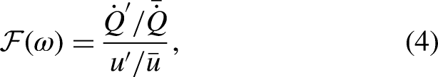
Thermoacoustic instability poses a significant challenge in the development of combustion appliances, where the lack of specific information on upstream and downstream acoustic terminations during the research and development phase is common. This knowledge gap often necessitates extensive trial-and-error approaches, emphasizing the need for a reliable indicator to assess thermoacoustic quality in advance. Traditionally, a burner and its associated flame are characterized as an acoustically active two-port block, coupled with passive acoustic terminations upstream and downstream. In this paper, we investigate the application of the direct conservative stability criterion in the frequency domain to introduce a suitable indicator, termed the $\mathcal{S}$ factor, as a figure-of-merit for thermoacoustic quality. We explore various scenarios that may arise during the research and development phase of thermoacoustically stable combustion systems. Additionally, we address the limitations associated with using Monte Carlo simulations to determine the probability of instability as a potential figure-of-merit. Our findings highlight potential misinterpretations and misrepresentations when employing the Monte Carlo approach to evaluate and compare the thermoacoustic quality of different burners and flames. Finally, the applicability of the $\mathcal{S}$ factor is demonstrated and experimentally validated in the lab-scale thermoacoustic system to rank two different burners at the same thermal power.

Introduction

The increasing need to reduce pollutants in combustion systems has led to advancements in lean premixed combustion technology. However, this method is susceptible to thermoacoustic instabilities. In the research and development (R&D) phase of combustor design, the prevalent lack of information regarding upstream and downstream acoustic terminations necessitates an extensive trial-and-error process. This underscores the critical need for a reliable indicator as “figure-of-merit” to assess the thermoacoustic quality of diverse combustors. Consequently, it becomes desirable to define the primary objective of combustor development: maximizing the range of acoustically stable operations, while simultaneously addressing crucial requirements such as minimizing emissions and pressure drop, maximizing modulation range and durability, and ensuring human health safety, among others. This study aims to introduce a novel idea of numerical metric that encapsulates one or more system characteristics, acting as a gauge of efficiency or effectiveness. This metric facilitates a meaningful comparison of thermoacoustic quality among various combustors.

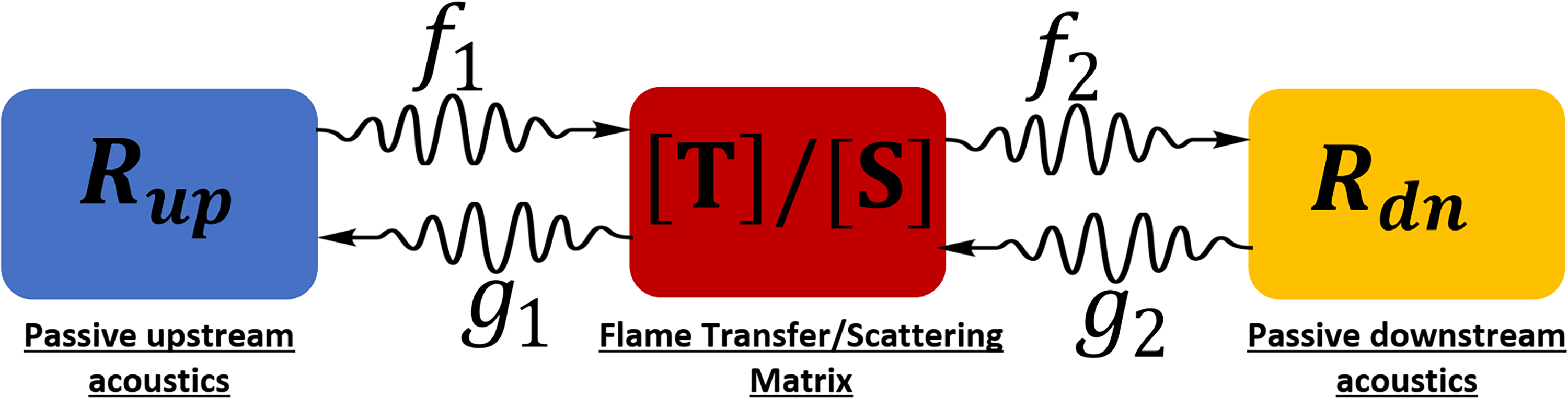
The exploration of thermoacoustic instability prediction and control has been the subject of extensive research.^1–6 Initially, there was a widespread belief in the inherent interdependence of the interaction between acoustic terminations and the burner with a flame. However, employing a “divide and conquer” strategy, such as utilizing one-dimensional network modeling, enables a more comprehensive understanding of the interplay between flame and acoustics. ⁷ In this acoustic network model, the output of each element serves as the input for the connected element, facilitating the abstract representation of a general combustion system as a network with a three-box configuration, in which one two-port network is connected to two one-port acoustic terminations, as depicted in Figure 1.

Figure 1.

Generic one-dimensional (1D) acoustic network model of a combustion system in multiple-input-multiple-output layout.

Building upon the pioneering work of Auregan and Starobinski ⁸ and subsequent advancements by Polifke et al.,^9,10 the concept of figure-of-merit in thermoacoustics based on an activity/passivity check has emerged. These formulations offer insights into the frequency range where the flame, irrespective of surrounding acoustic conditions, functions either as an acoustic energy source or sink. This concept holds promise for optimizing the performance of two-port (active) devices to achieve maximum amplification of acoustic power. ¹¹ However, it is noted that the exclusion of acoustic losses and even the requirement of passivity from the environmental representation renders this criterion ultra-conservative,^10,12 resulting in a very narrow frequency range for classifying the flame as a passive element. Furthermore, there has been a lack of direct comparison among multiple burners with their respective flames, lacking the illustration of how one can effectively compare the thermoacoustic quality of various burners.

Kornilov and de Goey ¹³ explored the application of Monte Carlo (MC) simulation to assess the stability of a burner with its corresponding flame within a system featuring randomly selected sets of frequency-independent upstream and downstream reflection coefficient values. They introduced a performance metric named the probability of instability( $\mathcal{P}\mathcal{I}$ ), calculated by determining the ratio of unstable cases in the MC simulation to the total number of cases. Subsequently, Saxena et al.^14,15 extended this MC simulation using the concept of strictly positive real (SPR) functions to generate a library of frequency-dependent reflection coefficients. However, the lack of comprehensive comparisons for different types of flames raises questions about the robustness of this method. They also developed a custom-built experimental setup that allowed for the adjustable values of upstream reflection coefficients in combination with varied downstream mufflers to perform an experimental study on a few known conditions. ¹⁴

Recently, Kornilov and de Goey ¹⁶ explored the potential of employing the MC method for randomly sampling the acoustic factor. This approach involves considering the acoustic factor as a mapping of two randomly selected passive reflection coefficients from upstream and downstream subsystems relative to the flame. In situations where the dispersion relation is factorized, this method allows for the elucidation of the universal probability density field of the acoustic subsystem factor in its complex plane. Such analysis may facilitate the assessment of the probability of burner instability.

While previous studies have suggested using the $\mathcal{P}\mathcal{I}$ obtained from MC simulations as an indicator of the thermoacoustic quality of a combustion system, this work aims to challenge that idea and demonstrate its potential pitfalls along with, this we propose an alternative approach to obtain the so-called stability quality factor ( $\mathcal{S}$ factor) that can be applied to assess the thermoacoustic quality of different burners and combustors with their corresponding flames and also ranking them based on their risk of instability. To achieve this, we employ a frequency domain analysis utilizing the direct conservative stability (DCS) criterion. By systematically considering all possible values for the passive reflection coefficients within the unit circle in a complex domain, we identify safe and unsafe regions at each frequency. This approach challenges the conventional notion of relying solely on the $\mathcal{P}\mathcal{I}$ and puts forth the stability quality factor $\mathcal{S}$ as a better alternative measure of the thermoacoustic quality of a burner.

The rest of this article is organized as follows: The next section provides a brief overview of the main features of thermoacoustic systems based on a network modeling approach. We then discuss the relevant fundamental concepts of Cauchy’s argument principle to use as a starting point to delve into some assumptions in formulating DCS criterion as the basis of the proposed stability quality factor $\mathcal{S}$ as a numerical performance metric to assess the thermoacoustic quality of known possibly active system (or subsystems). The following sections contain the main results and discussions of the paper. We showcase the effectiveness of the current stability quality factor $\mathcal{S}$ to serve as a figure-of-merit in thermoacoustics. Various burner design scenarios are explored to offer a comprehensive perspective in this context. In addition, using the DCS criterion, we highlight the potential limitations of MC simulations and the concept of $\mathcal{P}\mathcal{I}$ to be used as a thermoacoustic quality factor. Following this, the applicability of the $\mathcal{S}$ factor has been demonstrated and validated experimentally, including all necessary steps to rank two real burners. Supplemental videos accompany the figures to provide additional clarity to the concepts discussed. In the end, after a brief recap of the main concepts, conclusions are formulated.

Methodology

Network modeling and dispersion relation

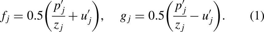
To utilize one-dimensional linear acoustic network modeling effectively, it is crucial to ensure that the frequency range of interest remains within the confines of the cutoff frequency of the first transverse mode. ¹⁷ This condition is typically applicable in the field of thermoacoustics for numerous common appliances. There are several options available for the variables used to define the acoustic two-port description, and consequently, the transfer matrices of the elements can vary accordingly. In this paper, our attention is directed toward the Riemann invariants $f_j$ and $g_j$ , which are expressed in terms of the complex acoustic pressure $p_j^{\mathrm{\prime }}$ and the acoustic particle velocity $u_j^{\mathrm{\prime }}$ , where $j=1,2$ . The indices $1$ and $2$ denote the upstream and downstream conditions, respectively. It is noteworthy that this formulation holds true, particularly in the limit of zero Mach number.

$$f_j=0.5(\frac{p_j^{\mathrm{\prime }}}{z_j}+u_j^{\mathrm{\prime }}),g_j=0.5(\frac{p_j^{\mathrm{\prime }}}{z_j}-u_j^{\mathrm{\prime }})$$

(1)

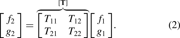
The characteristic impedance can be defined as $z_j={\rho }_{0j}{c}_{0j}$ , where ${\rho }_{0j}$ and $c_{0j}$ represent the densities and speeds of sound in the fluid, respectively. ¹⁷ It is important to note that the values of ${\rho }_{0j}$ and $c_{0j}$ differ between the upstream and downstream sides of the burner. When expressing the forward and backward traveling waves on one (physical) side of the element as a function of those on the other side, a set of interrelations is obtained. These interrelations involve a transfer matrix denoted as $\mathbf{T}$ :

$$\left[\begin{array}{c}{f}_2\\ g_2\end{array}\right]=\stackrel{[\mathbf{T}]}{\overbrace{\left[\begin{array}{cc}{T}_{11}& T_{12}\\ T_{21}& T_{22}\end{array}\right]}}\left[\begin{array}{c}{f}_1\\ g_1\end{array}\right]$$

(2)

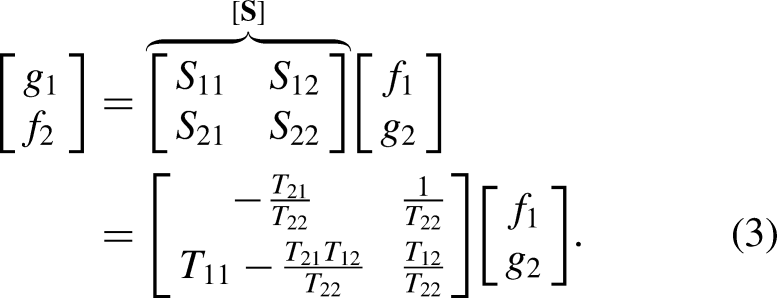
An especially insightful description can be attained by reorganizing the equations of $\mathbf{T}$ so that the ingoing waves $(f_1,g_2)$ are depicted as inputs to the matrix, while the outgoing waves $(g_1,f_2)$ are portrayed as outputs. This reconfiguration yields what is known as the scattering matrix $\mathbf{S}$ formalism:

$$\left[\begin{array}{c}{g}_1\\ f_2\end{array}\right]=\stackrel{[\mathbf{S}]}{\overbrace{\left[\begin{array}{cc}{S}_{11}& S_{12}\\ S_{21}& S_{22}\end{array}\right]}}\left[\begin{array}{c}{f}_1\\ g_2\end{array}\right]=\left[\begin{array}{cc}-\frac{T_{21}}{T_{22}}& \frac{1}{T_{22}}\\ T_{11}-\frac{T_{21}{T}_{12}}{T_{22}}& \frac{T_{12}}{T_{22}}\end{array}\right]\left[\begin{array}{c}{f}_1\\ g_2\end{array}\right]$$

(3)

The diagonal elements $S_{11}$ and $S_{22}$ signify the reflection coefficients observed from the up- and downstream sides of the element. On the other hand, $S_{21}$ and $S_{12}$ denote the transmission coefficients to the up- and downstream sides, respectively.

In the realm of thermoacoustics, a common occurrence arises when the mean and oscillatory components of the heat-release rate become localized within a region significantly smaller than the acoustic wavelength. Consequently, simplifying the conservation equations for the flame leads to the adoption of jump conditions known as Rankine–Hugoniot (R–H) relations. These relations serve to establish the connection between acoustic quantities upstream and downstream of the flame. In the case of laminar premixed flames, it is conventionally assumed that fluctuations in heat-release rate primarily originate from velocity fluctuations upstream of the flame. Thus, in such scenarios, a flame transfer function (TF) $\mathcal{F}(\omega )$ can be delineated as the normalized ratio of heat-release rate fluctuation ${\dot{Q}}^{\mathrm{\prime }}/\overline{\dot{Q}}$ to the normalized ratio of acoustic velocity excitation $u^{\mathrm{\prime }}/\overline{u}$ at a designated reference location upstream of the burner.

$$\mathcal{F}(\omega )=\frac{{\dot{Q}}^{\mathrm{\prime }}/\overline{\dot{Q}}}{u^{\mathrm{\prime }}/\overline{u}}$$

(4)

where $\overline{\dot{Q}}$ , $\overline{u}$ are the mean heat release and unburned mixture velocity, respectively. By substituting $\mathcal{F}(\omega )$ into acoustic R–H relations, the flame transfer matrix of the flame can be written as ¹⁸ :

$$T^f=\left[\begin{array}{c}{T}_{11}^f{T}_{12}^f\\ T_{21}^f{T}_{22}^f\end{array}\right]$$

(5a)

$$T_{11}^f=T_{22}^f=0.5(ϵ+1+\theta \mathcal{F})$$

(5b)

$$T_{12}^f=T_{21}^f=0.5(ϵ-1-\theta \mathcal{F})$$

(5c)

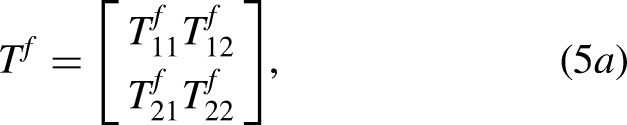
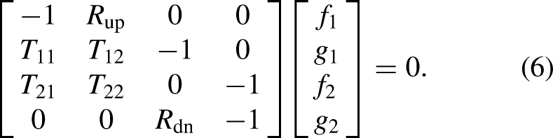
where $\theta =T_2/T_1-1$ is the temperature jump, and $ϵ={\rho }_1{c}_1/{\rho }_2{c}_2$ the specific impedance jump across the flame. If the burner is acoustically transparent, meaning it has no acoustic reflections or damping, the total transfer matrix (TM) of the active subsystem (burner with flame) is identical to the TM of the flame itself, that is, $T_{11}=T_{22}=T_{11}^f,T_{12}=T_{21}=T_{12}^f$ . In a more general case the transfer/scattering matrices of an active subsystem in Figure 1 may differ from one of the flames only. For the abstract model in terms of the scattering matrix $S$ , shown in Figure 1, the total set of system equations, is given by,

$$\left[\begin{array}{cccc}-1& R_{\mathrm{up}}& 0& 0\\ T_{11}& T_{12}& -1& 0\\ T_{21}& T_{22}& 0& -1\\ 0& 0& R_{\mathrm{dn}}& -1\end{array}\right]\left[\begin{array}{c}{f}_1\\ g_1\\ f_2\\ g_2\end{array}\right]=0$$

(6)

It is important to note that all entries of $T_{ij}$ and $R_{\text{up/dn}}$ are generally the Laplace variable ( $s=i\omega +\sigma$ )-dependent entities, considering convention of the time dependency expressed in the form of $e^{st}$ within the governing equations. The system of linear homogeneous equations possesses a nontrivial solution when the determinant of the corresponding system matrix equals zero. This determinant can be explicitly expressed as:

$${\mathrm{\Pi }}^T=T_{22}-T_{12}{R}_{\mathrm{dn}}+T_{21}{R}_{\mathrm{up}}-T_{11}{R}_{\mathrm{up}}{R}_{\mathrm{dn}}=0$$

(7)

A conventional approach involves seeking the roots of the dispersion relation, as expressed in equation (7), to derive a set of eigenfrequencies. The roots (zeros) of this equation situated within the right-half plane (RHP) of the $s$ -plane signify unstable solutions, characterized by exponential growth over time. However, it is pertinent to note that in this study, we refrain from pursuing this method.

Stability analysis in frequency domain

The precise localization of the roots (zeros) of the dispersion relation in the $s$ -plane is pivotal for resolving the dilemma of system stability–instability. To address this issue, one can leverage analysis methods developed in complex function analysis theory. This section commences with an in-depth introduction to the fundamental principles derived from complex function theory. ¹⁹ Subsequently, we delve into the practical application of these principles to analyze the stability challenge and streamline the task of stabilizing flames.

Cauchy’s argument principle ²⁰

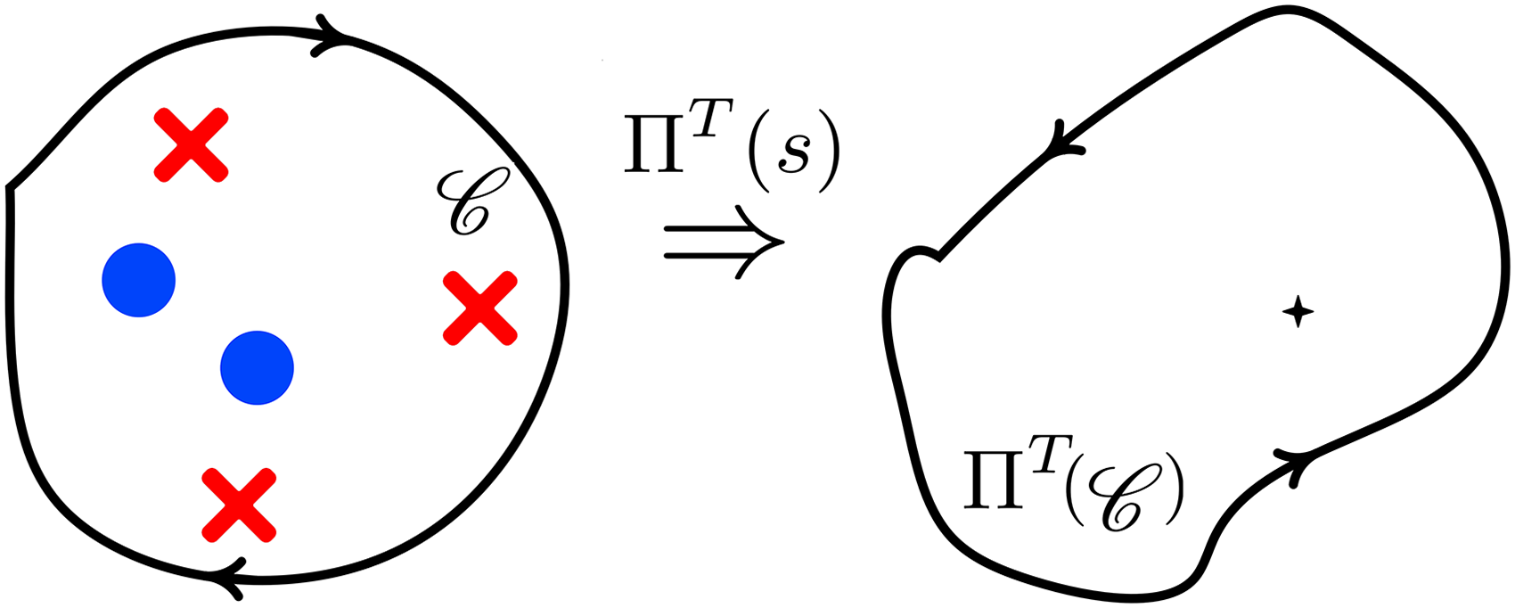
If ${\mathrm{\Pi }}^T(s)$ is a generic holomorphic and nonzero at each point of a simple closed contour $\mathcal{C}$ and is meromorphic inside $\mathcal{C}$ , then.

$$\mathcal{Z}-\mathcal{P}=\mathcal{N}=\frac{1}{2\pi i}{\oint }_{\mathcal{C}}\frac{1}{{\mathrm{\Pi }}^T(s)}\frac{d{\mathrm{\Pi }}^T(s)}{ds}ds=-\frac{1}{2\pi }\mathrm{\Xi }({\mathrm{\Pi }}^T)$$

(8)

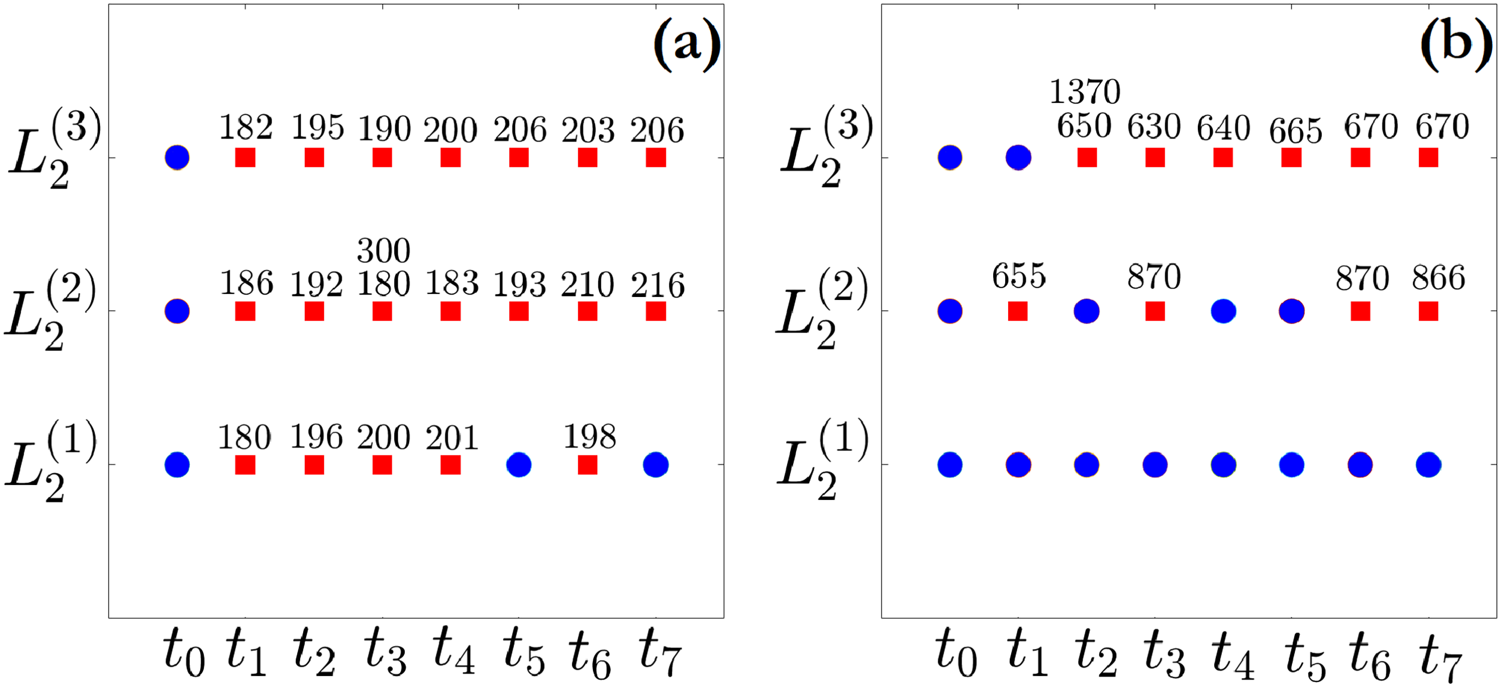
where $\mathcal{Z}$ and $\mathcal{P}$ are accordingly the number of zeros and poles of ${\mathrm{\Pi }}^T(s)$ evaluated in the domain encompassed by the contour $\mathcal{C}$ . $\mathcal{N}$ is known as the winding number of ${\mathrm{\Pi }}^T(\mathcal{C})$ , and counts the number of turns that the curve ${\mathrm{\Pi }}^T(\mathcal{C})$ winds clockwise around the origin. $\mathrm{\Xi }({\mathrm{\Pi }}^T)$ indicates the unwrapped argument of ${\mathrm{\Pi }}^T$ . Figure 2 shows a clarification example of using Cauchy’s argument principle when ${\mathrm{\Pi }}^T(s)$ is evaluated along contour $\mathcal{C}$ , in which the blue circles and the crosses in red represent zeros and poles of ${\mathrm{\Pi }}^T(s)$ , respectively. The number of encirclements can be easily calculated as $\mathcal{N}=2-3=-1$ .

Figure 2.

A clarification example of Cauchy’s argument principle. The blue circles and crosses in red represent zeros and poles of ${\mathrm{\Pi }}^T(s)$ in the $s$ -plane, respectively, and so the number of encirclements in ${\mathrm{\Pi }}^T(s)$ -plane around the origin shown with a black star can be calculated as $\mathcal{N}=2-3=-1$ .

Thermoacoustic stability analysis using Cauchy’s argument principle

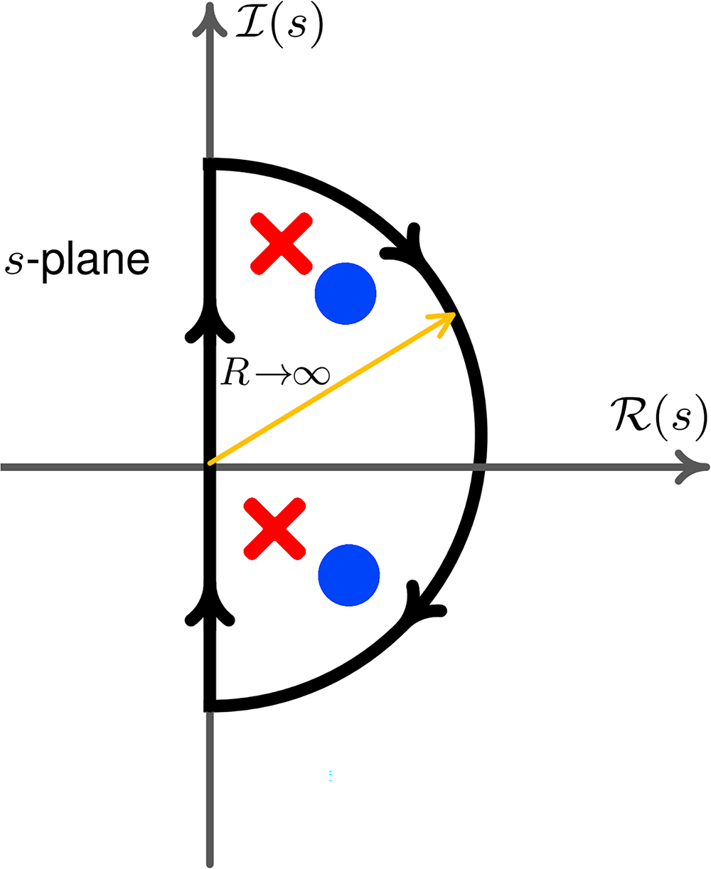
To evaluate the exponential stability of a linear thermoacoustic system, one must examine the presence or absence of RHP zeros in the dispersion relation. Utilizing Cauchy’s argument principle enables the identification of RHP zeros and poles of the characteristic function ${\mathrm{\Pi }}^T(s)$ without the necessity of explicitly solving the dispersion relation in the complex plane. This assessment is performed by applying Cauchy’s argument principle using a contour $\mathcal{C}$ that encloses the entire RHP ( $\mathcal{C}={\mathcal{D}}^{+}$ ), as depicted in Figure 3. Consequently, knowledge of the function ${\mathrm{\Pi }}^T(s)$ along the imaginary axis and at infinity is required. In many physical systems, the frequency response ${\mathrm{\Pi }}^T(i\omega )$ proves sufficient for stability assessment, particularly when evaluating a (semi-)proper target function with the property $\underset{s\to +\mathrm{\infty }}{lim}{\mathrm{\Pi }}^T(s)=\text{constant}$ . This approach, widely employed in control theory, often involves the use of a graphical tool known as the Nyquist plot. ²¹

Figure 3.

A clarification schematic of using Cauchy’s argument principle in right-half plane (RHP) for stability analysis. The blue circles and crosses in red represent zeros and poles of ${\mathrm{\Pi }}^T(s)$ in the right-half plane, respectively.

It is crucial to emphasize that stability analysis can also be conducted by directly examining the argument of the dispersion relation. Recently, various thermoacoustic stability criteria, derived from different forms of the dispersion relation and their corresponding conservative counterparts, have been established utilizing the principle of argument. ¹⁹ Before employing the argument principle in the RHP of the complex domain, two important remarks should be noted:

• Remark 1.

For a passive single-input-single-output (SISO) system, the TF has no RHP poles. Since we are usually dealing with acoustically passive terminations, we can conclude that $R_{\mathrm{up}}$ and $R_{\mathrm{dn}}$ have no RHP poles.

Remark 2.

Direct measurability of a SISO function is an indication of the absence of RHP poles. Therefore, the TF $\mathcal{F}$ and consequently the coefficients of the transfer matrix $T_{ij}$ have no RHP poles.

Direct definitive stability criterion based on ${\mathrm{\Pi }}^T=0$ (equation (7))

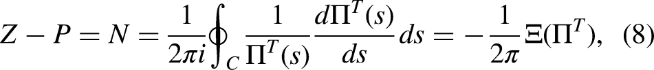
The term “direct” refers to the application of Cauchy’s argument principle directly to the common form of the dispersion relation. The term “definitive” reflects the fact that this criterion provides a sufficient and necessary condition for stability. The approach we aim to point out is in the frequency domain, so from now on we can simply assume $s=0+i\omega$ in the previous formulations. Using Cauchy’s argument principle, we can rewrite equation (8) for the given dispersion relation in equation (7) as

$${\mathcal{N}}_{{\mathrm{\Pi }}^T}={\mathcal{Z}}_{{\mathrm{\Pi }}^T}-{\mathcal{P}}_{{\mathrm{\Pi }}^T}$$

(9)

where $N_{{\mathrm{\Pi }}^T}$ , ${\mathcal{Z}}_{{\mathrm{\Pi }}^T}$ , and ${\mathcal{P}}_{{\mathrm{\Pi }}^T}$ are, respectively, the net encirclement of ${\mathrm{\Pi }}^T$ around the origin $0+0i$ when $\omega$ spans from $0$ to $\mathrm{\infty }$ , the number of RHP zeros of ${\mathrm{\Pi }}^T$ and the number of RHP poles of ${\mathrm{\Pi }}^T$ . Using Remarks 1 and 2, to ensure the thermoacoustic stability, we can rewrite equation (9) as follows:

$${\mathcal{N}}_{{\mathrm{\Pi }}^T}=0$$

(10)

It simply shows that the absence of encirclement is required to ensure stability, which can be determined by evaluation of the argument of ${\mathrm{\Pi }}^T$ ( $\mathrm{\Xi }({\mathrm{\Pi }}^T)$ ) according to equation (8).

DCS criterion based on ${\mathrm{\Pi }}^T=0$ (equation (7))

The term “conservative” reflects the fact that this criterion provides a sufficient but not necessary condition for stability. A conservative form can be introduced as well, and it may reduce the complexity of that criterion. According to equation (10), one can guarantee the absence of encirclement as follows:

$$|\mathrm{\Xi }({\mathrm{\Pi }}^T)|=\pi |\hat{\mathrm{\Xi }}({\mathrm{\Pi }}^T)|<\xi \pi ,0<\xi <1$$

(11)

where $\mathrm{\Xi }({\mathrm{\Pi }}^T)=\mathrm{\angle }{\mathrm{\Pi }}^T$ denotes the $\pi$ -wrapped argument of ${\mathrm{\Pi }}^T$ , and $\hat{\mathrm{\Xi }}({\mathrm{\Pi }}^T)=\mathrm{\Xi }({\mathrm{\Pi }}^T)/\pi$ indicates the $\pi$ -normalized form of $\mathrm{\Xi }({\mathrm{\Pi }}^T)$ . The coefficient $\xi$ can be set to any value between $0$ and $1$ . Smaller values present a higher argument margin form. For example, for $\xi =0.5$ , one can rewrite equation (11) as $\mathrm{\Re }({\mathrm{\Pi }}^T)>0$ and it stands on the fact that to make an encirclement, the value of the real part of the dispersion relation needs to become negative at a certain frequency range.

Explanation of numerical case studies

It becomes imperative to establish the primary objective of burner development as maximizing the range of stable operations for any potential (but passive) upstream and/or downstream acoustic terminations. This objective raises an important question: how can burners with their corresponding flames be compared in terms of their risk of instability?

To introduce the general idea that we are proposing to tackle this problem, the explanation will be done first on the basis of a particular example. Subsequently, its application will be used to compare two real burners in the section titled “Experimental demonstration of the application of the $\mathcal{S}$ Factor.”

For this purpose, now a set of burner TFs will be specified and the proposed analysis methodology will be applied to evaluate a ranking of the selected burners with respect to their thermoacoustic quality.

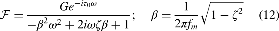
It is known that the thermoacoustic behavior of many practical flames can be described by the TF simplified to a time-delayed second-order TF with damping factor ( $\zeta$ ) as follows:

$$\mathcal{F}=\frac{G{e}^{-i{\tau }_0\omega }}{-{\beta }^2{\omega }^2+2i\omega \zeta \beta +1};\beta =\frac{1}{2\pi f_m}\sqrt{1-{\zeta }^2}$$

(12)

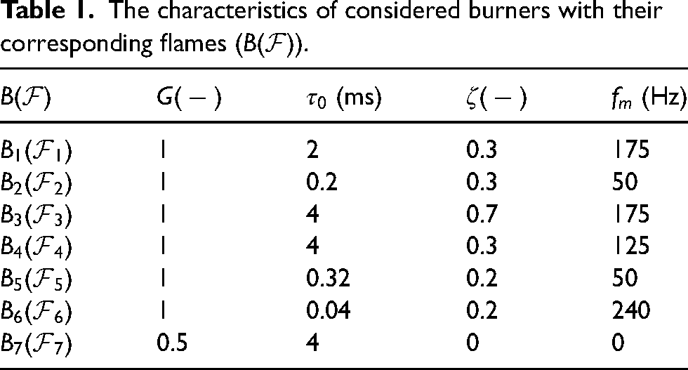
where ${\tau }_0$ and $\omega =2\pi f$ represent time delay and angular frequency, respectively. $f$ and $f_m$ indicate the frequency and corresponding overshoot frequency, which is the frequency at which the TF gain attends the maximum. To evaluate the thermoacoustic quality of the combustion system, we consider seven different acoustically transparent burners with their corresponding flames, shown in Table 1.

Table 1.

The characteristics of considered burners with their corresponding flames ( $B(\mathcal{F})$ ).

$B(\mathcal{F})$	$G(-)$	${\tau }_0$ (ms)	$\zeta (-)$	$f_m$ (Hz)
$B_1({\mathcal{F}}_1)$	1	2	0.3	175
$B_2({\mathcal{F}}_2)$	1	0.2	0.3	50
$B_3({\mathcal{F}}_3)$	1	4	0.7	175
$B_4({\mathcal{F}}_4)$	1	4	0.3	125
$B_5({\mathcal{F}}_5)$	1	0.32	0.2	50
$B_6({\mathcal{F}}_6)$	1	0.04	0.2	240
$B_7({\mathcal{F}}_7)$	0.5	4	0	0

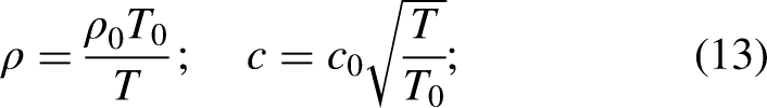
To form the transfer matrix, knowledge of upstream and downstream temperatures is required. Therefore, a fixed value of $T_1=300$  K is assumed, and a uniform temperature of $T_2=1900$  K representative of a realistic burner configuration is chosen. Density and sound velocity can be defined as a function of temperature:

$$\rho =\frac{{\rho }_0{T}_0}{T};c=c_0\sqrt{\frac{T}{T_0}}$$

(13)

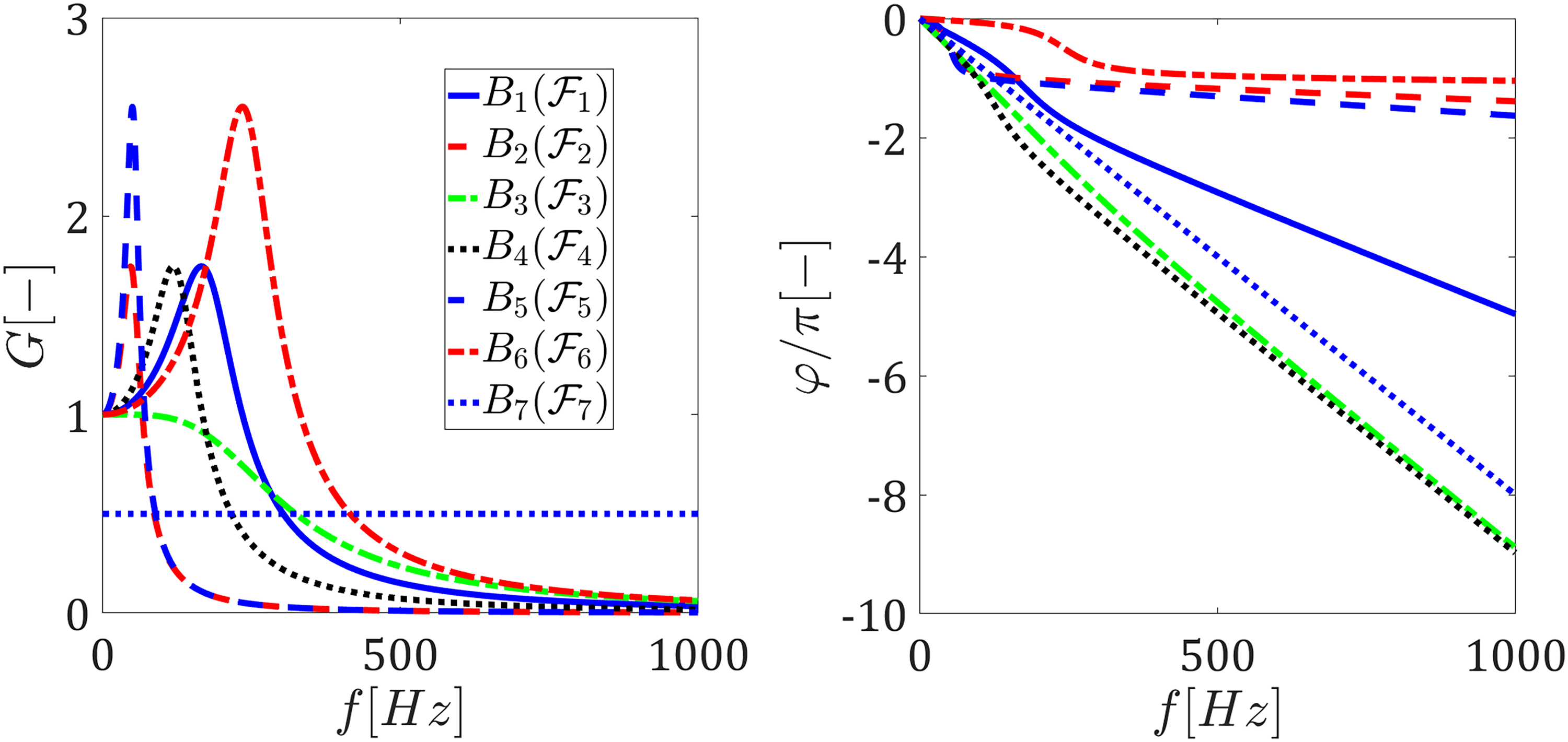
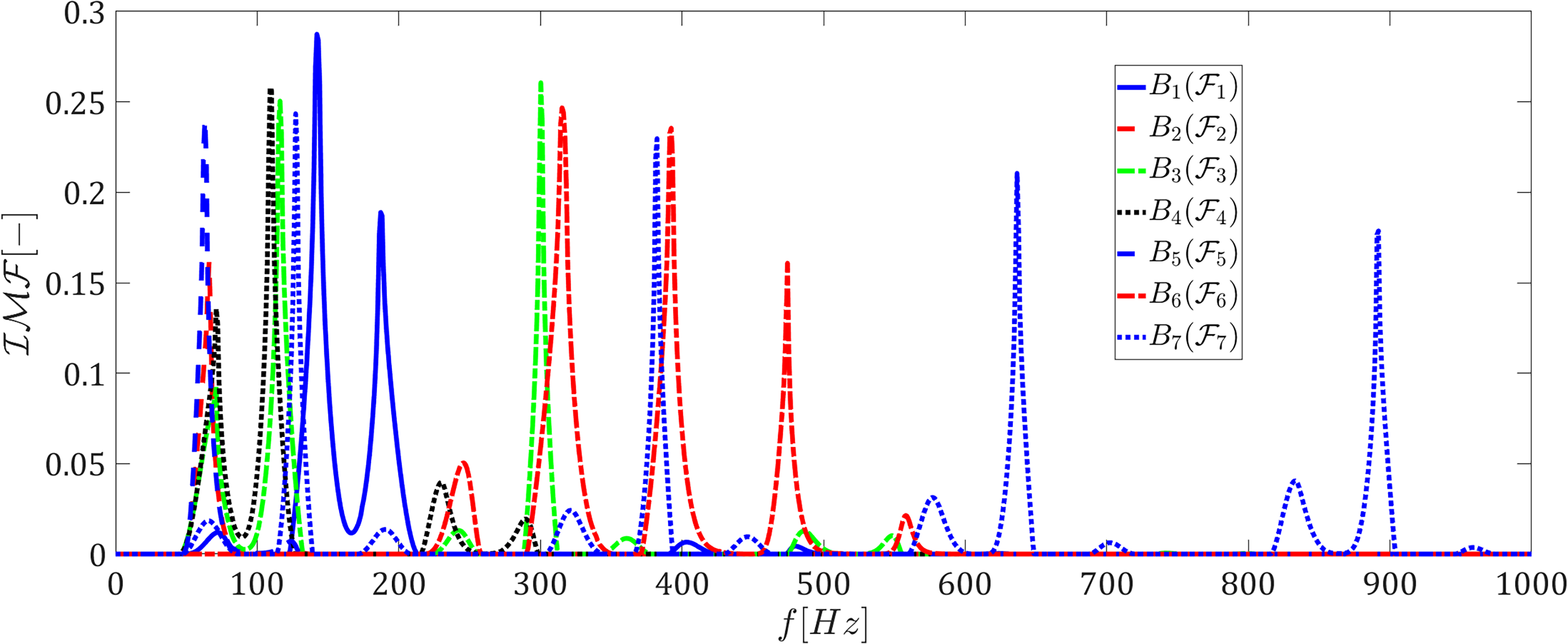
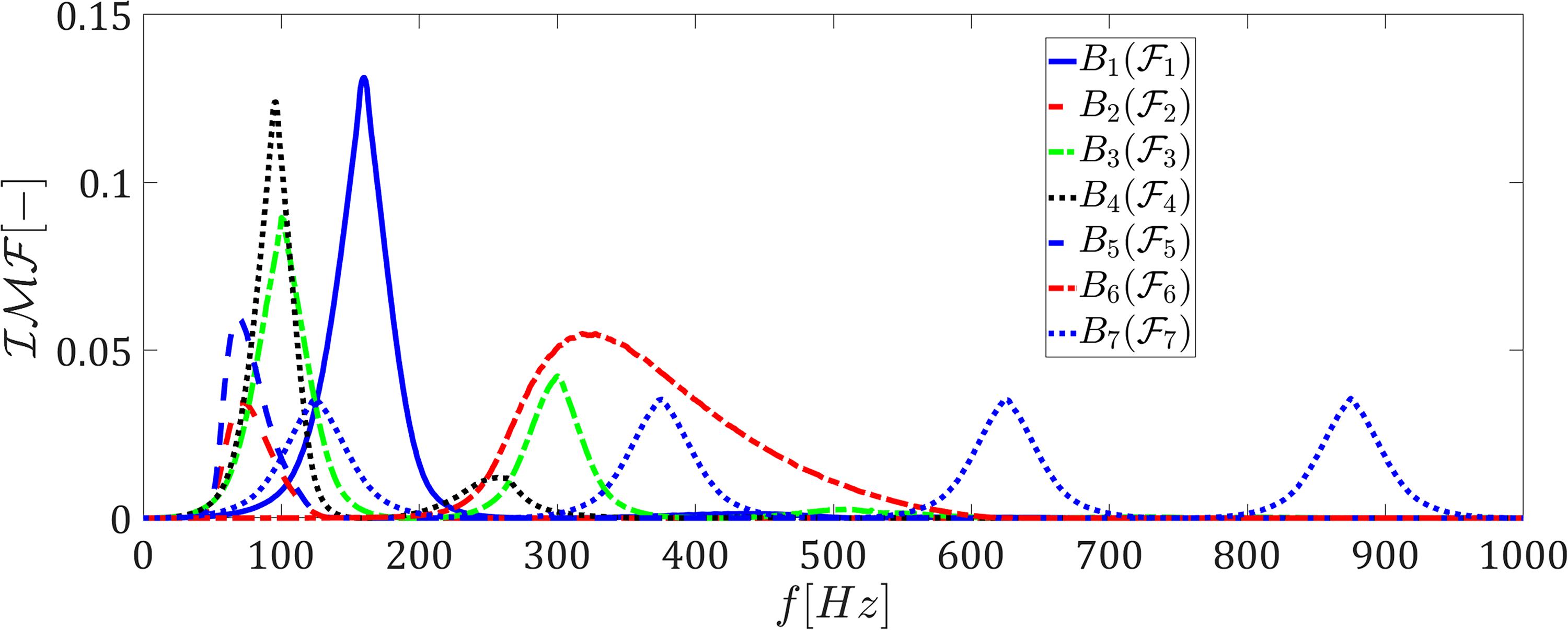
where ${\rho }_0=1.29$  kg/m³, $T_0=273$  K, and $c_0=331$  m/s. Overall, we have gathered comprehensive information about the burners and their corresponding flames (as presented in Table 1 and depicted in Figure 4).

Figure 4.

Flame transfer function of the given burners according to Table 1.

To apply the concept presented in the previous section, we consider two design scenarios that may happen in the R&D process of combustor/burner development.

First design scenario: Only half acoustic subsystem is specified

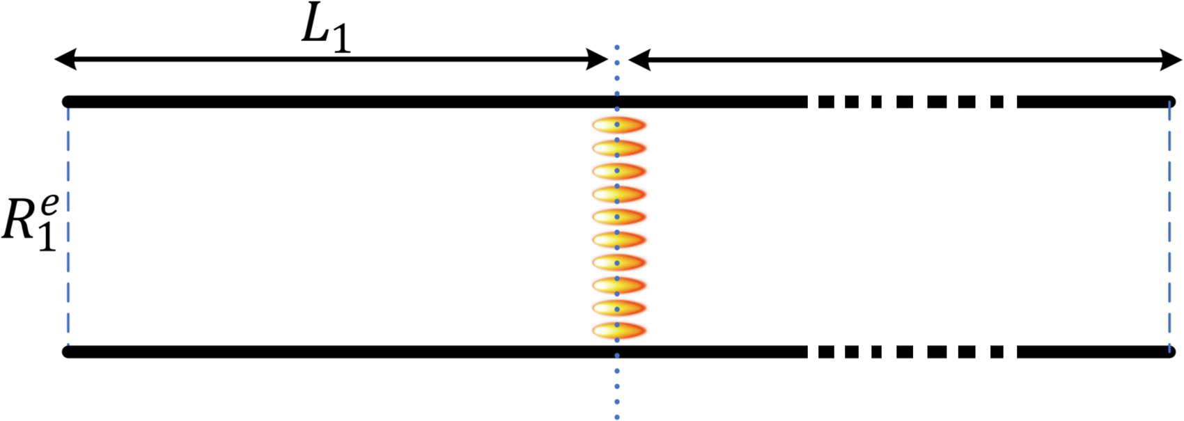
A generic thermoacoustic system can be represented by the network model depicted in Figure 1. As an illustrative benchmark case, we will examine the ducted flame test configuration depicted in Figure 5, which represents a duct-flame-duct with an upstream length of $L_1=2$  m. The end terminations upstream are assumed to be frequency-independent and have purely real end reflections $R_1^e=0.7$ . The total acoustic reflection upstream of the flame can be treated as a lumped parameter:

$$R_{\mathrm{up}}=R_1^e{e}^{-2i\omega L_1/c_1}$$

(14)

The practical difficulties in assessing the downstream (hot side) reflection coefficient often lead to a burner development without prior knowledge of the downstream acoustics within the intended industrial system. Therefore, suppose there is a shortage of available data regarding downstream acoustics. Consequently, our primary objective is to assess the thermoacoustic quality of various burners along with their corresponding flames when the upstream acoustics is known/specified, but the downstream acoustics is not. For the sake of simplicity, yet without loss of generality, we here assume that these burners are acoustically transparent. This assumption implies that the transfer matrix of the burners is a unity matrix. Consequently, we can conveniently posit the absence of any additional acoustic elements between the upstream termination and the flame. The aim is to categorize the burners based on their susceptibility to thermoacoustic instability when integrated with the provided upstream termination.

Figure 5.

Sketch of a uniform duct-flame-duct geometry with unspecified downstream acoustic.

Second design scenario: None of the upstream and downstream acoustic subsystems are specified

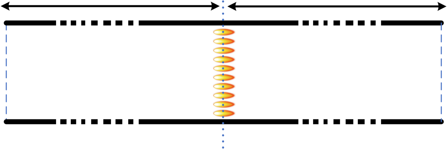
In this scenario, as shown in Figure 6, we assume a lack of information regarding the location where the burners/combustors will be positioned, leading to unknown acoustic properties of both upstream and downstream terminations. Consequently, our primary objective is to evaluate the thermoacoustic quality of various acoustically transparent burners and their corresponding flames, irrespective of any specified terminations.

Figure 6.

Sketch of a generic thermoacoustic system with unspecified upstream and downstream acoustic subsystems.

Results and discussion on the numerical case studies

In this study, we utilize the key aspects of the DCS stability criteria to establish a quality factor (figure-of-merit) for thermoacoustics. As shown in equation (11), the DCS criterion incorporates an overall argument margin parameter ( $\xi$ ), which can be set as a threshold. This parameter offers flexibility in adjusting the level of conservatism of the criterion, allowing for the investigation of a system’s robustness. However, the analysis of system robustness is beyond the scope of this article.

First design scenario: Only half acoustic subsystem is specified

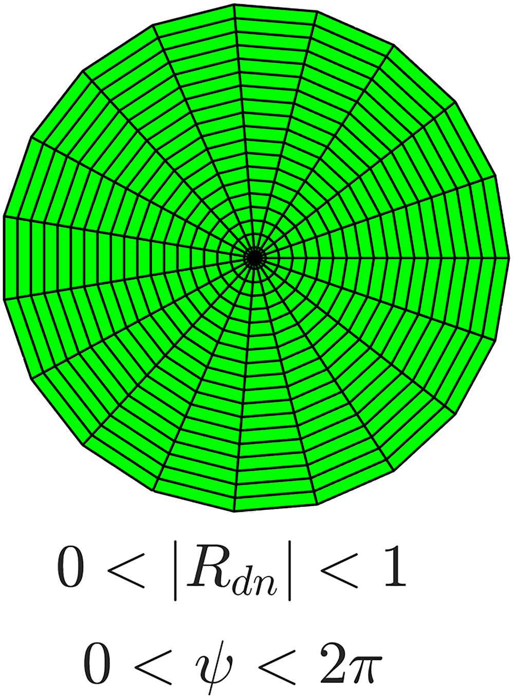
To apply this methodology, we introduce the concept of a stability map. By utilizing the known reflection coefficients of the upstream termination and the burners, along with their associated flame TFs, for each fixed frequency from the range of interest, we scan all possible values of $R_{\mathrm{dn}}$ within the unit circle in the complex domain (see Figure 7).

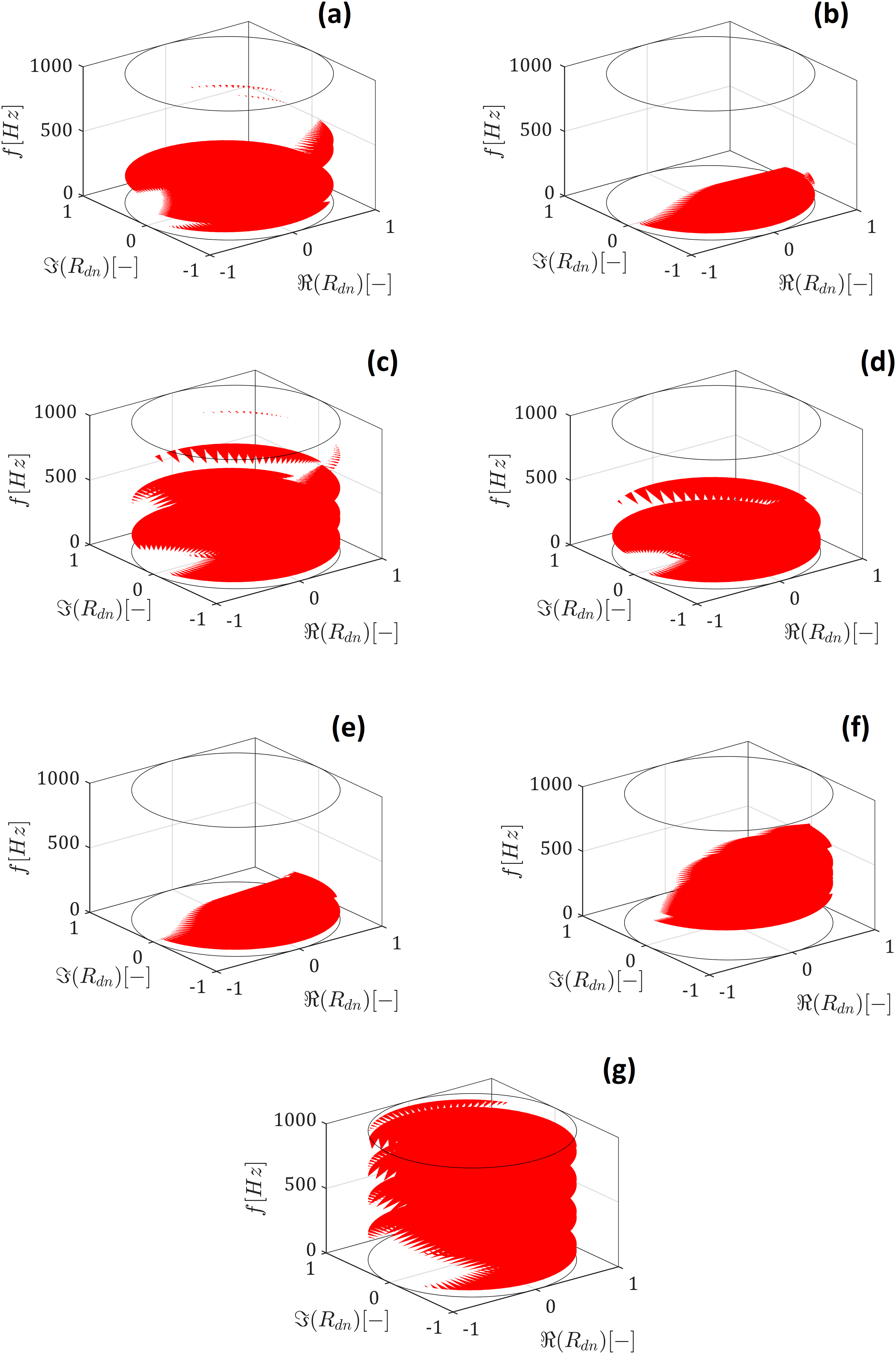
We then identify the region where the condition stated in equation (11) is violated and mark it in red. This region is referred to as the “unsafe” zone, indicating that if a downstream termination exists with a reflection coefficient falling within this red region at a specific frequency, thermoacoustic instability may occur according to the DCS criterion. Through that, we generate a comprehensive stability map for each frequency. Figure 8 presents a three-dimensional (3D) representation of this stability map for different burners in combination with the known upstream termination. The $x$ -axis and $y$ -axis correspond to the real and imaginary values, respectively, of all possible downstream reflection coefficient values within the unit circle, while the $z$ -axis represents the frequency range of interest. Thus, each constant $z$ -slice of this 3D stability map represents a stability map associated with a specific frequency. To generate these graphs, we chose a threshold value of $\xi =0.95$ and applied the DCS criterion (equation (11)) to identify values of $R_{\mathrm{dn}}$ within the unit circle that violate this condition. These violating values were marked in red, representing the region in which the downstream reflection coefficient, among all possibilities within the unit circle, could potentially lead to system instability based on this conservative stability criterion. The stability map varies along the frequency axis, highlighting the importance of analyzing the stability map at different frequencies. This provides valuable insights into the system behavior and paves the way for a new approach to introduce a figure-of-merit. To enable a more comprehensive visualization, the 3D stability charts have been saved as individual video files, with each frame representing a frequency slice. For a detailed examination and access to these videos, please refer to the supplemental material accompanying this article.

Figure 7.

Schematic of a grid/mesh showing all possible values for downstream reflection coefficients.

Figure 8.

The three-dimensional (3D) stability maps of the given subsystem are equipped with different burners with their corresponding flames: (a) $B_1({\mathcal{F}}_1)$ , (a) $B_2({\mathcal{F}}_2)$ . (c) $B_3({\mathcal{F}}_3)$ . (d) $B_4({\mathcal{F}}_4)$ . (e) $B_5({\mathcal{F}}_5)$ , (f) $B_6({\mathcal{F}}_6)$ , and (g) $B_7({\mathcal{F}}_7)$ .

The instability manifestation fraction ( $\mathcal{I}\mathcal{M}\mathcal{F}$ )

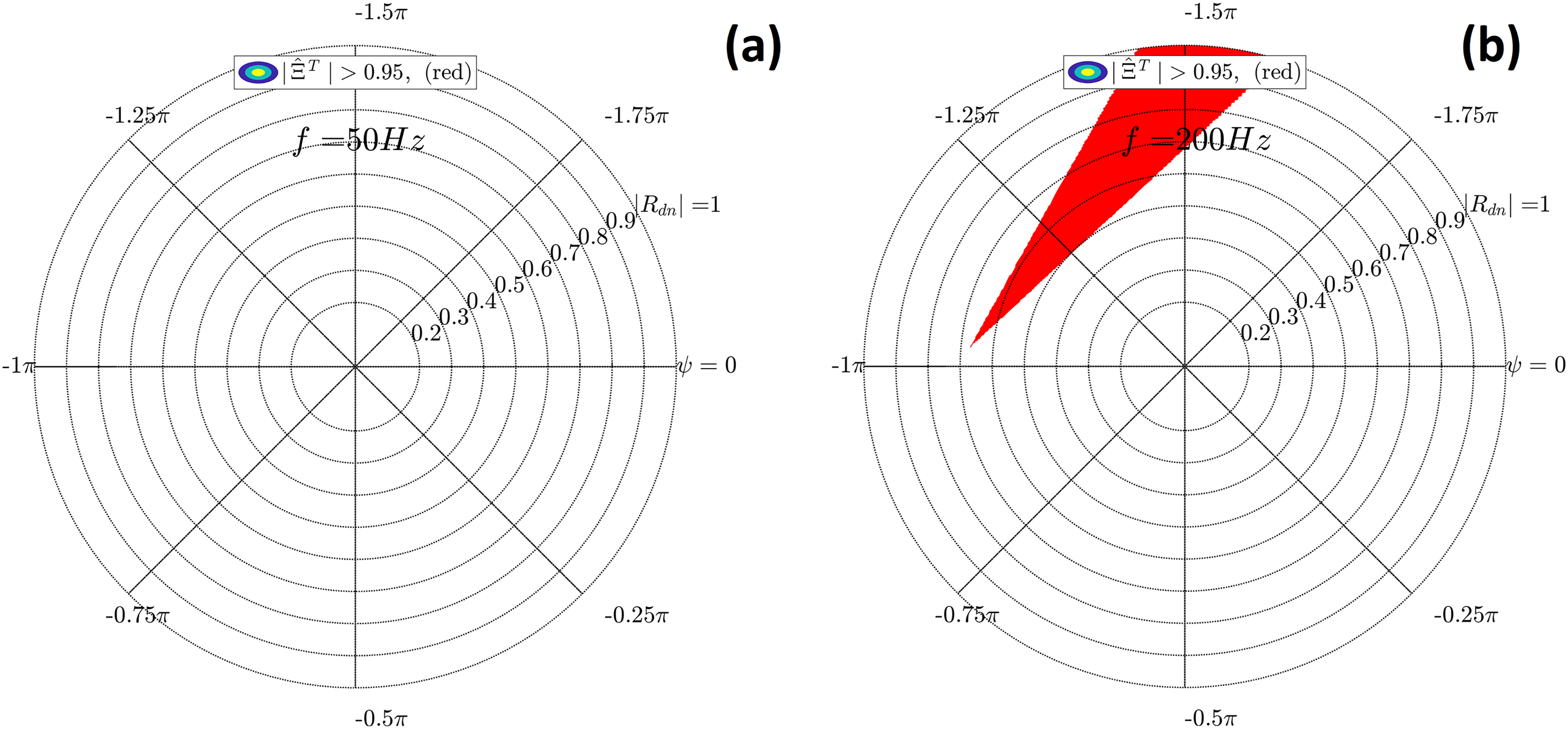
Figure 9 presents two frames extracted from “video-DCS-Burner1,” showcasing the stability maps of the subsystem equipped with burner 1 and its corresponding flame TF at frequencies of 50 and 200 Hz. In these charts, the dotted circles and straight dotted lines inside the unit circle represent the iso-modulus and iso-phase downstream reflection coefficients, respectively. Figure 9(a) shows that the entire unit circle represents safe values that do not lead to system instability. Consequently, if we define a function called the $\mathcal{I}\mathcal{M}\mathcal{F}$ as the ratio of the number of red mesh cells to the total number of cells inside the unit circle, at the considered frequency of 50 Hz, we can say $\mathcal{I}\mathcal{M}\mathcal{F}$ is equal to $0$ . On the other hand, according to Figure 9(b), an unsafe zone in red is observed, representing the values of downstream reflection coefficient at the frequency 200 Hz that should be avoided due to the risk of thermoacoustic instability, resulting in a nonzero risk of instability manifestation.

Figure 9.

The stability map of the subsystem equipped with $B_1({\mathcal{F}}_1)$ at the frequencies (a) $f=50$  Hz and (b) $f=200$  Hz.

Now, with the availability of stability maps across the entire frequency range, it becomes possible to calculate the $\mathcal{I}\mathcal{M}\mathcal{F}$ throughout the frequency range. Figure 10 presents a comparison of the $\mathcal{I}\mathcal{M}\mathcal{F}$ for different burners with flames when embedded in a combustion system with a given upstream termination ( $R_{\mathrm{up}}$ ). This graph offers valuable insights into the flames’ stabilization. In scenarios where a combustion system experiences thermoacoustic instability, and the frequencies of instabilities are known and measurable, this graph can assist in selecting a replacement burner with a lower risk of instability within that frequency range, even without information on the downstream acoustics. For example, if thermoacoustic instability occurs at the frequency of 100 Hz, choosing burner 6 with the corresponding flame TF ${\mathcal{F}}_6$ would be a more prudent decision compared to the other burners, as burner 6 exhibits a significantly lower risk of instability around this frequency. It is important to note that we used the phrase around with emphasis (not at), as the $\mathcal{I}\mathcal{M}\mathcal{F}$ has been computed in the imaginary frequency domain (i.e. zero growth rate $\sigma =0$ ). Therefore, one should keep in mind the difference between analysis in the imaginary frequency domain and the complete complex domain.

Figure 10.

The instability manifestation fraction versus frequency for the given subsystems.

The thermoacoustic quality factor $\mathcal{S}$ for figure-of-merit

The $\mathcal{I}\mathcal{M}\mathcal{F}$ versus frequency alone is insufficient to serve as a single performance metric for globally comparing and ranking different burners based on their risk of instability, which constitutes the primary objective of this article. In this subsection, we endeavor to address this limitation by introducing a stability quality factor $\mathcal{S}$ as a figure-of-merit.

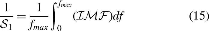
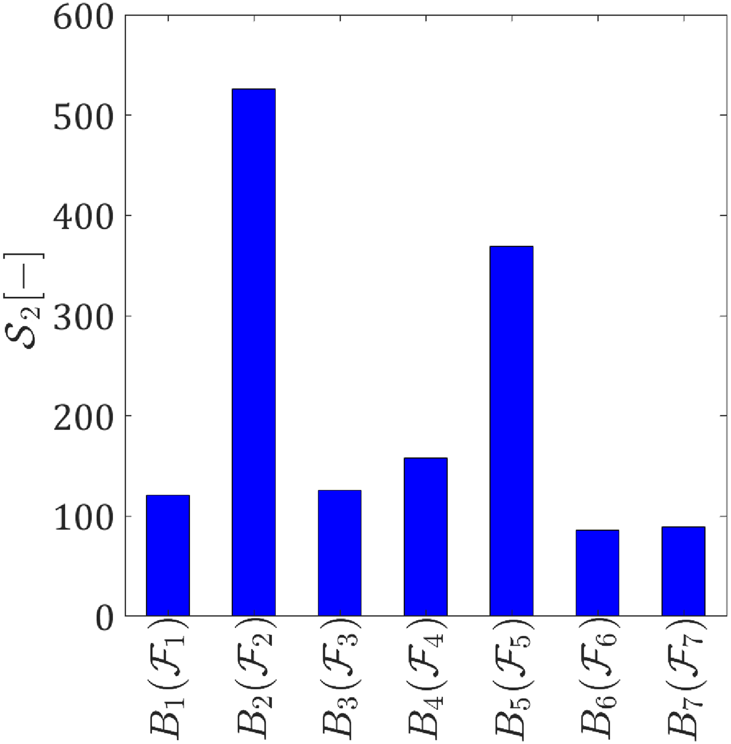
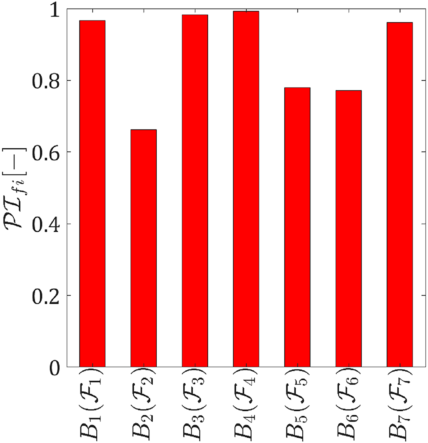
In Figure 10, we obtained the $\mathcal{I}\mathcal{M}\mathcal{F}$ distribution over the frequency range for different subsystems. To derive a quality factor for comparison, one possible approach is to calculate the relative area fraction under the $\mathcal{I}\mathcal{M}\mathcal{F}$ curves. This can be represented as,

$$\frac{1}{{\mathcal{S}}_1}=\frac{1}{f_{max}}{\int }_0^{f_{max}}(\mathcal{I}\mathcal{M}\mathcal{F})df$$

(15)

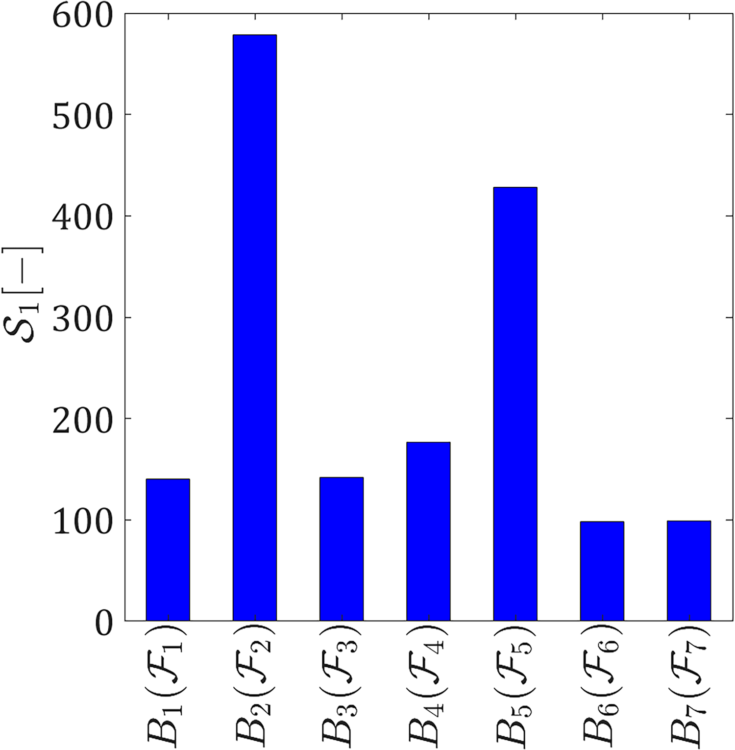
where $f_{max}$ is the maximum frequency of interest. The resulting ${\mathcal{S}}_1$ represents the geometric mean of the $\mathcal{I}\mathcal{M}\mathcal{F}$ values and reflects the overall change in stability. However, it is important to note that the numerical value of the stability quality factor for a single burner does not have a direct linear correlation with other burners. For example, in Figure 11, we can observe that the stability quality factor for burner 1 is more than three times smaller than that for burner 2. However, it would be incorrect to interpret this as burner 1 being three times worse than burner 2. This quality factor is a relative measure that allows for the comparison of different burners based on their likelihood of stability. Additionally, as expected, burner 5 demonstrates better stability than burner 6. In general, the ranking of different burners based on their stability probability, from highest to lowest, would be: burner 2, burner 5, burner 4, burners 1 and 3 (similar), followed by burners 6 and 7 (similar and close to each other).

Figure 11.

The normalized stability quality factor obtained from the direct conservative stability criterion using integrating the instability manifestation fraction ( $\mathcal{I}\mathcal{M}\mathcal{F}$ ) over the entire frequency range of interest in the first design scenario.

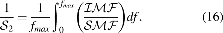
In some rare cases, when the value of $\mathcal{I}\mathcal{M}\mathcal{F}$ approaches unity within a small frequency range, the integration method used to calculate ${\mathcal{S}}_1$ can potentially lead to misleading results. This is because if there exists even a narrow frequency range where $\mathcal{I}\mathcal{M}\mathcal{F}$ is unity, it indicates system instability regardless of the behavior in other frequency ranges. To address this concern, an alternative stability factor can be considered as,

$$\frac{1}{{\mathcal{S}}_2}=\frac{1}{f_{max}}{\int }_0^{f_{max}}\left(\frac{\mathcal{I}\mathcal{M}\mathcal{F}}{\mathcal{S}\mathcal{M}\mathcal{F}}\right)df$$

(16)

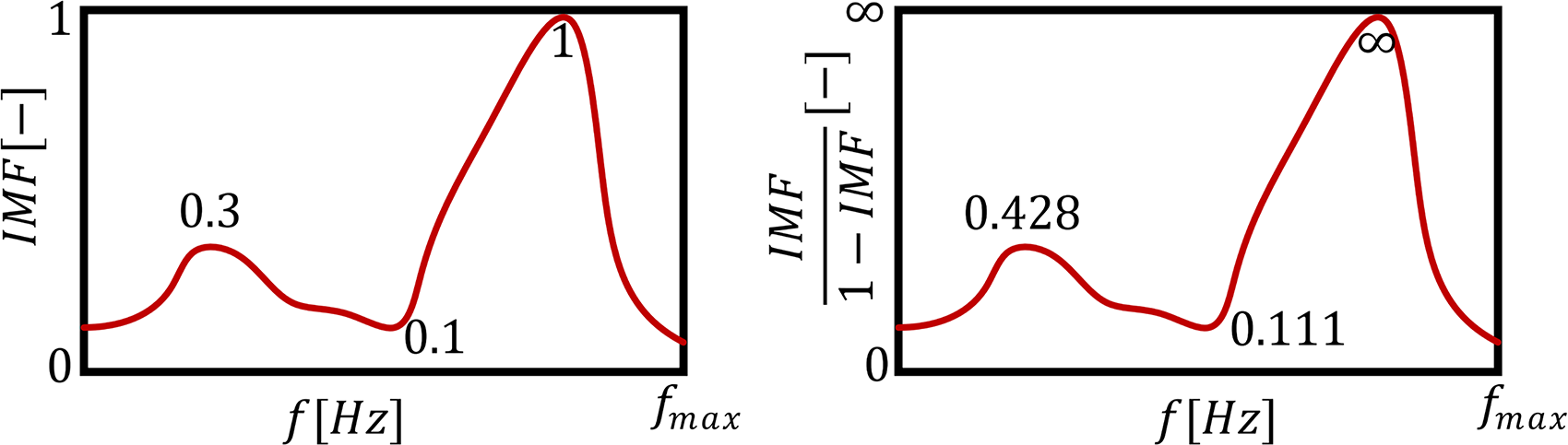
In the equation $\mathcal{S}\mathcal{M}\mathcal{F}=1-\mathcal{I}\mathcal{M}\mathcal{F}$ , $\mathcal{S}\mathcal{M}\mathcal{F}$ denotes the stability manifestation fraction. Figure 12 illustrates a critical scenario, emphasizing how mapping from $\mathcal{I}\mathcal{M}\mathcal{F}$ to $\mathcal{I}\mathcal{M}\mathcal{F}/\mathcal{S}\mathcal{M}\mathcal{F}$ can resolve the issue of ${\mathcal{S}}_1$ . When $\mathcal{I}\mathcal{M}\mathcal{F}$ is small, $\mathcal{I}\mathcal{M}\mathcal{F}\approx \mathcal{I}\mathcal{M}\mathcal{F}/\mathcal{S}\mathcal{M}\mathcal{F}$ ; whereas in the frequency band where $\mathcal{I}\mathcal{M}\mathcal{F}$ is around unity, $\mathcal{I}\mathcal{M}\mathcal{F}/\mathcal{S}\mathcal{M}\mathcal{F}\approx \mathrm{\infty }$ . Consequently, ${\mathcal{S}}_2$ is calculated as zero, meeting the objective.

Figure 12.

A clarification example on mapping from $\mathcal{I}\mathcal{M}\mathcal{F}$ to $\mathcal{I}\mathcal{M}\mathcal{F}/\mathcal{S}\mathcal{M}\mathcal{F}$ . $\mathcal{I}\mathcal{M}\mathcal{F}$ : instability manifestation fraction; $\mathcal{S}\mathcal{M}\mathcal{F}$ : stability manifestation fraction.

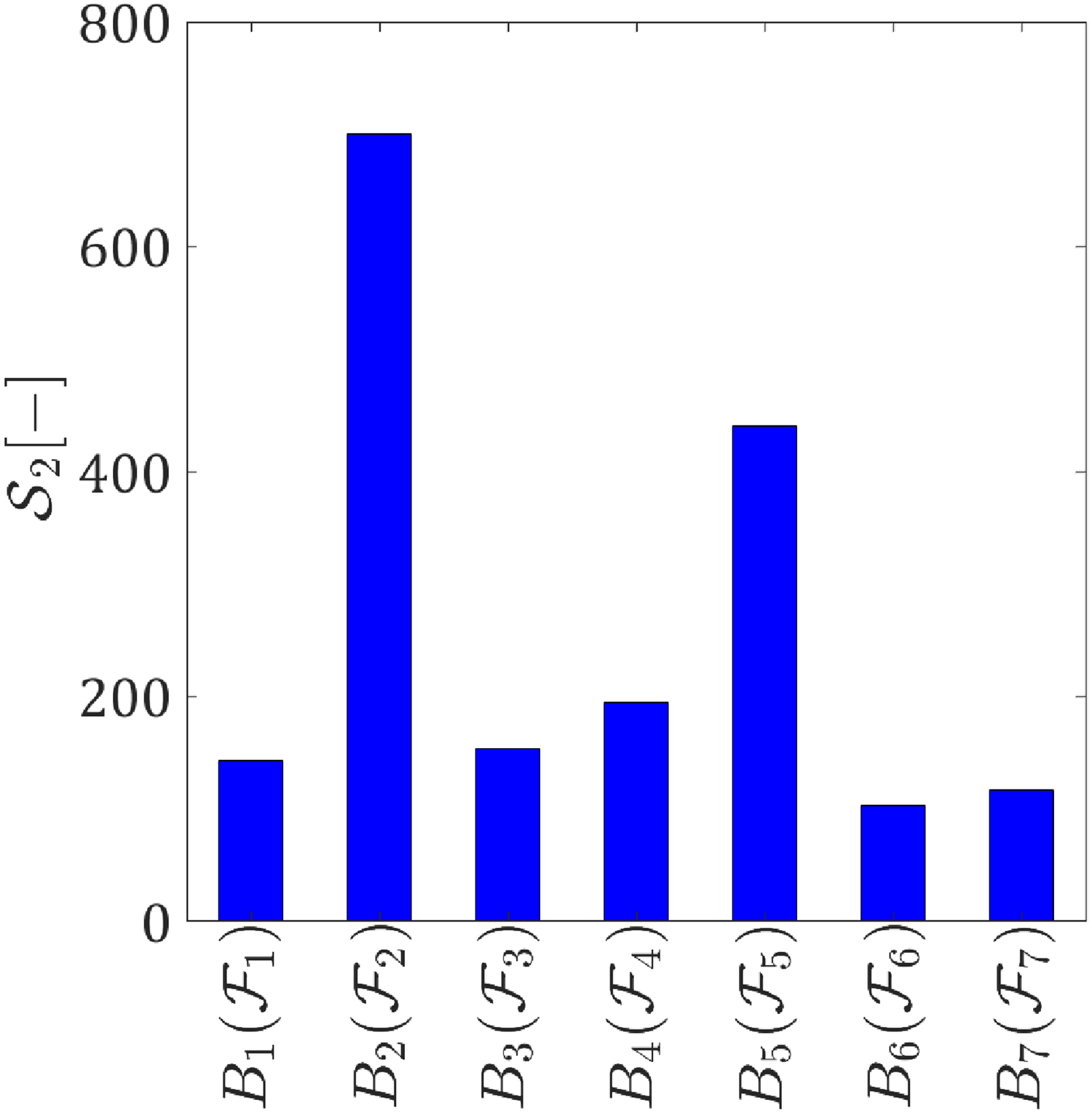
Figure 13 offers a comparison of subsystems equipped with different burners using ${\mathcal{S}}_2$ . Interestingly, the values of this stability quality factor closely align with the values of ${\mathcal{S}}_1$ , maintaining the same burner ranking. This suggests that ${\mathcal{S}}_2$ effectively resolves the issue of misleading results arising from narrow frequency ranges with unity $\mathcal{I}\mathcal{M}\mathcal{F}$ values. Therefore, ${\mathcal{S}}_2$ can be recommended as a robust stability factor, providing reliable insights for comparing and ranking the thermoacoustic quality of different burners in the system.

Figure 13.

The normalized stability quality factor obtained from the direct conservative stability criterion using integrating the instability manifestation fraction ( $\mathcal{I}\mathcal{M}\mathcal{F}$ ) functions by considering the weighted function over the entire frequency range of interest in the first design scenario.

Second design scenario: None of the upstream and downstream acoustic subsystems are specified

In the first design scenario, we assumed the upstream reflection coefficient of a generic combustion system is given, while no knowledge of the downstream reflection coefficient is available. We introduced the concept of the $\mathcal{I}\mathcal{M}\mathcal{F}$ and formulated the stability quality factor to serve as a figure-of-merit in thermoacoustic instability.

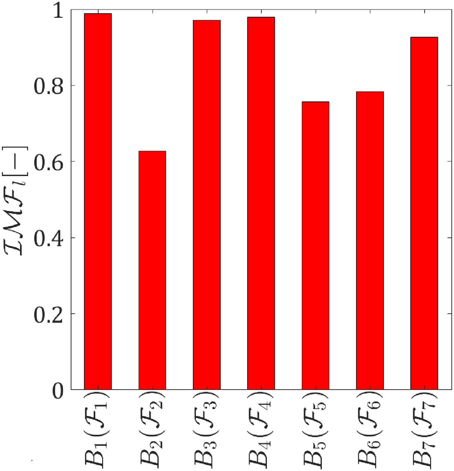
Now, we briefly address the second design scenario, where none of the upstream or downstream acoustic subsystems are specified. In this case, we need to generate a four-dimensional (4D) mesh to consider all possible combinations between $R_{\text{up}}$ and $R_{\text{dn}}$ at each frequency. Generally, a 4D computational domain can be generated using a standard function in Matlab called ndgrid. Despite the conceptual similarity of the work flows associated with these two design scenarios, the difficulties in visualizing geometrical features in 4D space limit the possibilities for intuitive interpretations and graphical representation of the obtained data. Accordingly, only cumulative indicators and/or projections on low-dimensional subspaces can be analyzed. Figure 14 illustrates the $\mathcal{I}\mathcal{M}\mathcal{F}$ for different burners with their corresponding flames. One can then calculate the stability quality factor, as shown in Figure 15. Interestingly, the values are slightly different from the values obtained in the first design scenario where the upstream reflection coefficient $R_{\text{up}}$ was specified. However, the comparison reveals that the order of burners based on their thermoacoustic quality is quite similar to the previous design scenario. It is worth pointing out that an exact match is not necessary and generalization of this observation should be avoided.

Figure 14.

The instability manifestation fraction versus frequency for various burners with their corresponding flames.

Figure 15.

The normalized stability quality factor obtained using integrating the $\mathcal{I}\mathcal{M}\mathcal{F}$ functions over the entire frequency range of interest in the second design scenario.

Extension of the analysis for the case of semi-specified upstream and downstream acoustic subsystems

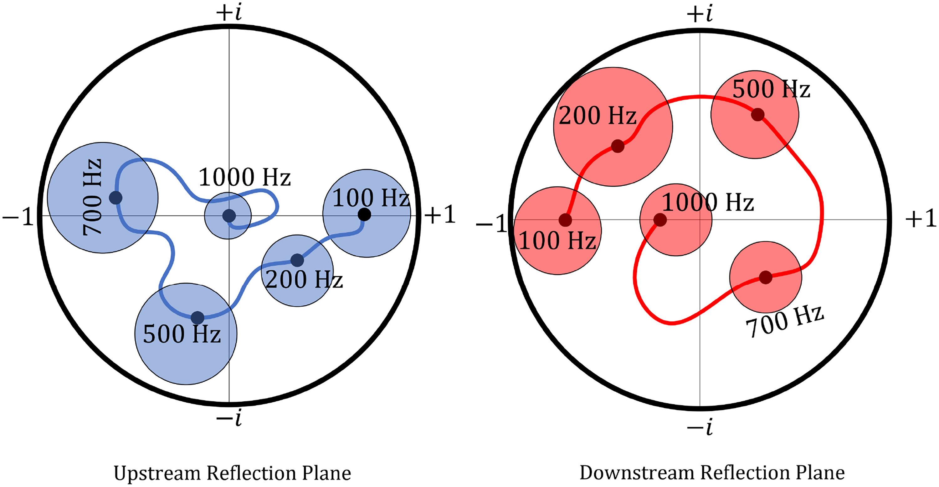
In practical situations, partial knowledge can be available of where the burners will be installed, for instance, in a domestic central boiler of a certain type. Therefore, we can approximately determine the upstream and downstream acoustic reflection coefficient. However, due to uncertainties in the characterization of the termination, potentially un-modeled physics in numerical evaluations, and variations in the values of upstream and downstream acoustic reflections caused by, for example, changing thermal power, and so on, it becomes crucial to find a figure-of-merit taking into the consideration bounds imposed by the partial knowledge which are reflected by the semi-specified regions inside the upstream and downstream reflection coefficient complex unit circles. This scenario is illustrated in Figure 16, where the blue and red lines indicate the approximate reflection coefficient in the upstream and downstream complex unit circle plane over the entire frequency of interest, respectively. The analysis methodology introduced above can be readily extended to include the consideration of prior knowledge about the localization of allowable reflection coefficients. In this situation, to evaluate the thermoacoustic quality of different burners (with their flame), we can define regions of interest at different frequencies, as depicted with the colored circles in Figure 16. Next the calculation of $\mathcal{I}\mathcal{M}\mathcal{F}$ should be performed only inside the specified region of interest for all frequencies. Accordingly, the stability quality factor will indicate the burner property filtered by the specific class of its acoustic embedding. This approach allows for a narrow focus and study of the specific application under consideration.

Figure 16.

Schematics of situation with semi-specified upstream and downstream acoustic subsystems.

Discussion on the limitation and potential misinterpretations of MC simulations against DCS criterion in the context of figure-of-merit

The methodology of the system analysis and the developed approach to evaluate the burner with flame figure-of-merit can be compared with the other approaches proposed before, particularly, with the MC-based evaluations of probability of (in-)stability. This comparative study allows getting deeper insight into the essence of both approaches and elucidates some shortcomings of them. In this subsection, we seek to address the potential issues that may arise when utilizing MC simulations as an alternative approach for establishing a figure-of-merit in the context of thermoacoustic stability. We will illustrate these challenges using a similar example discussed in the first design scenario.

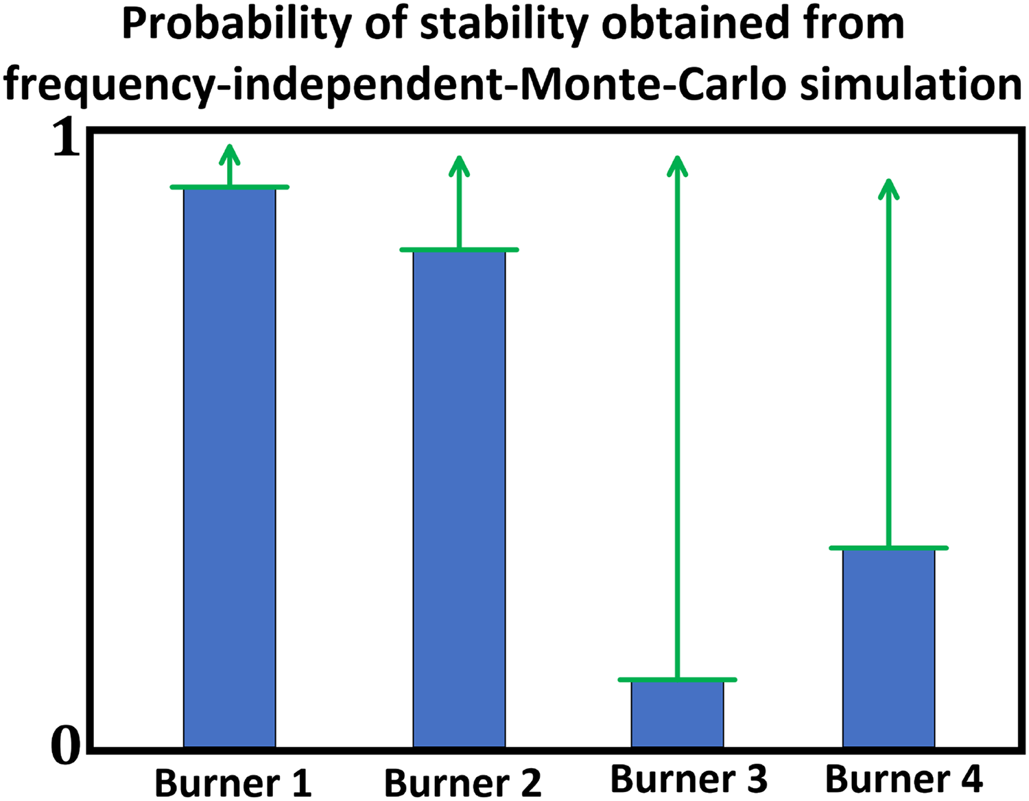
In a previous study by Kornilov et al., ¹³ the possibility of utilizing an MC simulation approach called frequency-independent reflection coefficients based MC (FIRC-MC) simulation was investigated. This approach involves randomly selecting a large set of FIRC and subsequently solving the dispersion relation each time to assess the system’s stability. The aim is to obtain a single value for the $\mathcal{P}\mathcal{I}$ , which serves as a quality factor. The $\mathcal{P}\mathcal{I}$ is calculated as the ratio of the number of unstable cases to the total number of examined cases. For more comprehensive details, please refer to Kornilov and De Goey. ¹³ To make a general comparison of the burners, we conducted MC simulations and acquired the corresponding $\mathcal{P}\mathcal{I}$ values, as shown in Figure 17.

Figure 17.

The probability of instability obtained from frequency-independent reflection coefficients based Monte Carlo simulations based on randomly chosen frequency-independent downstream reflection coefficients.

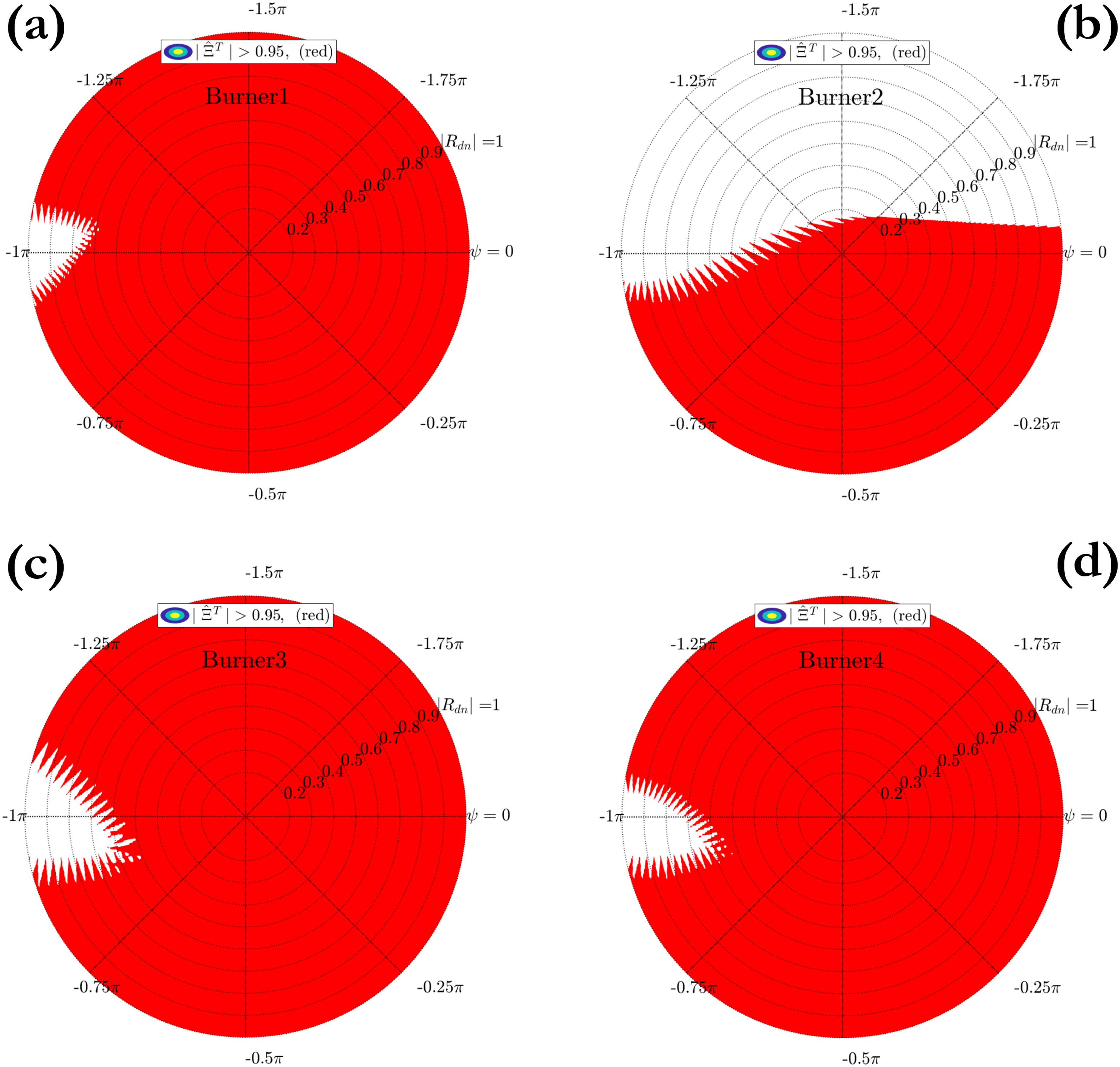
Upon initial consideration, FIRC-MC simulations may appear as a viable option for obtaining reference data for comparison. However, through our analysis, we demonstrate that FIRC-MC simulations yield an excessively conservative evaluation, which raises the question of whether this approach is appropriate for reliable comparisons. To illustrate the limitations of FIRC-MC, we aggregate the 3D stability maps obtained from the DCS criterion, as depicted in Figure 8, into a top-down view. The resulting lumped stability map is presented in Figures 18 and 19. By defining the global $\mathcal{I}\mathcal{M}\mathcal{F}$ based on the aggregated stability map as the ratio of the red meshes to the total mesh number inside the unit circle, we obtain a global $\mathcal{I}\mathcal{M}\mathcal{F}$ value for comparison with the $\mathcal{P}\mathcal{I}$ obtained from the FIRC-MC simulations. A comparative analysis of Figures 17 and 20 when performed burner by burner reveals a close alignment between the obtained $\mathcal{P}\mathcal{I}$ values. While this does not directly address the main problem, it leads to two significant conclusions. Firstly, the $\mathcal{P}\mathcal{I}$ values obtained from the DCS criterion exhibit good agreement with those obtained from the FIRC-MC simulations. This suggests that the DCS approach is not overly conservative and indicates that when the argument of the dispersion relation approaches the vicinity of $-\pi$ , the occurrence of encirclement in subsequent frequencies becomes highly likely. Secondly, upon examining the 3D stability maps of different burners in Figure 8, it is evident that the unsafe region moves extensively along the frequency axis within the unit circle. This results in a relatively small safe region in the aggregated stability map, as shown in Figures 18 and 19. From this observation, it is clear that FIRC-MC simulations, in general, have many similarities with the result obtained from the aggregated stability map of the DCS method and therefore, for many cases may lead to wrong conclusions regarding the thermoacoustic quality of the given burner with flame.

Figure 18.

The lumped stability map from top view in three-dimensional (3D) stability maps along the frequency axis for all burners 1–4.

Figure 19.

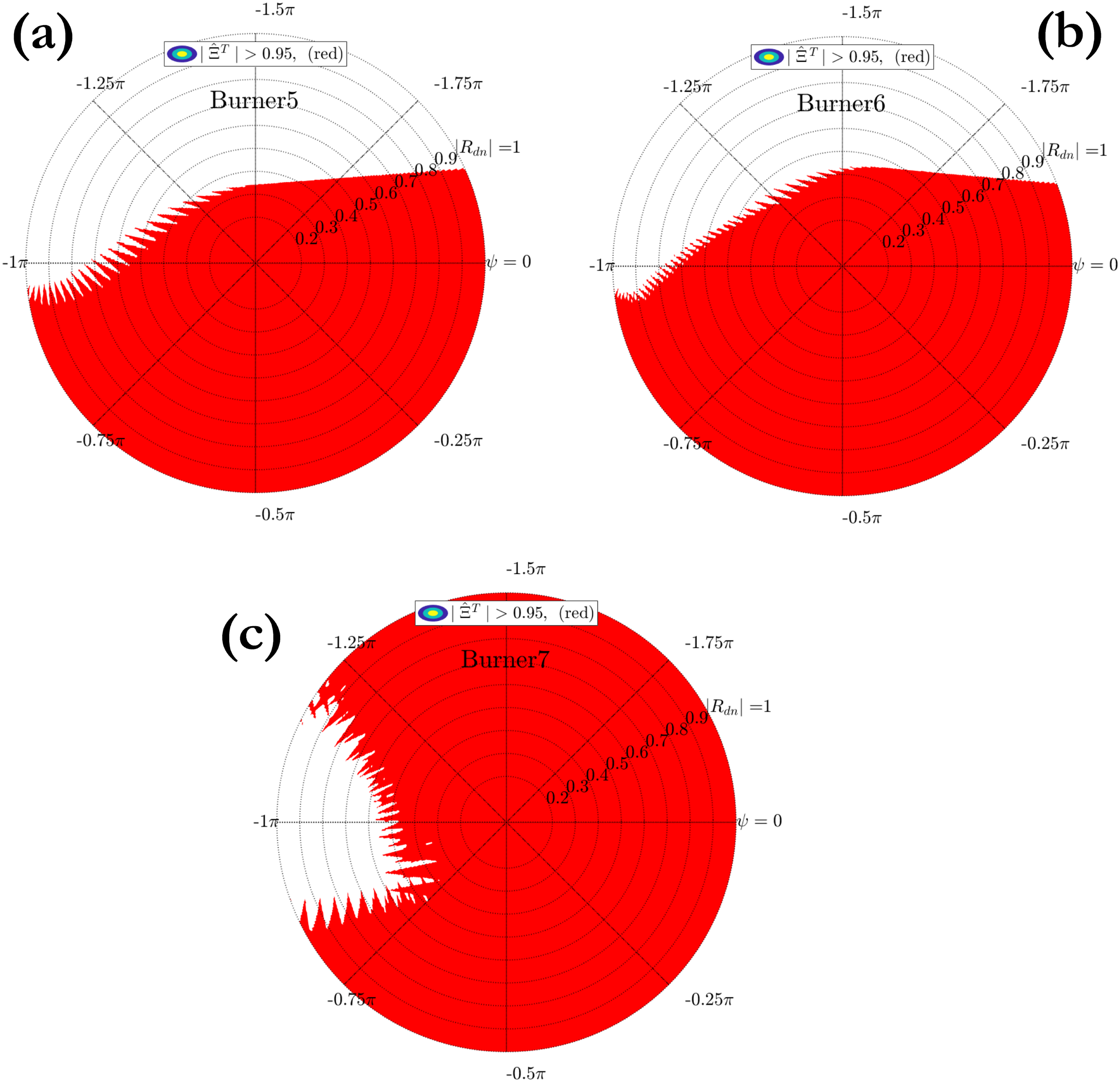
The lumped stability map from top view in three-dimensional (3D) stability maps along the frequency axis for all burners 5–7.

Figure 20.

The overall instability manifestation fraction obtained from lumped stability map in the direct conservative stability criterion.

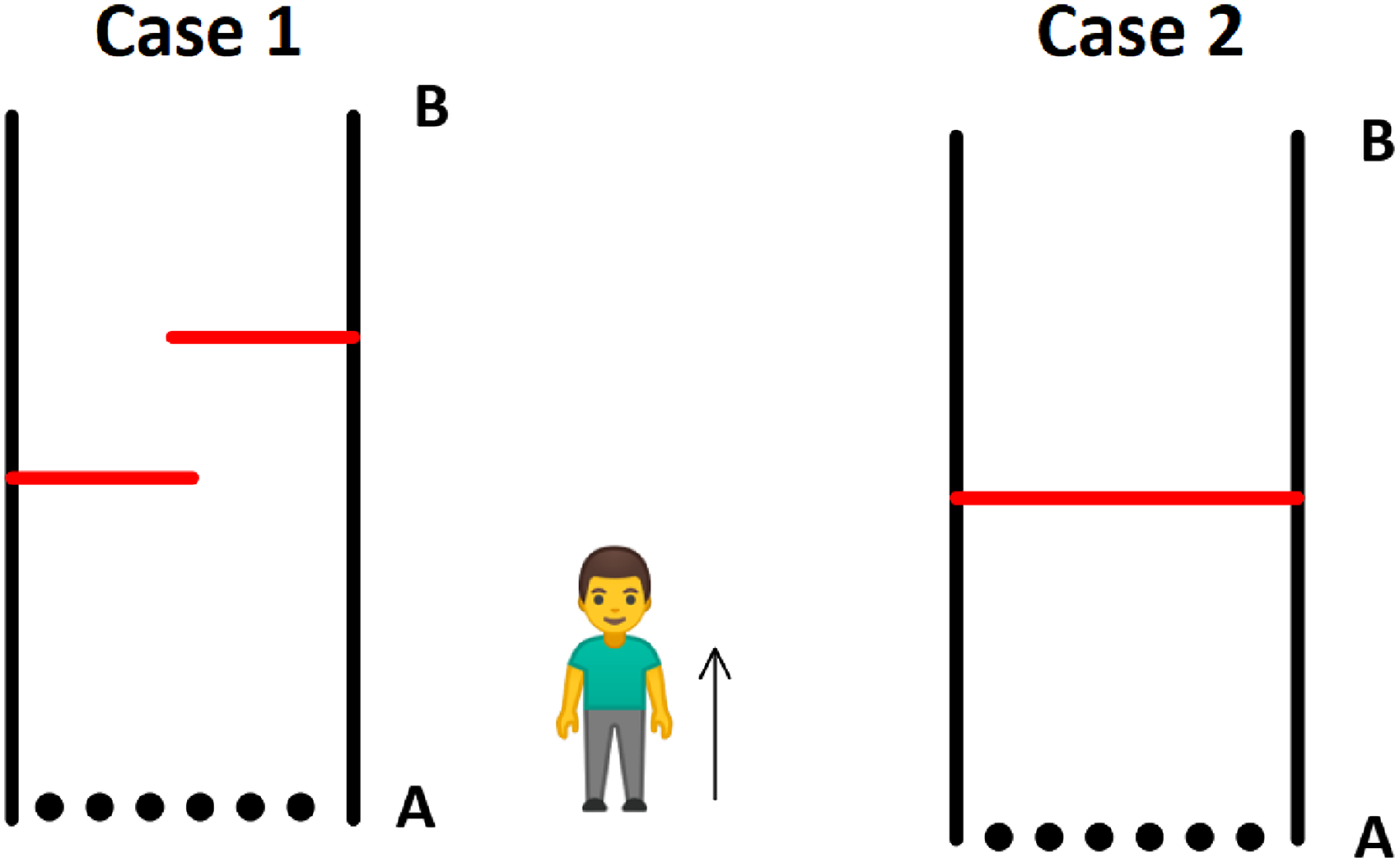
To develop an intuition regarding the issue with FIRC-MC simulations, an analogy as one represented by the scenario illustrated in Figure 21 is presented. Here, two identical canals with different wall geometries are considered. If a person is forced to start from different black points on side A to reach side B, restricted to moving straight forward without turning or going back, it is apparent that the probability of reaching point B from A, ${\mathcal{P}}_{A\to B}$ , is zero. The probability is calculated as zero for both cases, but if the motion is not limited to straight lines then there are many choices to navigate around the walls in the first case, while the side wall entirely blocks the canal in the second case, resulting in ${\mathcal{P}}_{A\to B}$ being zero regardless of the defined motion condition. This analogy illustrates that imposing constraints on movement leads to an overly conservative perspective and may result in an incorrect evaluation. This mirrors the situation in FIRC-MC simulations, where the length of the canal represents the frequency axis and the walls resemble the unsafe regions from the DCS criterion. Evaluating burners with their flames using FIRC-MC simulations yields a ${\mathcal{P}\mathcal{S}}_{fi}$ that is almost always smaller than the actual $\mathcal{P}\mathcal{S}$ , schematically shown in the green arrow in Figure 22. The key conclusion here is that FIRC-MC simulations may portray a high-quality thermoacoustic design as low-quality design, but not vice versa. This limitation presents a notable challenge for MC simulations, as the selection of a reflection coefficient function and its frequency dependency can significantly influence the simulation results. Ensuring the reliability of these simulations requires the construction of a library of reflection coefficients that encompasses various types of dependencies, with equal weights assigned to each type. However, achieving comprehensive coverage of these dependencies is a nontrivial and demanding task.

Figure 21.

A game to illustrate the limitation of frequency-independent reflection coefficients based Monte Carlo simulations.

Figure 22.

Clarification of the possible difference between the probability of stability calculated from frequency-independent reflection coefficients based on Monte Carlo simulations and the physical probability of stability.

In a recent study by Saxena et al., ¹⁵ the concept of SPR functions was introduced to generate frequency-dependent reflection coefficients. These SPR functions encompass a wide range of dependencies; however, there remains uncertainty regarding the inclusion of all possible dependencies. To assess the potential of SPR functions in providing a reliable quality factor for thermoacoustics, we conducted MC simulations using randomly selected downstream reflection coefficients based on SPR functions (referred to as SPRRC-MC). The details of obtaining SPR functions are outlined in the work of Saxena et al., ¹⁵ and we refrain from reiterating the theory here.

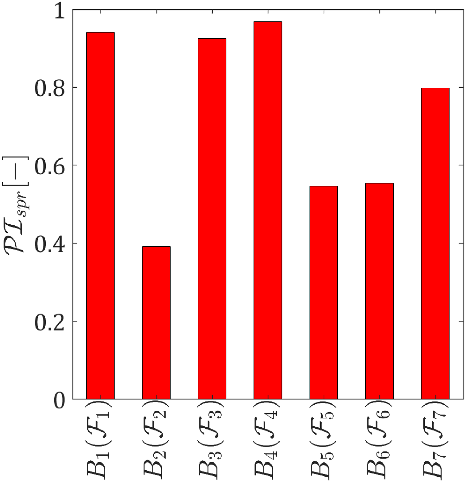
Figure 23 displays the $\mathcal{P}\mathcal{I}$ for different subsystems equipped with the considered burners. It is evident that a considerable difference in the values compared to the FIRC-MC simulations can be seen in some cases. For instance, the $\mathcal{P}\mathcal{I}$ value for burner 2 obtained from FIRC-MC simulations is 0.3912, while according to Figure 17, it is approximately 1.5 times higher. This highlights the strong dependence of the $\mathcal{P}\mathcal{I}$ on the sampling of reflection coefficients. Another noteworthy observation is that the $\mathcal{P}\mathcal{S}$ obtained from SPRRC-MC is consistently lower than that from FIRC-MC, as expected. Because the FIRC-MC simulations are considered the most conservative scenarios and are equivalent to the lumped model in the DCS criterion.

Figure 23.

The probability of instability obtained from the SPRRC-MC simulations.

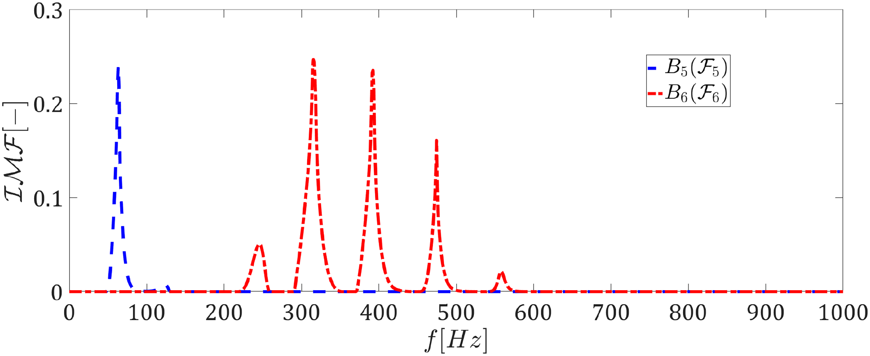
Upon closer examination of Figure 23, it is observed that the SPRRC-MC-based $\mathcal{P}\mathcal{S}$ values for burner 5 and burner 6 are nearly identical. However, when we analyze the $\mathcal{I}\mathcal{M}\mathcal{F}$ over frequency for these two subsystems (see Figure 24), the intuition suggests that burner 5 should exhibit a lower risk of instability across the frequency range. This discrepancy can be attributed to the limitations of the SPRRC-MC simulation, which generates reflection coefficients with limited variations in their frequency dependencies. The conclusion is that the results of statistical analysis of results of MC simulations based on FIRC or SPRRC methods to sample all possible passive acoustic embedding of the burner should be taken with caution, as they may lead to erroneous conclusions. Accordingly, the task is to find a proper method to get representative to the nature method of sampling of functions for the MC simulation of a thermoacoustic appliance is still actual and requires dedicated efforts.

Figure 24.

The instability manifestation fraction versus frequency for only given subsystems equipped with $B_5({\mathcal{F}}_5)$ and $B_6({\mathcal{F}}_6)$ .

In summary, while a definitive and universally applicable figure-of-merit for comparing different burners in thermoacoustic systems has not been identified, this study successfully highlighted the limitations and challenges of existing approaches. The proposed analysis methodology allows us to reveal a possible deficiency of methods relating to MC type of simulations. It is identified that the crux of the problem is related to the difficulty to ensure a proper sampling set of the acoustic embedding of a burner. This aspect and the corresponding pitfalls of the MC approach would be difficult to identify without the help of analysis based on the approach developed above.

So far, the concept of the $\mathcal{I}\mathcal{M}\mathcal{F}$ was introduced, followed by the definition of the thermoacoustic quality factor, $\mathcal{S}$ . Using this factor, multiple thermoacoustic systems in various scenarios were analyzed to rank different burners (or subsystems) based on their risk of instability. Additionally, the proposed thermoacoustic quality factor was compared to two alternative methods, the FIRC-MC and SPRRC-MC simulations, commonly referenced in the literature. This comparison highlighted the limitations of these methods and explained situations where they might lead to incorrect estimations of the thermoacoustic quality of the burners (or subsystems) under consideration. Moving forward, this knowledge will be applied to a lab-scale combustion system for demonstration purposes in the following subsection.

Experimental demonstration of the application of $\mathcal{S}$ factor

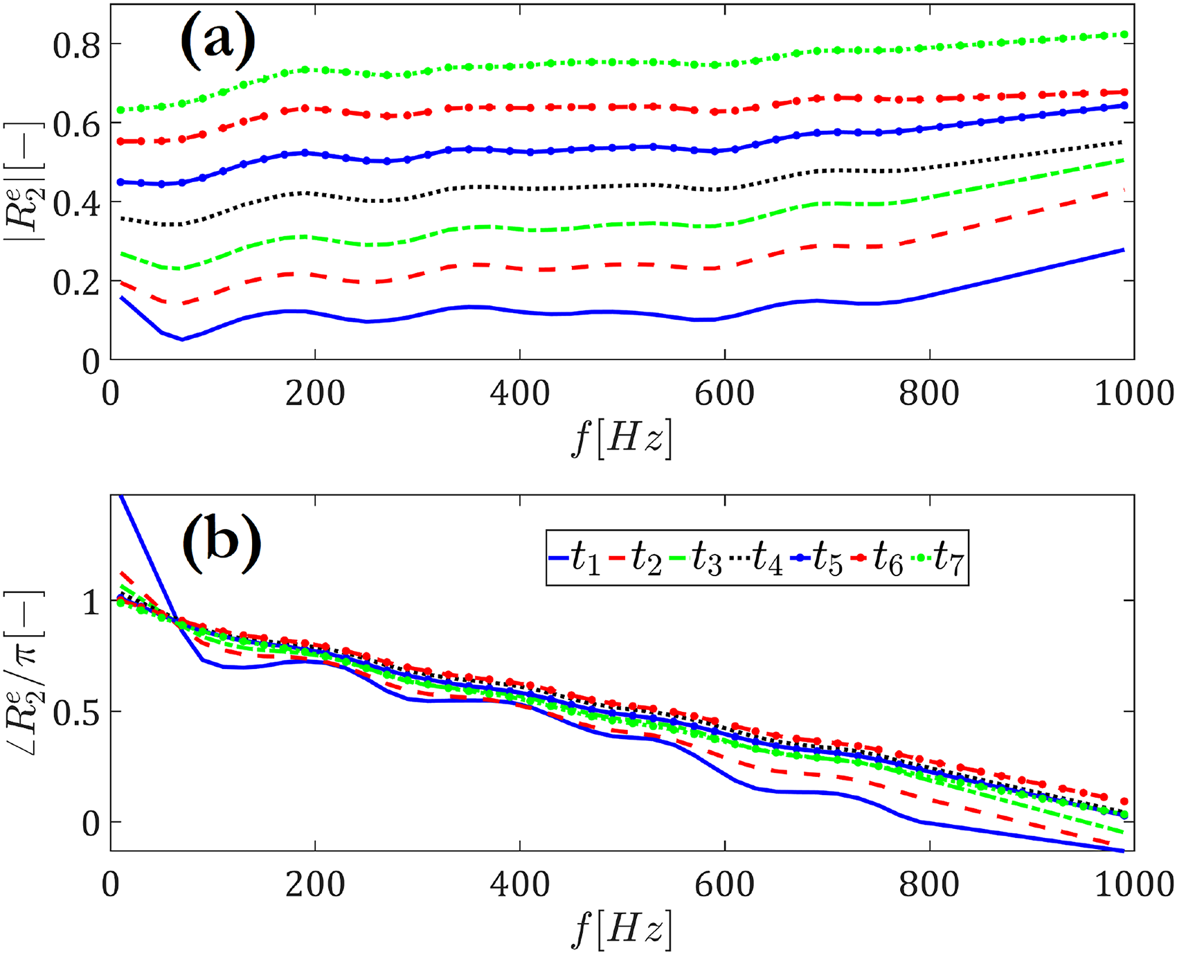
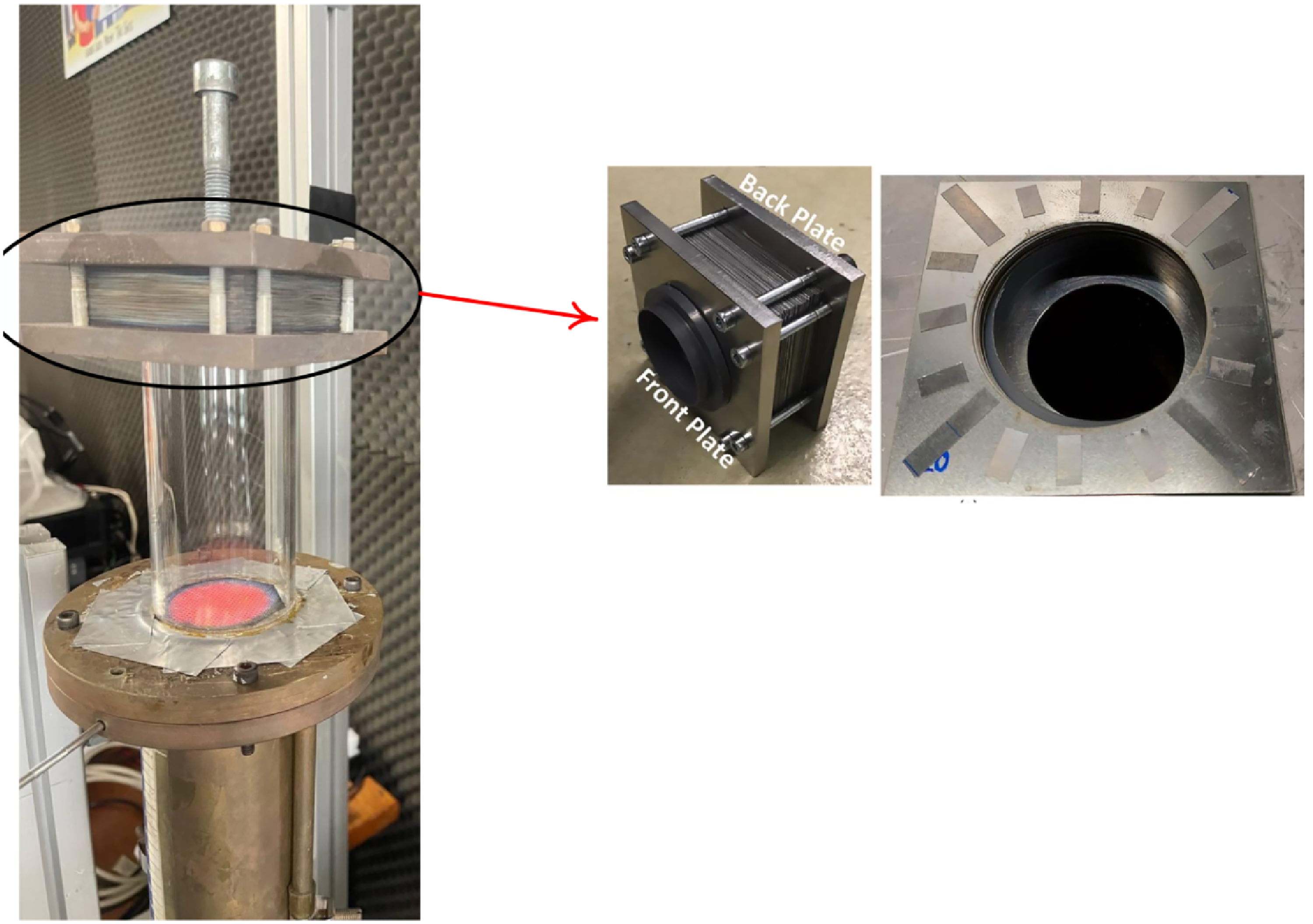
The motivation in this part is to compare the thermoacoustic quality of two different perforated burners made from bulk brass and fibrous SiO₂ plate, as shown in Figure 25, at a thermal power of $P=1.13$  kW and a fuel-to-air ratio of $\varphi =0.8$ . These burners are placed in a combustion system with known upstream acoustics, but with downstream subsystems with unspecified and variable acoustic properties. The configuration of this lab-scale combustion system is presented in Figure 26. As shown, a duct with a length of $L_1=0.84$  m is terminated with a loudspeaker box on the upstream side of the burner. To obtain the total reflection coefficient of the upstream subsystem according to equation (14), the reflection coefficient of the termination, $R_1^e$ , must be known. It can be obtained via a separate reflection coefficient measurement using an impedance tube and the multiple microphone methods (MMM).^22–24 Figure 27 shows the reflection coefficient of the upstream termination across the entire frequency range of interest.

Figure 25.

A view of two considered perforated burner decks in the current section: (a) the burner made from brass with diameter of perforation 3 mm and pitch 6.5 mm; (b) the burner made from SiO₂ with diameter of perforation 0.8 mm and pitch 2 mm.

Figure 26.

A view of experimental setup.

Figure 27.

The reflection coefficient of the loudspeaker box.

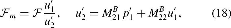
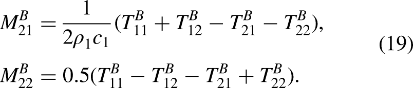
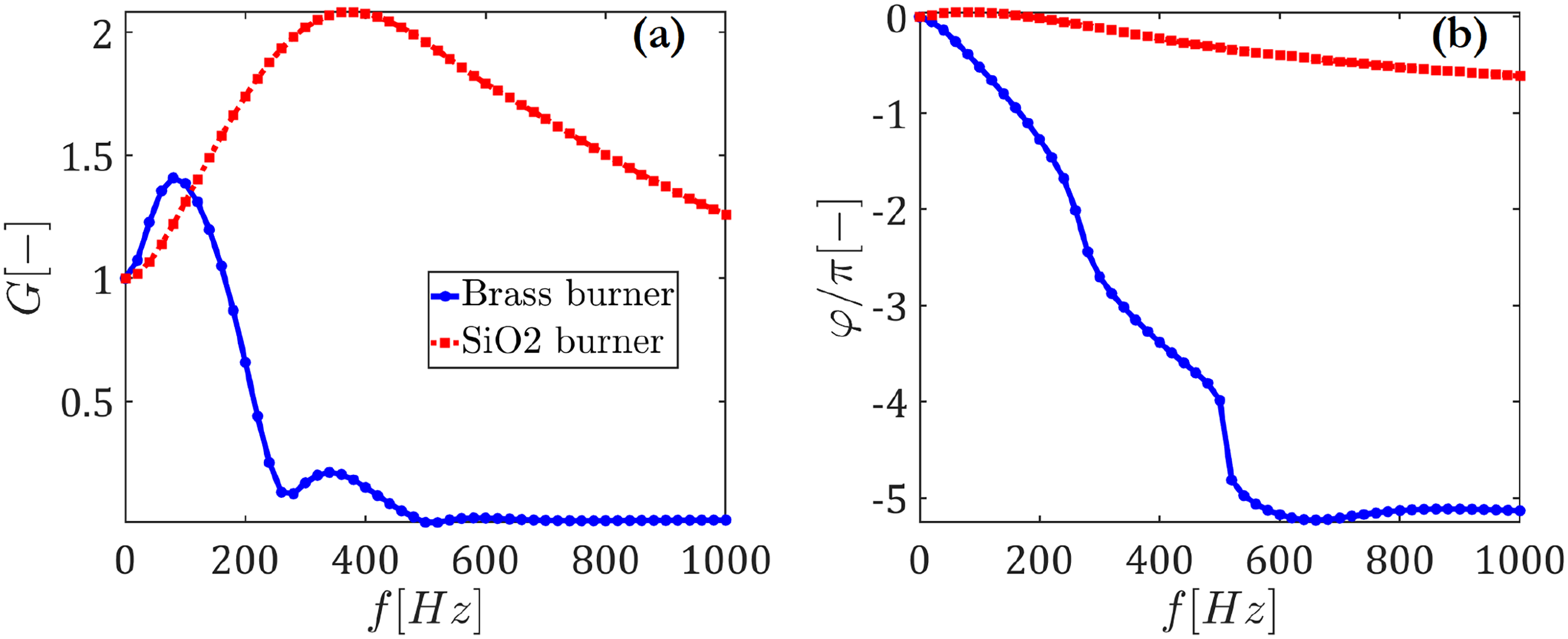
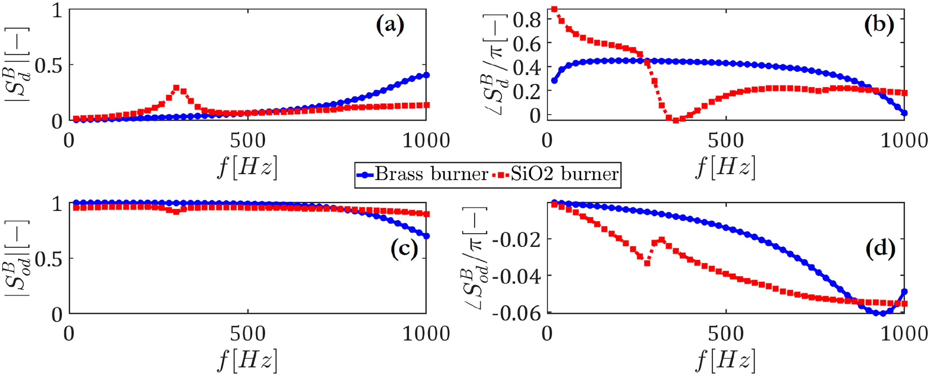
To obtain the stability quality factor, $\mathcal{S}$ , as discussed earlier, the total TM of burners with their corresponding flame must first be determined.^25–27 This can be obtained either using the MMM test of a burner with its corresponding flame together or by separating the burner from its corresponding flame. In the current work, the latter approach is of interest. In this case, the acoustic response of the flame can be characterized by obtaining the flame TF. This is done using the setup shown in Figure 26. The fresh combustible mixture enters the setup from the top of the loudspeaker box, with the burner placed on top, and mounted on a burner holder. On the upstream side of the burner, a constant temperature anemometry probe is positioned to measure the acoustic velocity generated by the loudspeaker. Simultaneously, the fluctuation of the heat-release rate is captured using a photo-multiplier probe equipped with an OH* filter. More details on the construction of the experimental setup can be found here. ²⁰ Figure 28 shows the gain and phase of the flame TFs for both the brass burner and the SiO₂ burner. Additionally, the acoustic properties of the burner are characterized by the absence of the flame but in the presence of a cold/fresh flow. To obtain the transfer/scattering matrix of the burners, the multiple-load SISO reflection tests as explained in Ganji et al. ²⁴ have been utilized. The physical symmetry of the considered perforated burner implies that the diagonal elements of the scattering matrix are identical ( $S_d^B=S_{11}^B=S_{22}^B$ ) and the off-diagonal elements are also identical ( $S_{od}^B=S_{12}^B=S_{21}^B$ ). Therefore, only two independent SISO reflection coefficient tests are required to obtain the two-port scattering matrix of the burners. For brevity, details on the setup configurations, dampers, and so on are omitted. For more information, refer to Ganji et al. ²⁴ Figure 29 shows the diagonal and off-diagonal entries of the scattering matrix for both the brass burner and the ${\text{SiO}}_2$ burner. To form the TM of the burner ${\mathbf{T}}^{\mathbf{B}}$ from the scattering matrix, the expressions read the following:

$$\begin{array}{rl}{T}_{11}^B& =S_{od}^B-\frac{S_d^B{S}_d^B}{S_{od}^B},T_{12}^B=\frac{S_d^B}{S_{od}^B}\\ T_{21}^B& =-\frac{S_d^B}{S_{od}^B},T_{22}^B=\frac{1}{S_{od}^B}\end{array}$$

(17)

Since the TF of the flame, as shown in Figure 28, is based on the measurement of the acoustic velocity at the upstream side of the burner ( $u_1^{\mathrm{\prime }}$ ) rather than at the upstream side of the flame $u_2^{\mathrm{\prime }}$ (i.e. downstream of the burner), the transfer matrix of the burner is used to modify the measured flame TF as follows:

$${\mathcal{F}}_m=\mathcal{F}\frac{u_1^{\mathrm{\prime }}}{u_2^{\mathrm{\prime }}},u_2^{\mathrm{\prime }}=M_{21}^B{p}_1^{\mathrm{\prime }}+M_{22}^B{u}_1^{\mathrm{\prime }}$$

(18)

where $M_{21}^B$ and $M_{22}^B$ are two coefficients that can be defined using the transformation from TM based on $f_{1,2}$ and $g_{1,2}$ Riemann invariants to the TM based on acoustic pressures $p_{1,2}^{\mathrm{\prime }}$ and acoustic velocity $u_{1,2}^{\mathrm{\prime }}$ as

$$\begin{array}{rl}{M}_{21}^B& =\frac{1}{2{\rho }_1{c}_1}(T_{11}^B+T_{12}^B-T_{21}^B-T_{22}^B)\\ M_{22}^B& =0.5(T_{11}^B-T_{12}^B-T_{21}^B+T_{22}^B)\end{array}$$

(19)

By substituting ${\mathcal{F}}_m$ for $\mathcal{F}$ in the R–H jump condition according to equation (5), the TM of the flame ${\mathbf{T}}^{\mathbf{f}}$ can be obtained. Following this, the total TM of the burner with its corresponding flame can be expressed as $\mathbf{T}={\mathbf{T}}^{\mathbf{f}}{\mathbf{T}}^{\mathbf{B}}$ .

Figure 28.

The gain and phase of the flame transfer functions corresponding to the brass and SiO₂ burners.

Figure 29.

The entries of scattering matrix of the brass and SiO₂ burners.

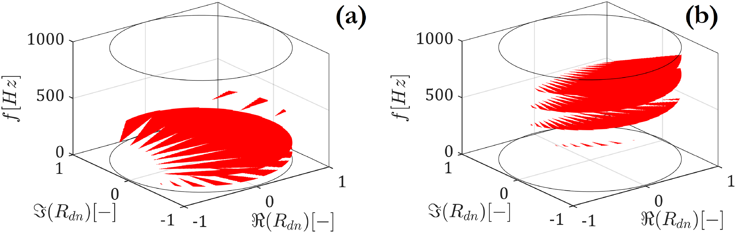
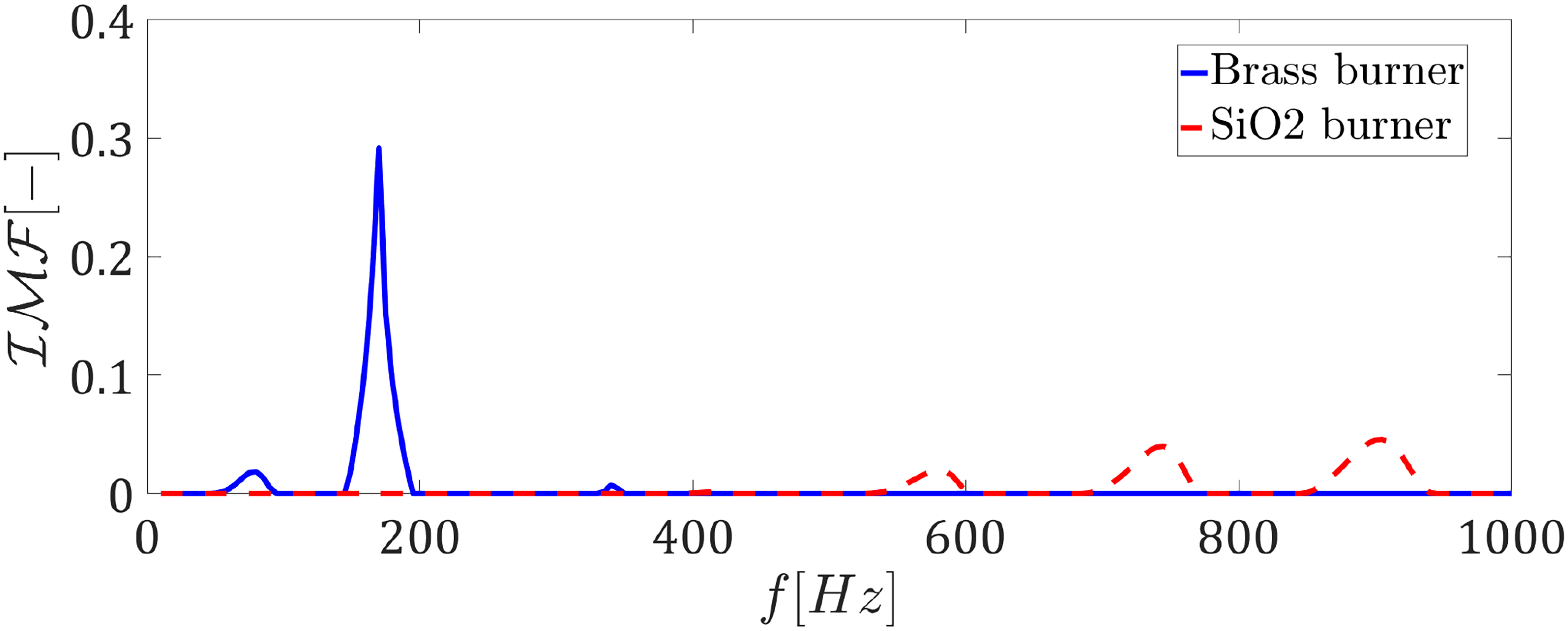
Using the obtained total burner-flame TM and considering the upstream reflection coefficient, the DCS criterion has been employed to construct the stability map across the entire frequency range, as shown in Figure 30. Each slice of the 3D stability maps represents a separate 2D stability map at the specified frequency. These slices are stored sequentially as frames in a video. Refer to “Video-DCS-FOM-BrassBurner” and “Video-DCS-FOM-SiO2Burner” in the supplemental material. Similar to the previous discussions, such as in Figure 10, the $\mathcal{I}\mathcal{M}\mathcal{F}$ diagram for these two burners can be calculated and is presented in Figure 31. For the brass burner, three peak values in its $\mathcal{I}\mathcal{M}\mathcal{F}$ are observed, with the second peak around 200 Hz being significantly dominant compared to the other two. By examining its flame TF, it is clear that this peak corresponds to the −π cross-frequency in the phase diagram, indicating its association with the intrinsic mode. The SiO₂ burner also shows three peak values at higher frequencies, but these peak values are much smaller compared to the highest $\mathcal{I}\mathcal{M}\mathcal{F}$ value for the brass burner. The hump for the SiO₂ burner is slightly wider, while for the brass burner, it is sharper.

Figure 30.

The three-dimensional (3D) stability maps obtained from direct conservative stability criterion of the given subsystem equipped with (a) the brass burner and (b) the SiO₂ burner.

Figure 31.

The instability manifestation fraction versus frequency for subsystems equipped with the brass and SiO₂ burners.

Generally, it is expected that the unstable frequencies of the system will be around the frequencies with higher $\mathcal{I}\mathcal{M}\mathcal{F}$ values. Therefore, for the brass burner, the frequency band around 200 Hz is more critical, whereas, for the SiO₂ burner, all three frequency bands with humps can be considered as possibly unstable frequencies.

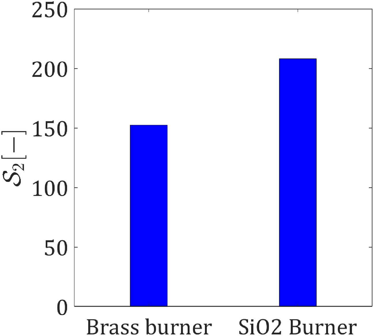
The stability quality factor $\mathcal{S}$ can be calculated to rank different burners globally according to their risk of instability in combination with the considered upstream acoustics. According to Figure 32, the SiO₂ burner, due to its higher value for $\mathcal{S}$ , has a higher chance of operating thermoacoustically stable compared to the brass burner.

Figure 32.

Comparing the thermoacoustic quality of subsystems equipped with the brass and SiO₂ burners using the $\mathcal{S}$ factor.

Now, we design some illustration experiments to check that the finding based on the calculation of $\mathcal{S}$ factor can be reflected when the burners along with the considered upstream acoustic are tested in combination with multiple downstream terminations. To do so, at the downstream of flame, a connecting quartz tube in different lengths has been placed accompanied by multiple downstream terminations with different reflection coefficients as shown in Figure 33. This is good to note that, these terminations have been characterized by the presence of cold flow due to the difficulty of measurement in the presence of hot flow. ²⁴ Although the values of reflection coefficients can be altered due to hot flow, here it is not that significant because the important point is that these terminations should have different values in order to be considered independent tests. The details on the production of these terminations can be found in the work of Saxena et al. ¹⁴ . However, a view of one of these terminations along with a connecting quartz tube can be seen in Figure 34.

Figure 33.

The reflection coefficients of considered terminations for the validation experiments.

Figure 34.

A view of the configuration of the downstream acoustics, with a focus on one of the designed termination and its placement downstream of a burner with its corresponding flame.

By considering an open-end condition as a type of termination denoted by $t_0$ , eight different terminations have been tested along with three different lengths of quartz tubes ( $L_2^{(1)}=5$  cm, $L_2^{(2)}=7$  cm, and $L_2^{(3)}=10$  cm), resulting in a total of 24 different downstream subsystems coupled with the burners. These configurations include their corresponding flames and the upstream reflection coefficient of the load-speaker box, along with the upstream connecting tube. Figure 35 shows a stability map for two burners. The blue circles indicate that the thermoacoustic system equipped with the corresponding duct length and termination operates stably, while the red squares indicate that the system is thermoacoustically unstable for the corresponding downstream duct and termination. By counting the number of unstable statuses (red squares) in the two graphs, one can determine which burner has a higher risk of instability.

According to Figure 35(a), the brass burner with its corresponding flame reveals instability in 19 out of the 24 configurations. Additionally, the unstable frequencies of the unstable system are indicated. A closer look reveals that the reported frequencies are in the range of the critical frequency observed in the $\mathcal{I}\mathcal{M}\mathcal{F}$ diagram (see Figure 31) for the brass burner, as discussed earlier. The dominant unstable frequencies are in the range of the maximum peak in the $\mathcal{I}\mathcal{M}\mathcal{F}$ graph. In the case of the system equipped with downstream duct length $L_2^{(2)}$ and termination denoted by $t_3$ , the system oscillates with two dominant unstable frequencies, with the second frequency nearly double the first. This observation aligns with a peak in the $\mathcal{I}\mathcal{M}\mathcal{F}$ diagram, though it is unclear whether this is due to a period-doubling phenomenon in nonlinear dynamics or a second unstable mode. Further investigation is beyond the scope of the current study. According to Figure 35(b), the SiO₂ burner with its corresponding flame reveals instability in 10 out of the 24 configurations. Clearly, in comparison with the brass burner, the SiO₂ burner shows better thermoacoustic performance, indicating higher thermoacoustic quality. This observation corroborates the findings from the calculation of the $\mathcal{S}$ factor. Additionally, the frequency of instability falls within the range of critical frequencies in the $\mathcal{I}\mathcal{M}\mathcal{F}$ graph in Figure 31.

Figure 35.

The stability map obtained from direct experiments of multiple combustion systems equipped with (a) the brass burner and (b) the SiO₂ burner.

Although the designed experiment clearly confirms the findings from the $\mathcal{S}$ factor in ranking burners based on their risk of instability, it is important to remember that for burners with special flame TFs (e.g. $B_5({\mathcal{F}}_5)$ and $B_6({\mathcal{F}}_6)$ ) according to Table 1, the number and type of terminations can be crucial. To draw reliable conclusions from direct experiments comparing multiple burners, a significant number of different terminations (potentially hundreds) must be designed to ensure that all possible acoustic subsystems are considered. This task is not only nontrivial but also highly demanding. This highlights another advantage of using the stability quality factor $\mathcal{S}$ based on the burner-flame TM rather than relying solely on direct experiments with multiple terminations.

Conclusion

In conclusion, this study has tackled the intricate challenges associated with the evaluation and comparison of thermoacoustic quality in combustion appliance burners. We have introduced a stability quality factor denoted as $\mathcal{S}$ factor, offering a suitable and insightful performance metric. Various burner design scenarios have been meticulously considered presenting a comprehensive understanding of potential concerns within burner/combustor development industries. The incorporation of the $\mathcal{S}$ factor empowers burner developers to establish a robust measure of thermoacoustic quality, complementing other vital quality measures such as emissions, pressure drop, modulation range, and more. In addition, the previously employed MC simulations, coupled with the $\mathcal{P}\mathcal{I}$ as a figure of merit, have been identified as limited and prone to yielding misleading results. In contrast, the utilization of the DCS criterion in the frequency domain has proven insightful, shedding light on the frequency-dependent nature of stability and exposing the limitations of MC simulations relying on FIRC or SPR functions. In the end, the applicability of the proposed quality factor to compare two different types of perforated burner decks has been demonstrated. The experimental validation shows that the predictions match the experimental results very well.

Supplemental Material

Supplemental Material

Supplemental Material