The concept of smart combustion, where nanofuels and electromagnetic interactions are combined to enhance the flame characteristics and improve the control of the combustion process, is introduced as a new paradigm for next-generation hybrid propulsion systems. To gain further insight into the possibility of controlling the fuel location in a turbulent flow, the fundamental case of dispersion of a cloud of charged nanofuel droplets in initially homogeneous and isotropic turbulence under the action of electrostatic fields is investigated. Keeping electrical repulsion forces relatively small compared to the other forces, cases with and without evaporation are studied using direct numerical simulations for different strengths of the external electrostatic field. Results of the non-evaporating cases show that the use of external electrostatic fields enables the control of the location and velocity of the centre of mass of the cloud, with limited effect on the cloud dispersion, which is mainly determined by the background turbulence. Results for evaporating droplets in decaying turbulence show that external electrostatic forces enable a quick separation between cloud and vapour distribution in the case of fast-evaporating droplets. This separation could be further enhanced by designing nanomaterials with specific diffusion properties. This work is the first step towards developing smart combustion and provides new insight into the control of charged nanofuel droplet dynamics under the action of external electrostatic fields.
The development of clean propulsion technologies is a strategic research area to reduce the environmental impact of transportation and allow for a full transition to a zero-pollution society. Elimination of pollutant and carbon emissions is difficult or unfeasible in most fossil-fuelled propulsion systems, even with emission control technology in place.1 Therefore, to improve the emission performance over a wide range of operating conditions, there has been an increased interest in the development and use of alternative fuels as well as on the development of dual-fuel engine configurations.2 Promising alternatives to fossil fuels are the use of tailor-made synthetic fuels3,4 as well as the use of hydrogen.5–7 At the same time, completely new propulsion technologies have also been proposed, such as rotating detonation engines,8 and all electric transportation.9 While industry-scale all electric propulsion is already available for automotive transport, the same is not true for air transportation vehicles with large passenger or cargo capacities to date. One of the main limitations for the transition to full-electric air transportation, especially for long-distance flights, is the low specific energy of currently available rechargeable battery architectures compared to liquid hydrocarbon fuels.10 Similar considerations also apply to energy density, which is higher for hydrocarbon fuels compared to batteries. In the foreseeable future, the energy density of batteries in electric propulsion systems is still expected to remain significantly lower compared to today’s fossil hydrocarbon fuels, thus restricting all electric aircraft (AEA) to small and intermediate scale vehicles.11 Therefore, intermediate solutions such as more electric and hybrid aircraft technologies have quickly emerged among today’s aircraft propulsion research and developments, especially for wide-body aircraft (e.g. see Gnadt et al.11). Hybrid propulsion systems, where the thermal engine is combined with electric units, are the most promising solution for long-distance flights.11 The combination of thermal engines with electric propulsion units allows for a better integration of the propulsion system with the aircraft (therefore, an improved aerodynamics) and at the same time enables the development of distributed propulsion strategies, generally improving the global efficiency of the aircraft propulsion.12 The large availability of electrical energy on board could also offer new possibilities for the control of the combustion process through electromagnetic fields, with the potential of further reducing the emissions and improving the propulsion efficiency. The interaction between flames and low-energy electric fields has been studied extensively, mainly with experiments, in a wide range of configurations, ranging from laminar to turbulent flows, premixed and diffusion flames, AC and DC electric fields (e.g. Park et al.,13 Carleton and Weinberg,14 Marcum and Ganguly,15 Lawton and Weinberg16 and Belhi et al.17). The interaction of the electric field with the charged species generated during the combustion process could lead to a decrease in emissions and changes in shape and location of the flame,18 possibly allowing for the control of flame stability. Furthermore, the energy required to yield significant effects on the flame might be negligible compared to the energy released by the fuel combustion.19 Sakhrieh et al.19 found that 0.1% of the thermal power in a turbulent flame could be sufficient to yield a reduction of 90% in CO emissions. The use of high-energy electromagnetic fields is also currently explored as a new combustion technology usually referred to as plasma-assisted combustion.20–22
Recent combustion research has shown an increased interest in the use of nanomaterials to enhance fuel and flame characteristics. Numerous recent investigations23–25 have reported that the use of nanoparticles in conventional fuels (the so-called nanofuels, i.e., suspensions of nano-sized particles in a base fuel) could improve combustion performance in terms of increased volumetric energy density, enhanced catalytic activity, low ignition delay, higher ignition probability, and reduction of soot and pollutant emissions. Due to the high surface-to-volume ratio, nano-additives provide more contact surface area for rapid oxidation as well as increased catalytic activity or superparamagnetic behaviour,26 depending on the particle material and base fuel characteristics. Synthesis of nanoscale particles has reached a maturity that enables the development of nanomaterials with tailored properties such as surface texture, chemical and electrical properties (e.g.Yao and Zhao27 and Ferrari et al.28). As a consequence, a proper choice of the fuel-nanomaterial combination could allow for tailored physical and chemical properties of the fuel. Catalytic effects of metal oxides or their composites are widely known and used in contemporary devices for emission control in diesel engines.29 Experimental studies with CeO2 and Fe2O3 nanomaterials30,31 provide evidence for enhanced catalytic activity, with also effects on the soot oxidation rates. On the other hand, the partial or full oxidation of nanoparticles could serve as an additional source of heat release due to their high oxidation energy.32 Reduced ignition delay times, an increase in flame stability, significant reduction in CO and unburnt hydrocarbon emissions and possibly a reduction in specific consumption of the base fuel have been observed in previous works on nanofuel combustion.33–35 In particular, non-noble metallic nanoparticles or organic composites such as aluminium and iron oxides, carbon nanotubes and graphene have been investigated in previous works.35 In some cases, it has been shown that improvements of fuel economy can reach 15%–20% with a reduction in pollutant emissions as high as 40%–60%.23 In addition to the direct effect on the reaction process, the presence of nanomaterials also affects the evaporation process. Direct modification of evaporation characteristics due to the presence of suspended nanoparticles in the base liquid has been demonstrated experimentally for nanofluid droplets.36,37 Nanoparticle transport and agglomeration in evaporating liquids can lead to formation of micro-scale structures such as surface shells and densely packed spherical agglomerates.37,38 These structures can subsequently affect heat and mass transfer with the carrier phase. Analytical and numerical models for the prediction of nanofluid evaporation38,39 and particle drying40,37 have been proposed to enable a better prediction of vapour release and formation of the agglomerates. Nanofuel combustion is a flourishing area of research33,41,42 and more investigations are necessary to understand the effect of micro- and nanomaterials on all processes influencing the fuel combustion, from atomisation to evaporation and interaction with turbulence.
The present work is part of a new research direction where the use of nanofuels and low-energy electromagnetic fields is proposed to enhance the combustion characteristics of propulsion systems, possibly leading to improved emission performance in next generation hybrid thermal-electric propulsion configurations. The use of nanomaterials with tailored electromagnetic characteristics is foreseen as one of the main design parameters to augment the interaction between the fuel and electromagnetic fields, leading to the development of a new concept of fuel and combustion design that could be defined as ‘smart combustion’. Figure 1 shows a schematic diagram of the main elements of this new combustion concept and potential routes for the control of the combustion process: (1) control of fuel location; (2) modulation of evaporation properties; (3) direct effects of electromagnetic fields on chemical reactions and species transport; and (4) effects of nanomaterials and their agglomerates on the base fuel chemistry. The control of fuel location is achieved by injecting droplets with a charge and using electromagnetic forces (e.g. generated by an electrostatic field) to modulate their trajectory.43,44 Such droplets could be produced by electrically assisted atomisation (electrosprays). Additional control over the fuel location can be obtained by tailoring the electromagnetic characteristics of the suspended nanoparticles. Note that if the nanofuel behaves as a ferromagnetic material, the droplet trajectory could also be controlled with a magnetic field without the necessity of injecting the droplets with a charge. Evaporation control is achieved by exploiting the porous structures that naturally form during the drying of a nanofuel droplet. A proper design of the nanomaterial could enable the formation of structures with well-defined shape and porosity, therefore allowing to enhance the control over the fuel vapour release. Modulation of the pore size through electromagnetic fields should be explored as a possible mechanism to achieve full control of the fuel release. Modification of the reacting field through the interaction between electromagnetic fields and ions (which could lead to the so-called ionic wind) as well as modification of the chemical pathways45 are further mechanisms to improve the control of the combustion process. Changes in reaction pathways through catalytic effects of nanoparticles and their aggregates as well as heterogeneous combustion are further degrees of freedom offered by smart combustion.46
Schematic diagram of the potential routes to achieve control of the combustion process through the use of nanofuels and electric fields. These include (1) control over the fuel placement, (2) control of vapour release (e.g. through nanoparticle shell formation and electromagnetic modulation as indicated in the inset), and (3, 4) reaction modification (e.g. electromagnetic effects on ion motion, catalytic effects of nanoparticles, and nanoparticle oxidation).
The focus of the present work is on the dispersion and evaporation of charged nanofuel droplets in a turbulent flow under the effect of an external electrostatic field. The control of particle location through electrostatic fields is widely used in a number of technologies. One example is given by electrostatic precipitators.47 Numerical investigations of electrostatic precipitators conducted by Soldati et al.48,49 concluded that the particle collection efficiency strongly depends on the turbulent dispersion, particle drift velocity and particle size. Another example of the potential use of electrostatic fields and charged particles in fluid-based systems is offered by mesoscale combustors10,50 (power generation around 10–100 W; several centimetres in size, see Higuera and Tejera51), where electrosprays are typically used to inject the fuel and electrostatic fields represent an important element for the evolution of the combustion process.52,51 More recently, the control of charged droplets by means of external electrostatic fields has been proposed as new technology to achieve control of fuel mixing and increase the fuel residence time in the vicinity of the injection location.43,44 This adds on previous work where the use of charge injection atomisation was proposed to enhance fuel mixing through a finer control of droplet characteristics and charge-induced secondary break-up.53,54 In addition, it was shown that a sufficiently high droplet charge could also help to control droplet dispersion and avoid the formation of preferential clusters in turbulent flows.55 Electrosprays are also widely used in mass spectrometry applications56 and nanoparticle deposition devices.57 Previous investigations generally demonstrate the potential of electrostatic fields to control the location of charged particles. However, to enable applications in the context of smart combustion, further investigations on the effect of electrostatic actions in a turbulent flow, also considering the effect of evaporation on the droplet dynamics, are still necessary.
To gain knowledge on spray and fuel vapour dispersion under the influence of electrostatic fields, the fundamental case of the dispersion of a cloud of electrically charged nanofuel droplets in a non-reacting turbulent flow is investigated in this work. More specifically, the dispersion of a spherical cloud of charged droplets in homogeneous isotropic turbulence (HIT) under a uniform electrostatic field is studied. The specific objectives of this work are to: (i) evaluate the relative importance of drag and electric forces (including repulsion forces) and provide guidelines for the choice of simulation parameters; (ii) determine the effect of external electrostatic fields on the dispersion of non-evaporating droplets and cloud trajectory; (iii) evaluate the effect of electrostatic forces on droplets dynamics and vapour location for different evaporation time scales and nanofuel characteristics. The study has been conducted using direct numerical simulations (DNSs) in the Eulerian-Lagrangian framework, which have been extensively used to investigate both unladen HIT (e.g. Yeung58 and Eswaran and Pope59) and particle-laden HIT (Wang and Maxey,60 Vreman,61 and Papoutsakis et al.62). DNS studies of turbulent flows with particles in electrostatic fields have been conducted in a few cases, for instance in the numerical investigation of electrostatic precipitators.48 To the authors’ knowledge, this is the first investigation of dispersion of charged nanofuel droplets under the action of electric forces in a configuration starting from HIT conditions.
The structure of this article is as follows. The governing equations for the carrier phase and Lagrangian particles as well as the numerical setup and investigated cases are outlined in the ‘Methods’ section. More insight into the forces acting on the droplet and the rationale used to define the investigated cases is also provided. This is followed by the validation of the baseline framework and assessment of the evaporation model for nanofuel droplets (‘Validation’ section). Results for both non-evaporating and evaporating droplets are discussed in the ‘Results and discussion’ section. A summary of the main findings and conclusions closes the article.
Methods
Direct numerical simulations of the dispersion of charged droplets in homogeneous isotropic turbulence are performed using the Eulerian-Lagrangian approach. In the following, the modelling framework and the main modelling assumptions are discussed. The models for the gas phase and Lagrangian particles are presented, followed by the strategy used to impose and solve electrostatic fields, together with the numerical settings used in the present study. The investigated cases are then discussed in detail with a focus on the selection of the parameters affecting the electrostatic interactions.
Gas phase
In non-evaporating cases, the gas phase (also denoted as carrier phase) is treated as incompressible Newtonian flow, resulting in the continuity equation (bold symbols indicate vectors)
and momentum equation
where is the velocity, is the pressure, is the kinematic viscosity and is the density of the gas. Here, represents the momentum source terms from droplet interaction, and indicates the time. For cases with evaporation, the approach of Russo et al.63 is followed, and the kinematic viscosity and density are assumed constant in all simulations conducted in this work. In these cases, a non-reactive binary gas mixture of air and fuel vapour is considered. It should be noted that a constant fluid density is a reasonable approximation only for small vapour concentrations and moderate changes in gas temperature.64 Therefore, our simulation configuration is chosen appropriately to fulfil these conditions. The transport equation for the fuel vapour in a binary (fuel–air) mixture is expressed as follows:
with being the vapour mass fraction, being the binary diffusion coefficient of vapour in the carrier phase and representing the source term due to evaporation. The mass fraction of the second component (air, treated as a single species in this work) is obtained from . Due to the dilute nature of the liquid phase, the influence of spray evaporation on the gas-phase temperature field is expected to be negligible. This was confirmed by preliminary simulations where an energy equation was solved. Therefore, we treat the system as isothermal in all the simulations discussed in this work.
Droplets
The disperse phase is modelled using the Lagrangian approach. Droplets are numerically treated as material points and the corresponding balances of mass and momentum for each droplet are solved.65 It is assumed that the only forces acting on the -th droplet are the drag due to the interaction with the carrier phase, , and the electrostatic force, , due to the interaction with the electrostatic field. All the other forces, including gravity, Magnus, Basset and Saffman forces, as well as virtual mass, are neglected.65 This allows us to isolate the effects of electrostatic forces and aerodynamic drag. Brownian motion and rotational motion are not considered. The sphere drag correlation introduced by Putnam66 is used to compute the drag force. For the sake of simplicity, it is assumed that the evaporation process has a negligible effect on the drag forces. Therefore, the drag coefficient is computed from a droplet Reynolds number, , based on the bulk gas properties for both non-evaporating and evaporating cases. Note that for evaporating cases, a corrected droplet Reynolds number based on the film properties is often used to consider the effects of evaporation on the drag force.67,68 These effects depend on the fuel type and typically lead to a decrease in the drag coefficient.67 The approximation made in this work allows us to study the cloud dispersion without defining a specific base liquid for the droplets. We anticipate that this approximation will not affect the main conclusions of the work, although a change in the drag force will necessarily require a different electric force to obtain the same terminal velocity of the droplets. A detailed investigation that considers different fuels is left for future studies.
Nanofuel droplet evaporation is modelled following a modified -law behaviour with an imposed nominal evaporation rate . This nominal evaporation rate should be interpreted as the -law evaporation constant of the base liquid fuel in absence of nanoparticles. To take into account the effect of nanoparticles on the evaporation process, the evaporation rate computed for pure liquid droplets is modified following the correction model for nanofluids developed by Wei et al.38 According to Wei et al.,38 it is assumed that during nanofuel droplet evaporation, nanoparticles accumulate at the surface of the droplet (resembling the formation of shells or porous structures), thus decreasing the effective surface area available for evaporation. The droplet evaporation mass flow rate is computed as follows:
where is the droplet mass, is the droplet diameter, is the liquid density and gives the effective evaporation rate in the same fashion as proposed by Wei et al.38
As derived in detail by Wei et al.,38 the nanofluid evaporation correction factor can be expressed as follows:
In equation (5), , with being the nanoparticle contact angle at the droplet surface, defined as the angle between the droplet surface tangent and the nanoparticle tangent.38 and are the initial volume fraction of the nanoparticles in the droplet and initial droplet diameter, respectively. The droplet surface blockage, (originally named E by Vehring et al.69), depends on the nanoparticle Péclet number, , with indicating the diffusion coefficient of the nanoparticles in the liquid, and was analytically derived by Vehring et al.69 to be equal to
where denotes the normalised radial coordinate within the droplet. Accurate numerical integration of the denominator becomes computationally expensive for variable Péclet numbers and large number of droplets. Vehring et al.69 proposed a polynomial approximation valid for . An expression for a wider range of Péclet numbers is used in the present work by making use of two fourth-order polynomials for low and high Péclet number regimes with a relative error of less than 1% for . Note that in this work, the Péclet number is directly imposed rather than being computed from the diffusion coefficient of nanoparticles. The model by Wei et al.38 allows for the prediction of the shell formation, which indicates the end of the first stage of evaporation. After a densely packed shell is formed (indicated by a maximum nanoparticle volume fraction on the droplet surface of 0.6), the diameter of the nanofluid droplet is assumed here to stay constant (terminal diameter) until complete liquid depletion.
We assume a constant nominal evaporation rate and constant nanoparticle throughout each simulation, as in the original nanofuel evaporation model.38 It is worth noting that in the approach adopted here, the evaporation characteristics of the nanofuel (given by the combination of base fuel and nanoparticles) are fully described by , , , and , which in practical applications must be selected based on the specific nanofuel. Note also that the correction of the nominal evaporation rate through the correction factor is performed under the assumption that the main effect of nanoparticles on droplet evaporation lies in the reduction of droplet surface area available for vapour release. In addition, since the -law is used, it is implicitly assumed that mass and heat transfer between the droplet and the carrier phase have already reached an equilibrium, which, in the limit of single-component droplet, implies constant droplet temperature. Therefore, there is no heat-up period and no energy equation is solved for the droplet. The effect of convection on the evaporation rate is also neglected, which is valid in the limit of small droplet Reynolds number. The development of models for nanofuel evaporation is an active field of research (e.g. Sazhin et al.70) and more advanced and comprehensive models should be developed in future studies. The source terms in the gas phase equations from droplet interactions due to drag and mass transfer are computed as presented by Higuera52 by assigning each droplet source term to the finite volume cell where the droplet is located. Carrier phase quantities at droplet positions are linearly interpolated from finite volume cell centres.
Electric properties
The computation of the electric field is conducted in the Eulerian framework. The forces acting on the electrically charged droplets, including the interactions with other charged droplets, are computed from the local electric field. No external magnetic fields are considered. Furthermore, the induced magnetic field due to the motion of charges is assumed to be negligible. A charge-free carrier phase is assumed, meaning that all the charges are confined within the nanofuel droplets. Under the above assumptions, the electrostatic field can be computed by solving the equation for the electrostatic potential , which is expressed by the following elliptic partial differential (Poisson) equation:17,51,71
where is the local charge density in the Eulerian framework and is the vacuum permittivity (the particle-laden gas-phase permittivity is assumed to be equal to ). The electric field, , is directly computed from the gradient of the potential field:
The electric force, , acting on the -th droplet then equals
where is the net charge in the -th droplet and is the individual nanofluid droplet charge density, with being the droplet volume. Following the same strategy used for the computation of the droplet source terms in the gas-phase transport equations, the local charge density, , in equation (7) is computed by considering the charges of all the droplets in a given computational cell. It should be noted that the approach used in this study could lead to inaccurate evaluations of droplet-droplet Coulomb forces, especially in the case of high values of charges and short distances between droplets. To improve the prediction of droplet-droplet interactions, hybrid numerical frameworks have been developed for both non-evaporating72–74 and evaporating75 charged droplets. In such hybrid methods discrete Coulombic droplet-droplet interactions are considered in the near field (where the interactions between droplets are more significant), whereas long-range interactions are computed from the electric field evaluated in the Eulerian framework. Considering the low value of the repulsion forces in all the conditions investigated in this study (see ‘Investigated cases’ section), no specific near-field treatment is adopted. A comparison with the forces evaluated by using the discrete Coulombic method for near-field interactions shows that the approach adopted in this study leads to deviations of the total force acting on a droplet lower than 1% in all investigated cases (analysis performed considering the initial configuration of the droplets).
Note also that the computation of electric forces on a given droplet from the local value of the electrostatic field should not consider the self-induced electrostatic field, which is automatically included by computing in equation (7) from the charges of all droplets. Therefore, in principle, the computation of the force on a droplet should include a correction to eliminate the force contribution due to the self-induced electrostatic field. The value of the correction required in the specific configuration investigated in this work was found negligible (at least four orders of magnitude smaller than the forces due to the external electric field). Furthermore, the droplet charge is assumed to not vary during the evaporation process and turbulent transport (therefore increases with evaporation of the liquid phase). Charge transfer to the gas phase and instability phenomena due to the presence of charges, such as Coulomb explosions,51,72 are neglected. In addition, possible fragmentation of solid structures due to repulsion between nanoparticles is also neglected. The charge distribution and evolution depend on many factors, including external electric field and electromagnetic properties of liquid and nanomaterial, and should be the focus of future research. The assumptions made in this work allow us to simplify the scenario and provide a first assessment of the interactions between electric and drag forces acting on charged nanofuel droplets.
Configuration and numerics
As schematically shown in Figure 2, a box domain with cube length is considered. A spherical cloud of droplets is initially placed at the centre of the domain, with droplet positions randomly distributed within the cloud. Periodic boundary conditions are imposed for all flow quantities in the Eulerian framework. A non-periodic external potential difference is imposed by two virtual electrodes located at two opposed boundaries of the box domain, as indicated in Figure 2. Such a potential difference generates an external electrostatic field aligned with the -axis. The electric potential, equation (7), is solved on a second mesh with the potential imposed at the electrodes and zero-gradient boundary conditions imposed on the remaining four boundary patches. The computational meshes of both domains are kept equal in this study, resulting in a direct mapping of electric quantities onto the gas-phase domain. Simulations performed in this work are intended to represent a single droplet cloud dispersion in homogeneous turbulence, rather than a uniform array of interacting clouds. Therefore, periodic boundaries are not used for droplets, which are removed as they reach a boundary face. This is in contrast with previous particle-laden DNS with electric fields where both fully periodic and quasi-periodic76–78 boundary conditions were explored. It should be noted that the approach used in the present work limits the analysis to the time span prior to droplets or vapour reaching the domain boundaries. Several ‘numerical experiments’ are required for each configuration to collect enough data for statistically converged results due to the short dispersion times and constraints on the initial number of droplets (see ‘Investigated cases’ section). A convergence study based on the ensemble average of the first four statistical moments of flow and droplet velocities was conducted to determine the number of trials required per configuration. The mean value and one-sided Student-t confidence intervals (see Overholt and Pope79) with a 90% confidence were used to quantify statistical convergence of the ensemble averaged moments. As a result, six trials per configuration were found sufficient to achieve statistical convergence of the ensemble average of flow field and particle quantities. Therefore, six simulations with initial flow fields extracted from uncorrelated timesteps of the statistically stationary unladen flow were performed for each configuration and condition discussed in the following. At the same time, a minimum number of 1000 droplets per simulation trial was found to be necessary to achieve convergence of droplet cloud statistics.
Periodic box domain with spherical droplet cloud at initial time.
Both decaying and ‘stationary’ (in the limit of negligible effects from droplets) HIT simulations are performed in this work. Stationary turbulence is obtained by means of a low wavenumber stochastic forcing algorithm based on an Ornstein-Uhlenbeck process,80,81 similar to the forcing processes used in previous studies.59–61,82 The finite-difference formulation of the stochastic differential equation for the spectral force contribution for discrete wavenumbers at time step is given by The first term on the right-hand side represents the force history accounting for convergence towards a mean value. corresponds to a random contribution from a Wiener process scaled by a scalar factor . The control terms and determine the temporal development and converged statistics of the process and subsequently the overall level of turbulence. The discrete wavenumber contributions are transformed to the physical space using a inverse discrete Fourier transform (DFT) algorithm (). The right-hand side of equation (2) is extended by the forcing vector source term where and denote the real and imaginary part of the inverse-transformed forcing vector . Forcing is conducted in a limited band of small wavenumbers. A range of 80 whole wavenumbers () in each Cartesian direction was found to be suitable in the HIT configuration by specifying a forcing wavenumber interval of as proposed by Wang and Maxey.60 The numerical properties used in this work are given in Table 1 (case OF), together with the corresponding parameters from a reference study60 (case WM) used for validation (see ‘Validation’ section). The number of finite volume cells in each Cartesian direction is denoted by . The forcing parameters were chosen to be , , and .
HIT: homogeneous isotropic turbulence; WM: Wang and Maxey; OF: OpenFOAM (present work); CFL: Courant–Friedrichs–Lewy.
Simulations were performed using OpenFOAM-v7. A new Euler-Lagrangian DNS solver was developed to include Lagrangian particles as well as electrostatic fields and their mutual interactions starting from the base DNS solver already available in OpenFOAM. Pressure–velocity coupling in the incompressible flow field is achieved with a PISO (pressure-implicit with splitting of operators) algorithm.83–85 The unstructured nature of the OpenFOAM framework restricts spatial discretization schemes to rather low-order accuracy compared to structured codes where 10th-order spatial schemes are not uncommon (see e.g. Borghesi et al.86). In this work, a second-order accurate cubic differencing scheme87 is used for diffusion terms. Advective transport is treated with a second-order accurate central differencing scheme. A second-order implicit scheme (see Zirwes et al.,87 Jasak,88 and Vo et al.89) is used for temporal discretization. As proposed by Pope,81 a is desirable for DNS codes. However, various authors60,61 have successfully applied higher numbers in their DNS studies. A volume average CFL () equal to 0.1 is used in this work with in the entire domain. The Lagrangian particle momentum equation is integrated with first-order accurate implicit schemes. Four particle sub-integration steps are performed per timestep in order to improve the accuracy of the computation of droplet quantities. The Poisson equation for the electrostatic field is solved using a second-order linear spatial scheme. The computation of the flow field, droplet dynamics and electrostatic field is done using a segregated approach. For each time integration step, the electric potential and related electric field are computed first. Then, the flow field equations are solved followed by the Lagrangian droplet equations.
Investigated cases
The cases simulated in this study are designed to investigate the relative effect of turbulence and drift imposed by the external electrostatic forces on the differential dispersion of the droplet cloud and fuel vapour. First, simulations in stationary turbulence are performed for non-evaporating droplets. These simulations allow us to maintain a constant level of turbulence and provide a measure of the dispersion of the droplet cloud for fixed turbulence characteristics, a fixed size of the droplets and different strengths of the electric forces. The investigated conditions are meant to represent droplets in a cold flow at atmospheric pressure, such that the assumption of negligible evaporation is consistent with the physical conditions. Then, simulations in decaying turbulence are performed for both non-evaporating and evaporating droplets. These cases are used to investigate the differential dispersion of droplets and fuel vapour for different rates of evaporation and different strengths of the external electrostatic field. The investigated condition represents pre-heated air at atmospheric pressure. The use of a decaying turbulence allows us to better isolate the differential dispersion of fuel vapour and droplets without the additional complexity introduced by the turbulence forcing mechanism.
An overview of the configuration parameters and investigated conditions for non-evaporating droplets in stationary turbulence is given in Table 2. The Taylor Reynolds number, , of the turbulent field is given in Table 4. The initial droplet diameter, (constant for cases with no evaporation), is taken significantly smaller than the Kolmogorov length scale, , of the unladen turbulent flow (). The initial droplet diameter is also small compared to the finite volume cell dimension (). The initial velocity of the droplets is assumed to be equal to zero, with a droplet Stokes number equal to , where and are the droplet relaxation time and Kolmogorov time scale, respectively. The droplet-carrier phase density ratio, , is representative of a typical fuel droplet in cold air at atmospheric pressure. The initial radius of the droplet cloud is taken equal to in all simulations, with an initial droplet volume fraction (corresponding to a number of droplets equal to 2000). The droplet charge and external base potential are expressed in Table 2 by means of non-dimensional droplet charge density and potential difference groups defined as and , respectively, where indicates the RMS of the velocity fluctuations, is the initial droplet charge density (constant in case of no evaporation) and is the base external electric potential difference. For simulations in stationary turbulence, the eddy-turnover time (see Wang and Maxey60) is used as a reference time scale.
Overview of nondimensional parameters for the simulation of the dispersion of a non-evaporating droplet cloud in a homogeneous and isotropic turbulence box (stationary turbulence).
Parameter
Symbol
Value
No. of trials per config.
6
Droplet cloud radius
1/8
Init. droplet vol. frac.
Droplet diameter
Liquid–gas density ratio
627
Droplet Stokes number
St
0.10
Nondim. charge group
11,800
Nondim. potential group
4.12
External pot. difference
0; 0.5; 1; 2
Overview of nondimensional parameters for the simulation of the dispersion of an evaporating nanofluid droplet cloud in decaying turbulence.
Parameter
Symbol
Value
No. of trials per config.
6
Droplet cloud radius
1/8
Init. droplet vol. frac.
Initial diameter
Liquid–gas density ratio
1312
Solid–liquid density ratio
6.69
Nominal droplet lifetime
0.14; 0.28; 0.56
Nanop. Péclet number
Pe
50; 200
Init. droplet Stokes num.
St
0.24
Init. nanop. vol. frac.
0.0016
Nanop. contact angle
40
Nondim. charge group
16,600
Nondim. potential group
5.90
External pot. difference
0; 2
Overview of time-averaged turbulence statistics in the unladen HIT. The present results are indicated by OF, wheres data for comparison, indicated by WM, are taken from the work by Wang and Maxey.60
HIT: homogeneous isotropic turbulence; WM: Wang and Maxey; OF: OpenFOAM (present work); CFL: Courant–Friedrichs–Lewy.
Compared to simulations in stationary turbulence, simulations in decaying turbulence are performed with a higher value of the liquid–gas density ratio, , to replicate the density ratio of typical hydrocarbon fuels in pre-heated air at K and atmospheric pressure. The initial droplet diameter is equal to the one used for non-evaporating droplets whereas the initial droplet Stokes number is equal to 0.24. The density of the nanoparticles is assumed to be , with a liquid–solid contact angle of degrees. The latter is an important parameter for the behaviour of the nanomaterial at the droplet interface and affects the computation of the correction factor of the evaporation rate (see equation (5)). The value of depends on the characteristics of the liquid and nanomaterial and specific values are rare in the literature. Here, the value used by Wei et al.38 for aluminium oxide is adopted. More experimental insights should be gathered to find appropriate values of nanoparticle contact angles for each specific liquid-nanoparticle suspension. Two different nanoparticle Péclet numbers, and , are investigated, which are representative of typical nanofuels.36,38 The evaporation rate used in the simulations is defined by means of the non-dimensional nominal droplet lifetime , with evaluated using the nominal evaporation rate constant, that is, . Here, is the characteristic timescale of decaying turbulence, ( and are the turbulent kinetic energy and dissipation rate, respectively), determined at the time of droplet injection, that is, . Three different evaporation rates and a non-evaporating case are investigated. The initial droplet volume fraction, , is taken equal to , as in the simulations with stationary turbulence. This relatively low value of allows us to reduce the effects of droplets on the gas phase and to keep the fuel vapour mass fraction low when evaporation is activated. A low fuel vapour mass fraction is an important requirement for the constant density approximation used in this study. Parameters used in the simulation of evaporating nanofuel droplets are summarised in Table 3. The initial turbulent profiles for the decaying turbulence simulations are the same as used in the forced turbulence simulations. For cases with decaying turbulence, normalisation in time is performed using the characteristic timescale of decaying turbulence, .
The choice of droplet charge density and potential difference requires particular attention since it determines the external electrostatic force applied to each individual droplet (see equation (9)). In this numerical study, the value of droplet charges is kept low to make the repulsion force between droplets relatively small compared to the other contributions. This allows us to isolate the droplet dynamics due to the sole action of drag forces and externally imposed electric forces. By fixing the initial size of the droplet , the cloud size , and the volume fraction of the droplets , it is possible to analytically compute the number of droplets in the cloud. By imposing the droplet charge density, the electrostatic force for each value of the electric field (potential difference) can be computed. Once the value of the electric charge of the droplets is fixed, it is also possible to estimate the repulsion force experienced by each droplet, which is maximum for s, when the size of the cloud is minimal. Figure 3 summarises the values of external electrostatic force and estimated repulsion force for various values of the nondimensional external potential difference and nondimensional droplet charge density at fixed droplet diameter. Lines at constant value of the external potential difference and constant value of droplet charge density are reported. The forces are expressed in nondimensional form by means of the initial drag force from Stokes’ drag, , acting on the droplets, estimated from the initial level of turbulence . Since the diameter of the cloud, the droplet size and are fixed, the number of droplets considered in Figure 3 is constant. Therefore, for each value of a constant value of is found. If a constant external electrostatic field is imposed, an increase in requires a higher droplet charge density, which implies an increase in .
Mean normalised droplet repulsion force in the cloud against external electric force for , and . Iso-lines at constant nondimensional electric field strength () and constant nondimensional charge density () are shown. The red marker represents the initial conditions used in this work for the non-evaporating case in stationary turbulence at .
Once the value (and, therefore, for a given size of the droplets, initial turbulence level and gas-phase properties) is fixed, the strength of the electrostatic field determines the initial ratio between external electrostatic forces and drag forces, . When this ratio is far greater than unity, the droplets are accelerated towards the direction of the electric field with the forces due to the drag induced by turbulent fluctuations having a minor role in the droplet dynamics. The other extreme is given by values . In this case, the external electric forces are very weak compared to turbulence interaction and the motion of the droplets is mainly dictated by the turbulent structures. A more interesting operating condition is when the value of the ratio between the electric force and drag forces associated to the initial turbulence intensity approaches unity. This scenario allows us to investigate the competing actions of electric drift and turbulent fluctuations on the cloud dispersion. In this work, a value of (indicated in Figure 3 by the triangular marker) is adopted for the base case in stationary turbulence. It is worth remembering that the value of the drag force is only an estimate from the initial level of turbulence, assuming zero velocity of the droplets. Depending on the instantaneous location of the droplets and their relative velocity, will considerably vary during a simulation.
Similar plots can be produced by fixing the ratio and letting the droplet diameter vary. Figure 4 shows as a function of the magnitude of the nondimensional external potential difference, for several values of and droplet charge density group . (the value used in this work for the base case in stationary turbulence) is imposed together with the values of cloud size and initial droplet volume fraction used in the present work. The minimum droplet size shown corresponds to the (arbitrarily chosen) limit of droplets in the cloud. For every value of the droplet diameter it is possible to find a combination of droplet charge density and external electric field to keep repulsion forces low. The operating condition used in this work for the stationary turbulence simulations (non-evaporating droplets) is indicated in Figure 4 by a triangular marker. It should be noted that the dimensional quantities corresponding to the operating condition could result in a relatively high electric field (above the break-down threshold in air – ideal value between parallel electrodes around 3 MV/m in air at atmospheric conditions90). To decrease the value of the electric field for a given value of the external electrostatic force and, at the same time, keep the repulsion force between droplets small, lower initial droplet volume fractions are required. Note that once the electrostatic force is fixed, the charge density is inversely proportional to the electrostatic field for a given geometrical configuration. It might be interesting to look at configurations with high droplet charges and lower electric fields in future works by investigating cases where repulsion forces are not negligible.
Droplet repulsion-drag force ratio for the present level of turbulence and assuming and . Iso-lines are shown for constant () and constant (). Data points are shown for a volume fraction of . The marker represents the initial conditions used in this work for the non-evaporating case in stationary turbulence at .
To evaluate the effect of the external electric field on the dynamics of the cloud, simulations with different values of the external potential difference are performed. For non-evaporating droplets in stationary turbulence, four different values of the external potential difference are investigated, that is, , , , and (see Table 2). For cases in decaying turbulence, we only consider no and strong external electrostatic fields (), as shown in Table 3. Simulations with zero potential difference are used as reference case and have been performed with no electric charges. A preliminary simulation with zero external potential and fixed droplet charge density (same value as used in all the other configurations) showed small cloud repulsion effects, confirming the suitability of the setup to reach negligible effects of droplet repulsion on the cloud dynamics. All simulations with electric fields were carried out at the same initial droplet charge density (with droplets assumed to be negatively charged).
Validation
Unladen HIT flow
Validation of the capability of the solver used in this work to predict the underlying turbulent flow was performed by comparing the unladen stationary turbulence simulation against the DNS results from Wang and Maxey,60 which were conducted at a similar Taylor Reynolds number (). As indicated by previous studies with OpenFOAM89,85 and other finite volume codes (e.g. Vreman61), a higher spatial and temporal resolution is required for the finite volume formulation with low-order discretization schemes to obtain resolved spectra. Preliminary simulations conducted with the same spatial resolution of Wang and Maxey60 confirmed these observations, as the reference energy spectra could not be reproduced at large wavenumbers with sufficient accuracy. Good resolution of the spectra for the case under investigation was obtained for wavenumbers which corresponds to a double resolution in each spatial direction compared to the work conducted with a spectral code.60
Statistical convergence of the flow is reached around . Averaging in space and time is performed for another 90 eddy turn-over times after reaching statistical convergence. Table 4 shows a comparison between the present results (case OF) and the reference DNS by Wang and Maxey60 (case WM) in terms of turbulence statistics. The number of cells used to discretize each direction is denoted by . The averaged one-dimensional energy spectrum is given in Figure 5. The energy spectrum is normalised by the Kolmogorov scales. Only one spatial direction is displayed in the spectra due to flow isotropy (also verified by comparing two-point correlation of all velocity components – not shown here). Seven orders of magnitude of energy are resolved in the energy spectrum with a strictly monotonic decrease in energy towards the smaller length scales. The energy predicted in the present work is slightly overestimated for large wavenumbers compared to the reference DNS.60 Overall, the unladen HIT simulation of the present work gives a well-resolved range of turbulent scales making the numerical framework suitable for DNS despite the requirement of an increased spatial resolution due to the use of relatively low-order discretization schemes.
Unladen box turbulence direct numerical simulation one-dimensional (DNS 1D) energy spectrum from the present work () compared with results from the work by Wang and Maxey60 ().
Nanofluid evaporation model
The nanofluid evaporation model implementation was evaluated against the results from the work by Wei et al.38 Three cases have been simulated, each of them characterised by a constant value of the nominal evaporation rate constant, , and nanoparticle Péclet number. The conditions are summarised in Table 5 for three configurations (cases A to C). Results are shown in Figure 6. The predicted droplet diameter at the end of the first evaporation stage (when reaches the minimum value) is equivalent to the reference values for the various cases. The time evolution of the droplet diameter is also similar to the results reported by Wei et al.,38 therefore, confirming the reliability of the model implementation.
Validation of the implementation of the nanofluid evaporation model by Wei et al.38: evolution of the droplet diameter for the cases reported in Table 5. The present results are indicated by OF, whereas data from Wei et al.38 are indicated by Wei.
Cases used for validation of the implementation of the nanofluid evaporation model by Wei et al.38
Parameter
Value
Unit
Contact angle,
40
deg
Evaporation rate,
Case A:
m2/s
Case B:
m2/s
Case C:
m2/s
Nanop. Péclet number,
Case A: 1
–
Case B: 3
–
Case C: 25
–
Results and discussion
Non-evaporating droplets in stationary turbulence
The action of electrostatic forces on the dispersion of non-evaporating droplets under stationary turbulence conditions is discussed first. The initially spherical droplet cloud disperses irreversibly and non-uniformly due to the turbulent nature of the flow. As mentioned in the methods section, we recall that droplets are removed from the computation as they reach the domain boundaries. If droplets were not removed, the cloud would eventually distribute over the entire domain, potentially forming regions of preferential droplet concentrations as observed in previous works, for example, Wang and Maxey.60 No such investigations were conducted in this work as the focus is on the dispersion of an individual cloud. Figure 7 shows the evolution of the total number of droplets in the domain for the four values of external potential difference. Only the individual simulation trial out of six with the shortest droplet time-to-boundary is reported for each case. The deviations observed among the trials at the same electric field strength are generally small. Droplets start to leave the domain around for all . In general, the time-to-boundary is short compared to the turbulent time scales for all four cases. Approximately seven Kolmogorov time scales are captured before the first droplet reaches the boundary. The temporal evolution of the one-dimensional turbulence energy spectrum computed considering the entire domain in the absence of an electric field, , is shown in Figure 8. Perturbations of the energy spectrum due to the droplet motion are mostly negligible. A small temporary increase in energy at the small scales, that is, at large wavenumbers, is observed at . This may be caused by the relatively large initial relative velocity between the droplets and the flow as droplets are initialised with zero velocity. This effect vanishes at later times as the droplets tend to follow the flow with small relative velocity. It should be noted that modification of the turbulent carrier flow due to the droplets can only be studied to a limited extent for two-way coupled droplets with turbulence forcing.91,92 Following the recommendations by Lucci et al.,93 a detailed analysis of the spectrum modulation compared to the unladen flow is not conducted here to avoid misleading interpretations due to overlap effects of the stochastic turbulence forcing and particle two-way coupling.93
Time evolution of the normalised number of droplets in the domain as a function of time in stationary turbulence simulations with non-evaporating droplets for various electrostatic field strengths, (), (), () and ().
Temporal evolution of the energy spectrum for non-evaporating droplet-laden flow in stationary turbulence with .
The plane-averaged volume fraction of droplets (average performed in planes normal to the direction of the external electrostatic field, i.e., normal to the -axis) as a function of time and distance from the centre of the box, is shown in Figure 9. Results for the two extreme values of investigated in this work are reported. The dispersion of droplets without external electrostatic field is isotropic in space and increases in time. When an electric potential difference is imposed, a preferential shift of the charged droplets in the direction of the external electrostatic field is observed.
Plane-average of the droplet volume fraction (average performed in planes normal to the direction of the external electrostatic field, i.e. the -axis) as a function of time and for non-evaporating clouds in stationary turbulence without (top) and with (bottom) external electrostatic fields.
Figure 10 shows the time evolution of the normalised location of the cloud centre of mass along and normalised standard deviation of the droplet locations along , defined as , as a function of time. Here, denotes the number of droplets in the system. An additional configuration with zero external potential and charged droplets was also run to quantify the effect of repulsion forces in the absence of external electrostatic fields. A preferential motion of the cloud in the direction of the external electrostatic field is observed when a potential difference is applied. The cloud moves faster with increasing external potential difference as a consequence of the larger electrostatic forces. Note that in the case , a small motion of the cloud centre of mass, equal to about 2% of the box side , is observed. This motion is due to the limited number of trials used to compute averages and should tend to zero for an even larger number of trials. Nevertheless, the simulations clearly show the effect of increasing potential difference on the cloud dynamics. The spatial dispersion of the cloud relative to the cloud centre of mass increases with time, as indicated by the time evolution of . All investigated cases show a similar dispersion behaviour, suggesting that electric forces simply translate the cloud without altering the dispersion process, which is mainly determined by the underlying turbulence. The comparison between simulations at with and without droplet charges shows similar behaviour in terms of the trajectory of the cloud centre of mass and cloud dispersion. These results demonstrate that in the investigated cases, repulsion forces are very small and, therefore, have a negligible effect on the statistics of the cloud motion.
Normalised location of the cloud centre of mass (left) and st. dev. of droplet positions (right) in the direction of the external electrostatic field in the case of non-evaporating droplets in stationary turbulence for (), (), () and (). Square markers () represent the droplet centre of mass and from simulations at with charged droplets.
A detailed overview of droplet force magnitudes (drag and electric forces) is shown in Figure 11 for and . Results for different strengths of the external electric field are shown together with cases at with and without charged droplets. The electric field generated by the charged droplets used to evaluate droplet repulsion forces, , is computed as . Repulsion forces are low compared to drag and external electrostatic forces in all investigated cases. Droplet drag forces decrease in time compared to the initial condition as the droplets tend to follow the turbulent flow with small relative velocity (small Stokes number of the droplets). In cases with an external electric field, a force balance between drag and electrostatic forces is reached for .
Budget of average magnitude of drag and electrostatic forces (normalised by the initial mean drag due to turbulence) acting on droplets at (left) and (right) for non-evaporating droplets in stationary turbulence. Drag forces, (black), electrostatic forces, (red), and inter-droplet repulsion forces, (green, not visible with this scale due to low force magnitude), are shown. Cases at with and without charges in the droplets are reported to investigate the effect of repulsion forces.
The absolute values of the components of drag force and electrostatic force acting on the cloud, both parallel to the direction of the external electric field, are compared in Figure 12. These forces are opposed in their direction of action and increase with increasing external potential difference. Drag and electrostatic forces show similar magnitudes for each value of the external potential difference. The (arithmetic) mean droplet Reynolds number is also shown in Figure 12. An increase in Reynolds number indicates an increase in the relative velocity between the droplets and the carrier phase until a balance between drag and electrostatic forces is reached. Once equilibrium is reached, the cloud moves with a constant average terminal velocity which depends on the external electrostatic field as well as on the droplet diameter and gas properties. Note that in this condition, with reference to Figure 11 right, the drag force induced by the presence of an external electrostatic field is higher compared to the drag force resulting from the sole turbulent fluctuations (case with no external electrostatic field). In other words, electrostatic forces are relatively high compared to the drag induced by the background turbulent fluctuations (for time instants sufficiently far from the initial state) in all the cases investigated in this work. The probability density functions (PDFs) of the magnitude of the drag force acting on the droplet and the droplet Reynolds number at are depicted in Figure 12, right. An increase in the mean with increasing strength of the electrostatic field is observed, as an effect of the drift of droplets induced by the electric forces. At the same time, the width of the distribution is only moderately affected by an increase in external potential difference, consistent with the negligible effects of the external electrostatic forces on the cloud dispersion observed with reference to Figure 10.
Temporal evolution and distribution of forces acting on the droplets and droplet Reynolds number for different strengths of the external electrostatic field in the case of non-evaporating droplets in stationary turbulence. From left to right: absolute values of the average drag (black) and electric force (red) components in the direction of the external electric field as a function of time; time evolution of the average droplet Reynolds number; probability density function of the magnitude of the drag force acting on droplets at ; probability density function of at . The data is shown for various electrostatic field strengths, (), (), () and ().
Nanofuel droplets in decaying turbulence
All simulations with evaporating droplets have been performed with decaying turbulence. The initial droplet volume fraction of leads to dilute vapour concentrations (), which justifies the incompressible DNS formulation used in the present investigation. The turbulent kinetic energy, , and dissipation rate, , at are shown in Figure 13. Similar results (not shown here) were also found for cases with , which shows that the particle perturbations induced by the external electrostatic force have a negligible effect on large-scale turbulence statistics for the conditions investigated here.
Temporal evolution of turbulent kinetic energy, , and dissipation rate, , at (decaying turbulence).
The mean droplet motion and the cloud dispersion in the direction of the external electrostatic field are shown in Figure 14 by means of the location of the cloud centre of mass and normalised standard deviation of the droplet locations along (), respectively. Results from simulations with different droplet evaporation timescales, , are reported. Note that with no external electric fields, cases with different evaporation rate show very similar behaviour, therefore, only one case is reported in Figure 14. For comparison, results from simulations with non-evaporating droplets, that is, , are also shown in Figure 14 (see markers). The application of an external electrostatic field results in a preferential motion of the cloud centre of mass in the direction of the external field. This is consistent with our observations in the simulations with stationary turbulence without evaporation (see Figure 10). The mean motion of the cloud along decreases with increasing evaporation time. On the contrary, the cloud dispersion is not affected by the strong electric field and is mainly driven by the turbulent flow. No significant effects of the evaporation time on the cloud dispersion are also observed. Note that the mean motion of non-evaporating droplets under an external electric field (case at ) follows the trend observed for evaporating droplets with increasing evaporation timescale.
Location of the cloud centre of mass (left) and st. dev. of droplet positions (right) in the direction of the external field for , (), , (), , () and , () at in decaying turbulence. Quantities are only shown up to the point of the first droplet leaving the domain. Centre of mass location and st. dev. of droplet positions for non-evaporating cases at () and () in decaying turbulence are shown for reference.
Figure 15 shows the temporal evolution of the number of droplets in the domain, the (arithmetic) mean droplet Reynolds number, , the normalised square diameter and the nanofluid evaporation correction factor, , as a function of the evaporation time, (top row), and as a function of the nanoparticle Péclet number, (bottom row), both with and without external electric fields. It should be noted that in the evaporation model used in the present work, the terminal diameter of the nanofuel droplet, that is, the diameter of the porous shell formed from the accumulation of nanomaterials at the gas–droplet interface, only depends on the nanoparticle Péclet number, the initial droplet diameter and the initial volume fraction of the nanoparticles. Therefore, simulations performed with the same , , , and varying evaporation timescale show the same droplet diameter once the shell is formed, although the evaporation transient is faster in simulations with lower (i.e. an increase in droplet evaporation timescale delays the shell formation). It is interesting to note that the residence time of the droplets in the simulation box is significantly lower in the presence of an external electrostatic force. In addition, the residence time increases with increasing evaporation timescale when an external electrostatic force is applied. The effect of evaporation timescale on the residence time is a consequence of the balance between external electrostatic force and drag force. Faster evaporation implies smaller droplet diameters at a given time instant (until the terminal diameter is achieved). Since the droplet net charge is equal in all cases (and therefore the electrostatic force does not change for a given external potential difference), droplets with smaller diameter tend to achieve a higher velocity such that the drag force balances the electrostatic force. In the limit of Stokes’ drag, the relative velocity of the droplet is inversely proportional to the diameter, which also justifies the similar observed in all cases with an imposed electrostatic field after an initial transient. Therefore, droplets that experience a faster decay of the diameter have, on average, a higher velocity in the direction of the external electric field, which moves them quicker out of the domain. Considering the cases with no electric field, the residence time of the droplet in the simulation box does not show any specific trends with varying evaporation timescale. For all investigated cases with electric fields, the average droplet Reynolds number quickly () reaches an approximately constant value equal to 0.15, which is the result of the droplets drift in the direction of the external electric field. This relatively low value of makes the drag force very close to the Stokes’ law, further supporting the above discussion. For cases without external electric fields, the Reynolds number tends to reach a value close to zero as droplets follow the turbulent structures with very small relaxation time. For reference, non-evaporating droplets (see markers in Figure 15) yield a non-zero Reynolds number at all times, which is due to a lower tendency to follow the turbulent flow because of their higher inertia compared to evaporating droplets. The different values of in simulations with and without external electrostatic fields indicate that the forces due to the electric field are dominant compared to the turbulent fluctuations in the flow field. The inertia of droplets decreases during evaporation, therefore decreasing the time droplets require to respond to external forces. Decaying turbulence leads to a 50% decrease of the turbulent kinetic energy in the relevant time frame (), but does not seem to significantly affect the force equilibrium of droplets in the cases with external electrostatic fields. The magnitude of turbulent fluctuations is small compared to the average droplet drift velocity arising from the external electrostatic force, therefore resulting in a weak effect of turbulence on the droplet dynamics. The nanofluid correction factor monotonically decreases with shrinking droplets as more nanomaterial accumulates on the liquid–gas phase interface. Once a closely packed shell is formed, remains constant and evaporation is determined by diffusion through the shell as described by the chosen nanofuel evaporation model.38
Temporal evolution of mean droplet characteristics for different values of the evaporation time scale, nanoparticle Péclet number and electrostatic potential difference for evaporating droplets in decaying turbulence. From left to right: normalised number of droplets in the domain; droplet Reynolds number, ; normalised square arithmetic mean diameter ; and nanofluid evaporation correction factor, . The top row shows results at various droplet evaporation timescales and ; the bottom row shows results for Péclet numbers and at . Results for electric field strengths () and () are shown in all plots. Data at different are overlapping for and due to no effects of the electric field on evaporation. In the top row, and are also shown for non-evaporating cases at () and () in decaying turbulence.
Note that in the formulation used in the present work, the time evolution of and only depends on , , , and , but not on the external electrostatic force. Therefore, if these parameters are kept constant, results for and obtained with different electric field strengths overlap with each other, as shown in Figure 15. This is due to the lack of coupling between flow dynamics and evaporation rate constant in the evaporation model used in the present work. In reality, some effects on the evaporation dynamics may be expected as a result of the relative velocity between the carrier phase and the droplet, which increases with increasing strength of the electrostatic field (i.e. higher ). However, it is worth noting that is relatively low for all the investigated cases. Therefore, only minor effects on the evaporation dynamics are expected, further supporting the assumption of negligible effects of convection on the evaporation rate. Fully coupled evaporation models are required to capture these effects and this should be addressed in future work.
Results from simulations performed with constant and different (bottom row in Figure 15) show a clear effect of the nanoparticle Péclet number on the droplet terminal diameter (i.e. the diameter of the nanoparticle shell), with only minor effects on the time to form the shell. While a lower leads to smaller final droplet diameters, the terminal velocity of such droplets under an external potential difference increases with decreasing as a consequence of the balance between electrostatic and drag forces. As already observed, in the limit of Stokes’ drag, the droplets tend to reach the same , independently of (for a given and ). It is worth remarking that when an electrostatic field is applied, droplets tend to achieve a constant terminal velocity, which is possible because of the formation of a shell with constant diameter. The value of this terminal velocity (for a fixed net charge) can be controlled by acting on the strength of the external electrostatic field, the initial droplet diameter and the characteristics of the fuel-nanomaterial suspension (i.e. , contact angle and initial nanomaterial volume fraction).
Snapshots of the projection of the droplet cloud onto the – plane for and at different and are reported in Figure 16, together with iso-lines of the vapour mass fraction integrated along the -direction. An overlay from all six numerical trials is shown for both droplets and the vapour phase. In the absence of an external electrostatic field, both the vapour and droplets are isotropically distributed across the domain at all times and follow the dynamics of the turbulence structures. Upon imposing an external electric field in the -direction, droplets experience a preferential motion in direction of the external field. At low droplet evaporation timescales (), the majority of the droplet mass is evaporated quickly, leading to a strong separation between the droplet and the vapour location in the -direction. At elevated droplet evaporation timescales, , we observe that the vapour distribution follows the droplet location more closely, as the evaporation rate is reduced. These results demonstrate that external electrostatic forces can enable a separation between the location of vapour release and the position of nanofuel droplets at later times. The released fuel vapour evolves following the flow structures of the carrier phase. Therefore, to reach full control of the mixing, a careful evaluation of the local flow and evaporation time scales is necessary. At the same time, when all the liquid fuel is evaporated, the nanofuel droplets only contain a shell of nanomaterials. In the concept of smart combustion introduced in the present work, these shells of nanomaterial could be used later on in the combustion process to affect the reaction kinetics (or as energetic materials). Therefore, an accurate control of the separation between vapour release and droplet location could be an important factor to achieve further control over the reaction process. Once the relevant time scales of all the processes involved in nanofuel combustion are known, a more advanced modulation of the external electrostatic fields could be used to control the trajectory of charged nanofuel droplets and guarantee sufficient residence time for completion of a range of processes (e.g. evaporation, heating and catalytic reactions with nanoparticles and their agglomerates) in given regions of the flow. Note that in the present work, it has been assumed that the initial net charge of the droplet remains confined within the nanofuel droplet. Characterisation of both the initial charge and the charge evolution during evaporation in the presence of nanomaterials should be carefully addressed in future work.
Evolution of the ensemble-averaged droplet cloud and vapour distribution at different time instants for evaporating droplet cases at , , and in decaying turbulence. The colour coding indicates the normalised droplet diameter . Iso-lines represent the vapour mass fraction integrated along the -direction at (), () and ().
A comparison of vapour and droplet location in cases characterised by the same and different nanoparticle (see Figure 16) shows that separation between vapour and cloud location increases with decreasing . This is a consequence of the higher droplet terminal velocity in the direction of the external electric field reached at low , as already discussed with reference to Figure 15. These results demonstrate that, once the potential difference, base fuel and ambient conditions are fixed, and therefore the evaporation rate constant of the base fuel is imposed, the fuel release and cloud separation from the vapour can be controlled by tailoring the characteristics of the nanoparticles so that a desired value of is achieved. The nanomaterial properties will also affect the characteristics of the porous shell, including their response to external electromagnetic fields. It is worth remarking that the development of a future technology in the smart combustion framework necessarily requires a combination of different disciplines, and the study of tailored nanomaterials and the related electric properties when suspended in a base liquid should be part of future research.
Summary and conclusions
The effect of external electrostatic fields on the dispersion of a cloud of charged nanofuel droplets in homogeneous, isotropic turbulence has been investigated using direct numerical simulations. Both non-evaporating droplets in stationary turbulence and evaporating droplets in decaying turbulence have been investigated. The relative importance of external electric forces, repulsion and drag forces has been discussed to provide indications for the setup of cases of study. Configurations with relatively low repulsion forces between charged droplets have been consequently selected and analyzed.
Results show that in the configurations investigated here, it possible to significantly alter the location of the droplet cloud within the time frame of an eddy turnover time. The dispersion of the cloud is not significantly affected by the external electrostatic field and is mainly related to the background turbulence. When the external electrostatic forces are greater than the drag induced by turbulence, droplets tend to reach an equilibrium velocity that can be controlled by modulating the external electrostatic field.
The dynamics of evaporating nanofuel droplets in the limit of a dilute cloud and constant density flow are mainly affected by the evaporation rate, the characteristics of fuel-nanoparticle suspension and the strength of the external electrostatic field. For relatively high evaporation rates, it is possible to obtain a fast separation between the location of fuel vapour and the nanofuel droplet position when an external electrostatic field is applied. A similar effect can be achieved for low nanoparticle Péclet number. Therefore, both electrostatic fields and tailoring of the nanoparticle characteristics could potentially be used to achieve control over the vapour release and the location of nanomaterial shells formed during the evaporation process.
The present study introduces nanofuels and electrostatic interactions as a new paradigm for the development of novel spray and combustion technologies. The results found in this work open up new possibilities for the control of electrospray location and vapour release and consequent quality of local air–fuel mixture. Future research should address the simplifying assumptions made in this study and further develop the combination of nanomaterials and electromagnetic fields for combustion applications, as well as their modelling.
Footnotes
Acknowledgements
Part of the work was developed by EW under the supervision of AG in a research placement at Imperial College London as part of the Erasmus+ Traineeship programme. EW thanks the European Commission for providing funding for the research placement. Part of the content of this paper has been submitted by EW in his thesis work for the Master’s degree in Energy Engineering at RWTH Aachen University, Germany. We acknowledge the use of the Imperial College London Research Computing Service (DOI: 10.14469/hpc/2232).
Declaration of conflicting interests
The authors declared no potential conflicts of interest with respect to the research, authorship, and/or publication of this article.
Funding
The authors disclosed receipt of the following financial support for the research, authorship, and/or publication of this article: EW was supported by the EU Erasmus+ Traineeship programme.
ORCID iDs
Erik Weiand
Andrea Giusti
References
1.
DavisSLewisNShanerMet al. Net-zero emissions energy systems. Science2018; 360: eaas9793.
2.
WeiLGengP. A review on natural gas/diesel dual fuel combustion, emissions and performance. Fuel Process Technol2016; 142: 264–278.
3.
JanssenAJKremerFWBaronJHet al. Tailor-made fuels from biomass for homogeneous low-temperature diesel combustion. Energ Fuels2011; 25: 4734–4744.
4.
DaggettDLHendricksRCWaltherRet al. Alternate fuels for use in commercial aircraft. Technical Report NASA/TM-2008-214833, National Aeronautics and Space Administration, Glenn Research Center, Cleveland, Ohio, USA, 2008.
5.
FarrellAEKeithDWCorbettJJ. A strategy for introducing hydrogen into transportation. Energ Policy2003; 31: 1357–1367.
JensenSHLarsenPHMogensenM. Hydrogen and synthetic fuel production from renewable energy sources. Int J Hydrogen Energ2007; 32: 3253–3257. International Symposium on Solar-Hydrogen-Fuel Cells 2005.
8.
SchwerDKailasanathK. Fluid dynamics of rotating detonation engines with hydrogen and hydrocarbon fuels. P Combust Inst2013; 34: 1991–1998.
9.
BreljeBJMartinsJRRA. Electric, hybrid, and turboelectric fixed-wing aircraft: a review of concepts, models, and design approaches. Prog Aerosp Sci2019; 104: 1–19.
10.
WaltherDCAhnJ. Advances and challenges in the development of power-generation systems at small scales. Prog Energy Combust2011; 37: 583–610.
11.
GnadtARSpethRLSabnisJSet al. Technical and environmental assessment of all-electric 180-passenger commercial aircraft. Prog Aerosp Sci2019; 105: 1–30.
12.
GohardaniASDoulgerisGSinghR. Challenges of future aircraft propulsion: a review of distributed propulsion technology and its potential application for the all electric commercial aircraft. Prog Aerosp Sci2011; 47: 369–391.
13.
ParkDGChungSHChaMS. Bidirectional ionic wind in nonpremixed counterflow flames with DC electric fields. Combust Flame2016; 168: 138–146.
14.
CarletonFWeinbergF. Electric field-induced flame convection in the absence of gravity. Nature1987; 330: 635–636.
LawtonJWeinbergFJ. Electrical aspects of combustion. Oxford: Clarendon Press, 1969.
17.
BelhiMDomingoPVervischP. Direct numerical simulation of the effect of an electric field on flame stability. Combust Flame2010; 157: 2286–2297.
18.
BelhiMDomingoPVervischP. Modelling of the effect of DC and AC electric fields on the stability of a lifted diffusion methane/air flame. Combust Theor Model2013; 17: 749–787.
19.
SakhriehALinsGDinkelackerFet al. The influence of pressure on the control of premixed turbulent flames using an electric field. Combust Flame2005; 143: 313–322.
20.
Di SabatinoFLacosteDA. Enhancement of the lean stability and blow-off limits of methane-air swirl flames at elevated pressures by nanosecond repetitively pulsed discharges. J Phys D Appl Phys2020; 53: 355201.
21.
GrayJALacosteDA. Enhancement of the transition to detonation of a turbulent hydrogen–air flame by nanosecond repetitively pulsed plasma discharges. Combust Flame2019; 199: 258–266.
22.
LacosteDAMoeckJPPaschereitCOet al. Effect of plasma discharges on nitric oxide emissions in a premixed flame. J Propul Power2013; 29: 748–751.
23.
BasuSMiglaniA. Combustion and heat transfer characteristics of nanofluid fuel droplets: a short review. Int J Heat Mass Tran2016; 96: 482–503.
24.
KhondVWKriplaniVM. Effect of nanofluid additives on performances and emissions of emulsified diesel and biodiesel fueled stationary CI engine: a comprehensive review. Renew Sust Energ Rev2016; 59: 1338–1348.
25.
SaxenaVKumarNSaxenaV. A comprehensive review on combustion and stability aspects of metal nanoparticles and its additive effect on diesel and biodiesel fuelled CI engine. Renew Sust Energ Rev2017; 70: 563–588.
26.
YetterRARishaGASonSF. Metal particle combustion and nanotechnology. P Combust Inst2009; 32: 1819–1838.
27.
YaoWZhaoYS. Tailoring the self-assembled structures and photonic properties of organic nanomaterials. Nanoscale2014; 6: 3467–3473.
28.
FerrariACBonaccorsoFFal’koVet al. Science and technology roadmap for graphene, related two-dimensional crystals, and hybrid systems. Nanoscale2015; 7: 4598–4810.
MehtaRNChakrabortyMParikhPA. Nanofuels: combustion, engine performance and emissions. Fuel2014; 120: 91–97.
34.
GranierJJPantoyaML. Laser ignition of nanocomposite thermites. Combust Flame2004; 138: 373–383.
35.
GuerieriPMJacobRJDeLisioJBet al. Stabilized microparticle aggregates of oxygen-containing nanoparticles in kerosene for enhanced droplet combustion. Combust Flame2018; 187: 77–86.
36.
GanYQiaoL. Evaporation characteristics of fuel droplets with the addition of nanoparticles under natural and forced convections. Int J Heat Mass Tran2011; 54: 4913–4922.
37.
DerkachovGKolwasKJakubczykDet al. Drying of a microdroplet of water suspension of nanoparticles: from surface aggregates to microcrystal. J Phys Chem C2008; 112: 16919–16923.
38.
WeiYDengWChenRH. Effects of insoluble nano-particles on nanofluid droplet evaporation. Int J Heat Mass Tran2016; 97: 725–734.
39.
MauriceUMezhericherMLevyAet al. Drying of droplet containing insoluble nanoscale particles: numerical simulations and parametric study. Dry Technol2013; 31: 1790–1807.
40.
SazhinSS. Advanced models of fuel droplet heating and evaporation. Prog Energ Combust2006; 32: 162–214.
41.
PandeyKBasuS. High vapour pressure nanofuel droplet combustion and heat transfer: insights into droplet burning time scale, secondary atomisation and coupling of droplet deformations and heat release. Combust Flame2019; 209: 167–179.
42.
PandeyKBasuSGauthamVet al. Self-tuning and topological transitions in a free-falling nanofuel droplet flame. Combust Flame2020; 220: 144–156.
43.
FredrichDWeiandEGiustiA. Electrostatic fields for the control of evaporating charged fuel sprays. Int J Multiph Flow2023; 160: 104312.
44.
GiustiAFredrichD. Fuel effects on the electrostatic control of charged droplet trajectories. Fuel2024; 366: 131009.
45.
KritikosEMLeleAvan DuinACTet al. Atomistic insight into the effects of electrostatic fields on hydrocarbon reaction kinetics. J Chem Phys2023; 158: 054109.
46.
KritikosEMGiustiA. Investigation of the effect of iron nanoparticles on N-dodecane combustion under external electrostatic fields. Proc Combust Inst2023; 39: 5667–5676.
47.
PeirceJJWeinerRFVesilindPA. Air pollution control. In: Environmental pollution and control (fourth edition). Chapter 21. Woburn: Butterworth-Heinemann, 1998. pp. 297—313.
48.
SoldatiACasalMAndreussiPet al. Lagrangian simulation of turbulent particle dispersion in electrostatic precipitators. AIChE J1997; 43: 1403–1413.
EvansCJKyritsisDC. Operational regimes of rich methane and propane/oxygen flames in mesoscale non-adiabatic ducts. P Combust Inst2009; 32: 3107–3114.
51.
HigueraFJTejeraJM. Vaporization and gas-phase combustion of electrosprayed heptane in a small chamber. Combust Flame2017; 177: 144–154.
52.
HigueraFJ. Dispersion and vaporization of a dilute spray of electrified droplets injected in a coflowing hot gas – application to the vaporization chamber of a minicombustor. J Aerosol Sci2016; 91: 78–93.
ShrimptonJSLaoonualY. Dynamics of electrically charged transient evaporating sprays. Int J Numer Methods Eng2006; 67: 1063–1081.
55.
KarnikAUShrimptonJS. Mitigation of preferential concentration of small inertial particles in stationary isotropic turbulence using electrical and gravitational body forces. Phys Fluids2012; 24: 073301.
56.
HoCSLamCWKChanMHMet al. Electrospray ionisation mass spectrometry: principles and clinical applications. Clin Biochem Rev2003; 24: 3–12.
57.
ZhangSKawakamiK. One-step preparation of chitosan solid nanoparticles by electrospray deposition. Int J Pharmaceut2010; 397: 211–217.
58.
YeungPK. Direct numerical simulation of two-particle relative diffusion in isotropic turbulence. Phys Fluids1994; 6: 3416–3428.
59.
EswaranVPopeSB. An examination of forcing in direct numerical simulations of turbulence. Comput Fluids1988; 16: 257–278.
60.
WangLPMaxeyMR. Settling velocity and concentration distribution of heavy particles in homogeneous isotropic turbulence. J Fluid Mech1993; 256: 27–68.
61.
VremanAW. Particle-resolved direct numerical simulation of homogeneous isotropic turbulence modified by small fixed spheres. J Fluid Mech2016; 796: 40–85.
62.
PapoutsakisARybdylovaODZaripovTSet al. Modelling of the evolution of a droplet cloud in a turbulent flow. Int J Multiph Flow2018; 104: 233–257.
63.
RussoEKuertenJGVan Der GeldCWet al. Water droplet condensation and evaporation in turbulent channel flow. J Fluid Mech2014; 749: 666–700.
64.
BukhvostovaARussoEKuertenJGet al. Comparison of DNS of compressible and incompressible turbulent droplet-laden heated channel flow with phase transition. Int J Multiphas Flow2014; 63: 68–81.
65.
FaethG. Evaporation and combustion of sprays. Prog Energ Combust1983; 9: 1–76.
66.
PutnamA. Integrable form of droplet drag coefficient. ARS J1976; 31: 1467–1468.
67.
YuenMCChenLW. On drag of evaporating liquid droplets. Combust Sci Technol1976; 14: 147–154.
68.
RenksizbulutMYuenMC. Numerical study of droplet evaporation in a high-temperature stream. J Heat Transfer1983; 105: 389–397.
SazhinSSRybdylovaOPannalaASet al. A new model for a drying droplet. Int J Heat Mass Tran2018; 122: 451–458.
71.
Di RenzoMUrzayJDe PalmaPet al. The effects of incident electric fields on counterflow diffusion flames. Combust Flame2018; 193: 177–191.
72.
GrifollJRosell-LlompartJ. Continuous droplets’ charge method for the Lagrangian simulation of electrostatic sprays. J Electrostat2014; 72: 357–364.
73.
YaoYCapecelatroJ. Competition between drag and Coulomb interactions in turbulent particle-laden flows using a coupled-fluid–Ewald-summation based approach. Phys Rev Fluids2018; 3: 034301.
74.
GrosshansHPapalexandrisM. On the accuracy of the numerical computation of the electrostatic forces between charged particles. Powder Technol2017; 322: 185–194.
75.
Arumugham-AchariAKGrifollJRosell-LlompartJ. A comprehensive framework for the numerical simulation of evaporating electrosprays. Aerosol Sci Tech2015; 49: 436–448.
76.
BoutsikakisAFedePPedronoAet al. Numerical simulations of short-and long-range interaction forces in turbulent particle-laden gas flows. Flow Turbul Combust2020; 105: 989–1015.
77.
BoutsikakisAFedePSimoninO. Effect of electrostatic forces on the dispersion of like-charged solid particles transported by homogeneous isotropic turbulence. J Fluid Mech2022; 938: A33.
78.
BoutsikakisAFedePSimoninO. Quasi-periodic boundary conditions for hierarchical algorithms used for the calculation of inter-particle electrostatic interactions. J Comput Phys2023; 472: 111686.
79.
OverholtMRPopeSB. Direct numerical simulation of a passive scalar with imposed mean gradient in isotropic turbulence. Phys Fluids1996; 8: 3128–3148.
80.
WaxN. Selected papers on noise and stochastic processes. New York: Dover, 1954.
81.
PopeSB. Turbuent flows. New York: Cambridge University, 2000.
82.
YeungPKPopeSB. Lagrangian statistics from direct numerical simulations of isotropic turbulence. J Fluid Mech1989; 207: 531–586.
83.
IssaRI. Solution of the implicitly discretised fluid flow equations by operator-splitting. J Comput Phys1986; 62: 40–65.
84.
VersteegHKMalalasekeraW. An introduction to computational fluid dynamics second edition. 2nd ed. Harlow: Pearson Education Limited, 2007.
85.
VuorinenVKeskinenJPDuwigCet al. On the implementation of low-dissipative Runge-Kutta projection methods for time dependent flows using OpenFOAMⓇ. Comput Fluids2014; 93: 153–163.
86.
BorghesiGMastorakosECantRS. Complex chemistry DNS of N-heptane spray autoignition at high pressure and intermediate temperature conditions. Combust Flame2013; 160: 1254–1275.
87.
ZirwesTZhangFHabisreutherPet al. Quasi-DNS dataset of a piloted flame with inhomogeneous inlet conditions. Flow Turbul Combust2020; 104: 997–1027.
88.
JasakH. Error analysis and estimation for the finite volume method with applications to fluid flows. PhD Thesis, Imperial College London, 1996.
89.
VoSKronenburgASteinOTet al. Direct numerical simulation of non-premixed syngas combustion using OpenFOAM. In: High performance computing in science and engineering ’16, 19th results and review workshop of the HLRS. Stuttgart, pp. 245–257.
90.
RitzH. Durchschlagfeldstärke des homogenen Feldes in Luft. Arch Elektrotech1932; 26: 219–232.
91.
ElghobashiS. DNS of turbulent flows laden with droplets or bubbles. Annu Rev Fluid Mech2019; 51: 217–244.
92.
AbdelsamieAHLeeC. Decaying versus stationary turbulence in particle-laden isotropic turbulence: turbulence modulation mechanism. Phys Fluids2012; 24: 015106.
93.
LucciFFerranteAElghobashiS. Modulation of isotropic turbulence by particles of Taylor length-scale size. J Fluid Mech2010; 650: 5–55.

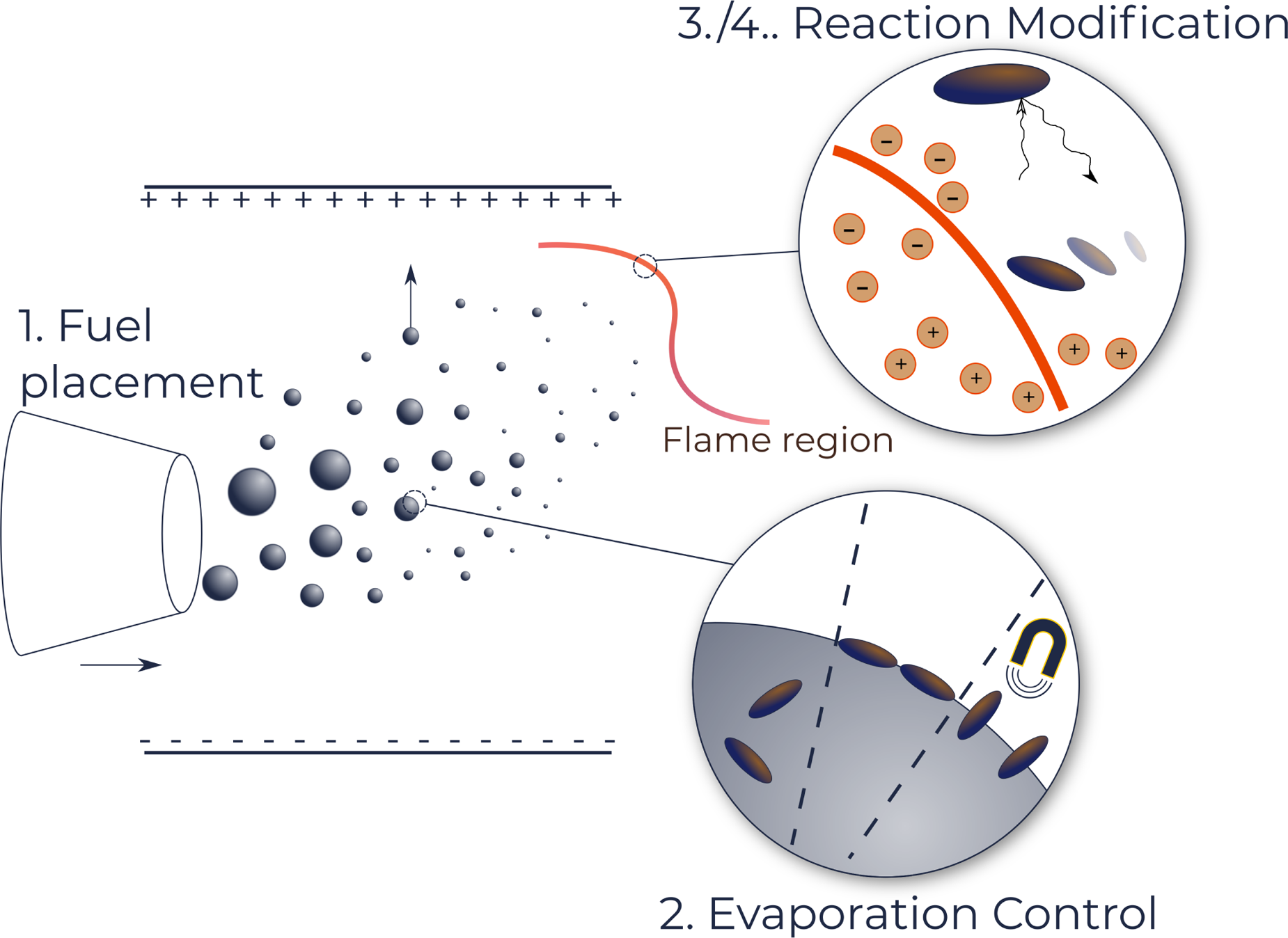

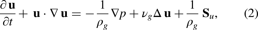
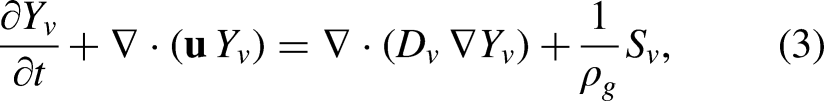
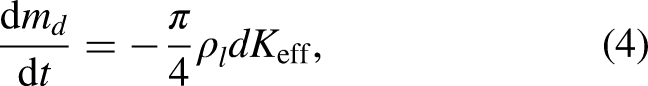
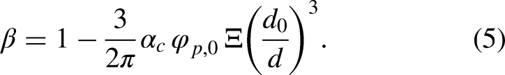
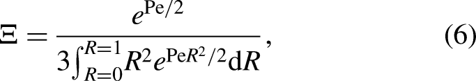
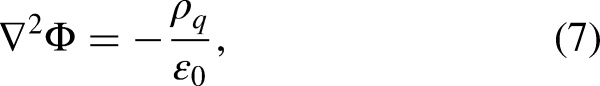

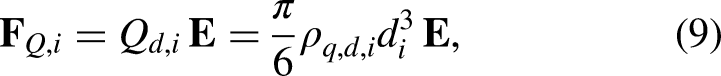
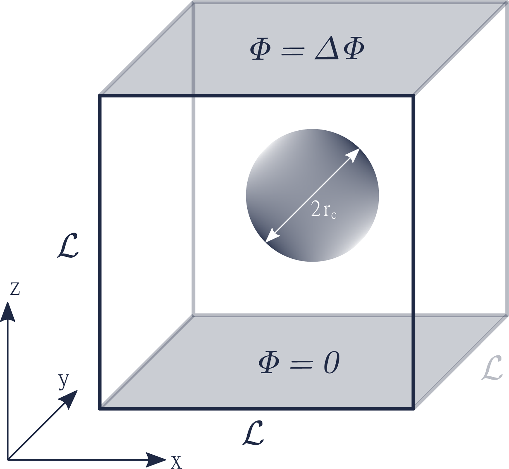
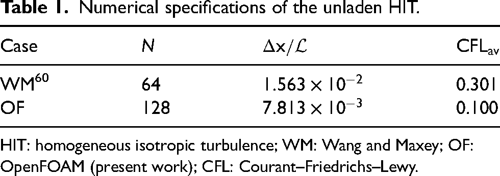
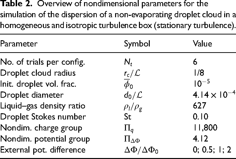
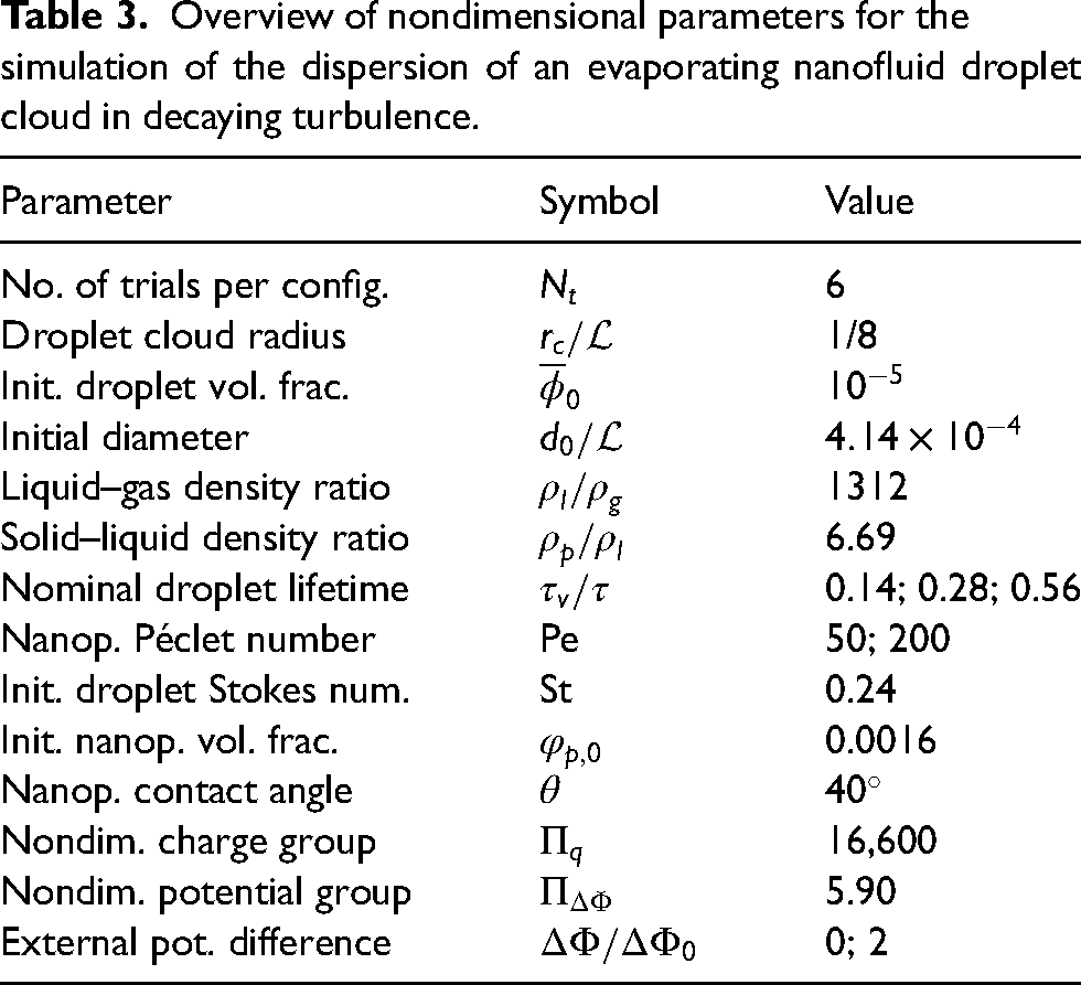
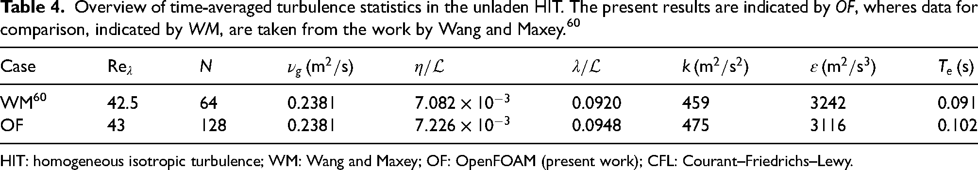

 ) are shown. The red marker represents the initial conditions used in this work for the non-evaporating case in stationary turbulence at
 ). Data points are shown for a volume fraction of
 ).
).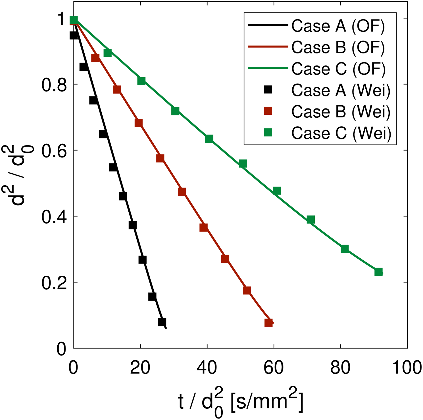
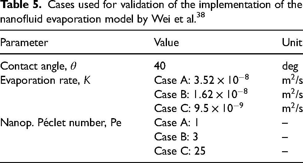

 ),
),  ) and
) and  ).
).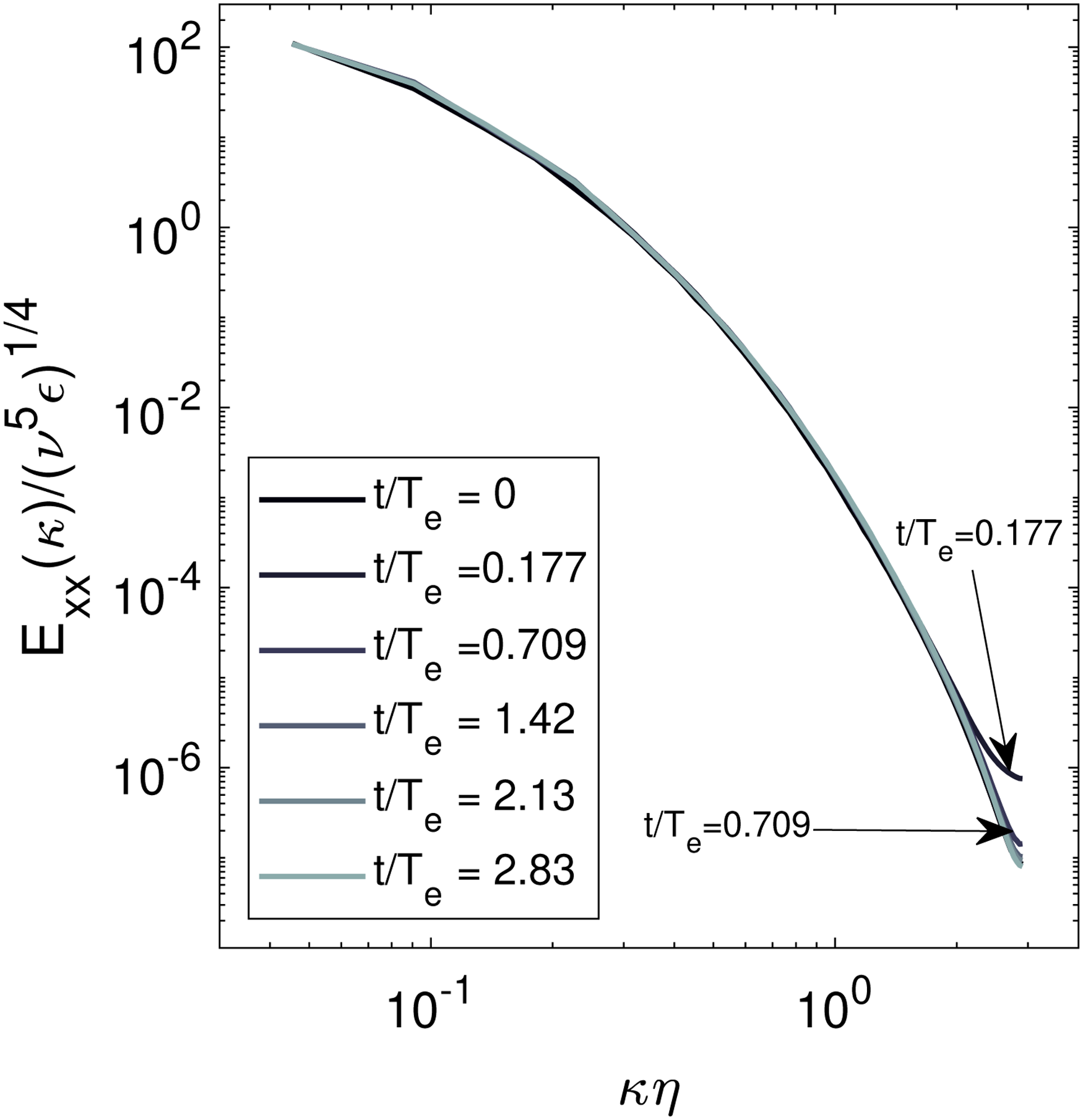
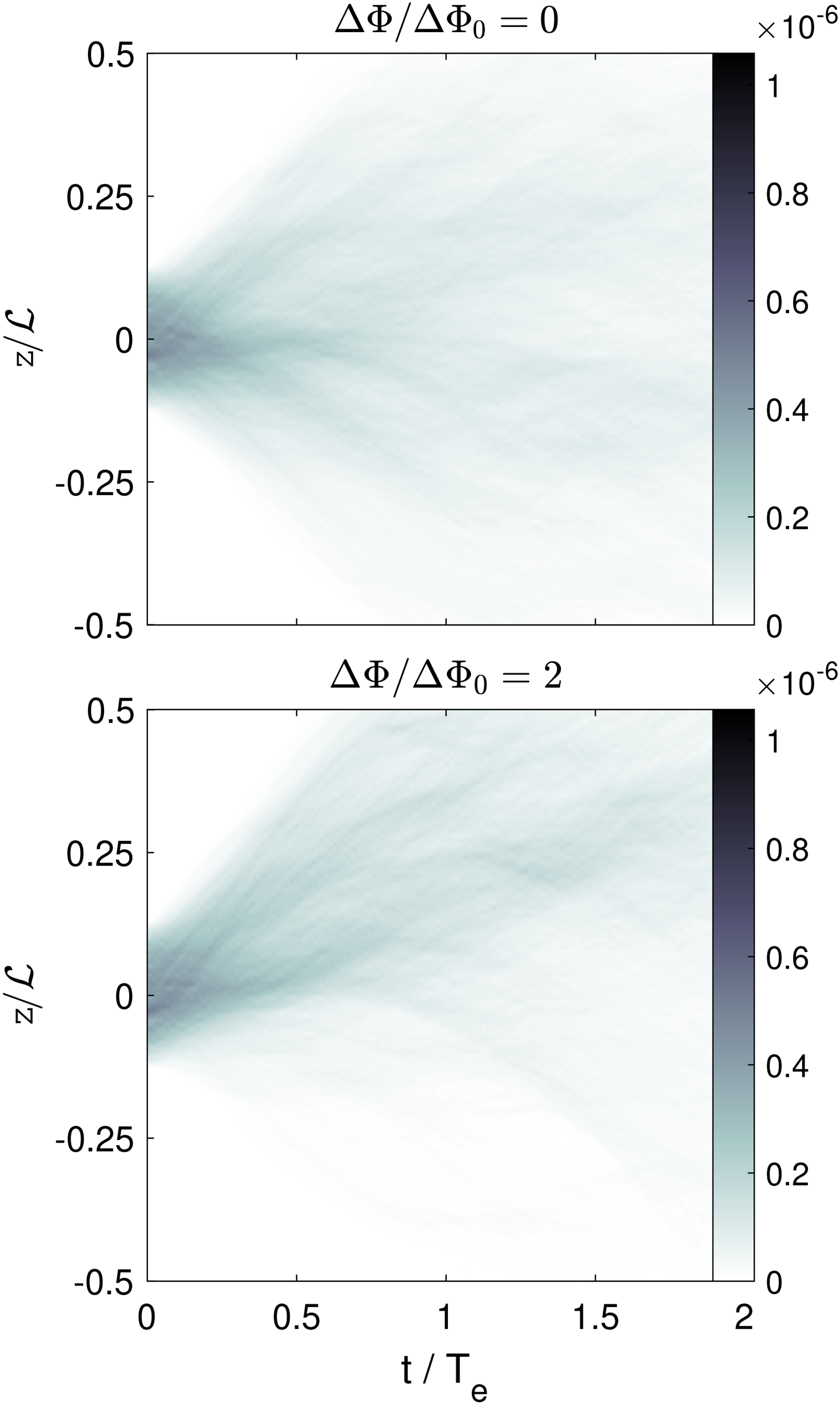

 ),
),  ) and
) and  ). Square markers (
 ) represent the droplet centre of mass and
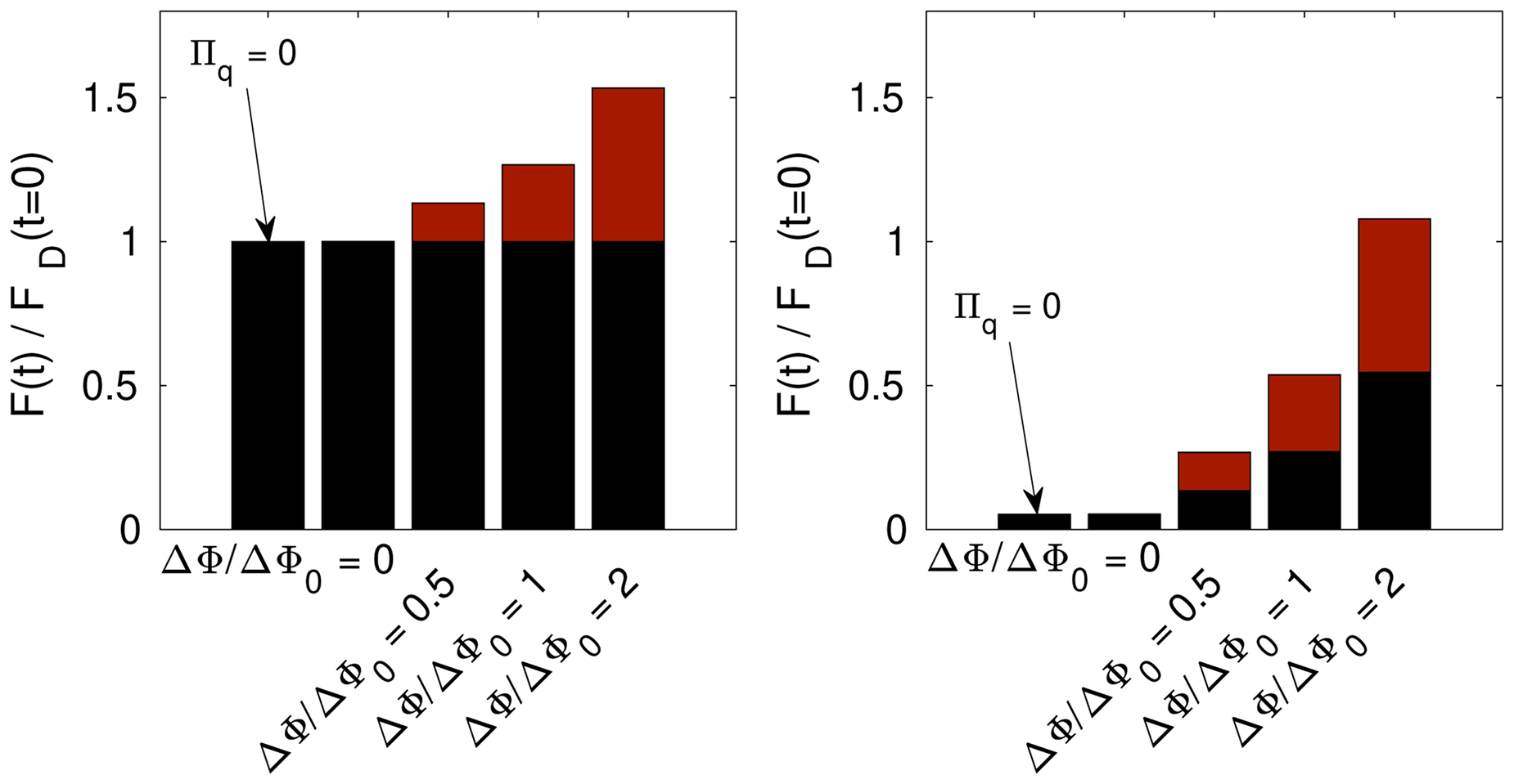

 ),
),  ) and
) and  ).
).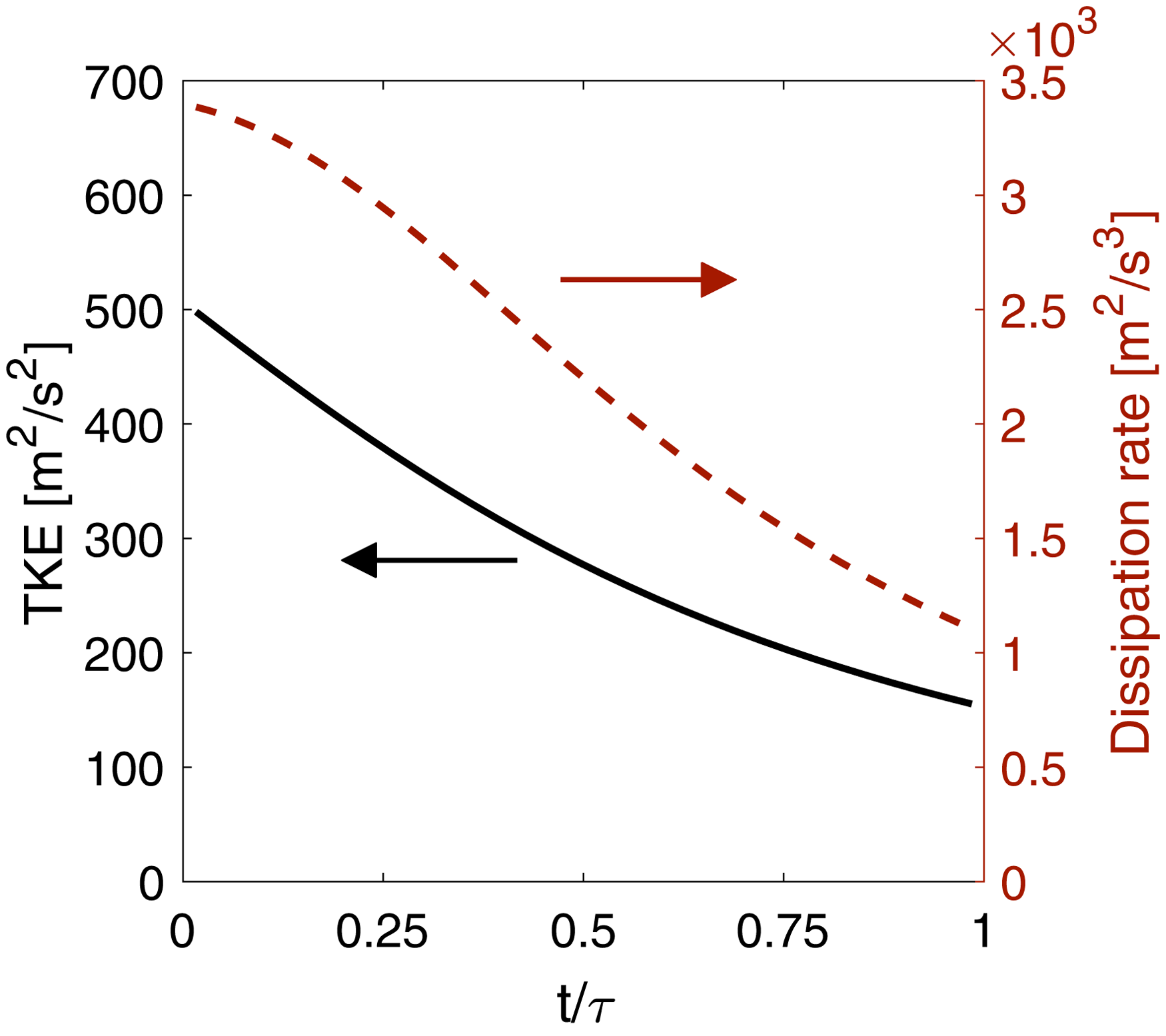

 ),
),  ) and
) and  ) at
) at  ) and
) and  ) in decaying turbulence are shown for reference.
 ) are shown in all plots. Data at different
  ) and
) and  ) in decaying turbulence.
 ) and
) and  ).
).