Assessment of the pseudopotential lattice-Boltzmann method for modeling multiphase fuel droplets

Abstract

An improved pseudopotential lattice–Boltzmann model was proposed for simulating multiphase flow dynamics to describe fuel droplets, and its thermodynamic consistency was tested against the Peng–Robinson equation of state. The studied liquid fuels included paraffinic hydrocarbons with a different number of carbon atoms (C ${}_1$ –C ${}_{10}$ ), methanol (CH ${}_3$ OH), hydrogen (H ${}_2$ ), ammonia (NH ${}_3$ ), and water (H ${}_2$ O). To improve accuracy and reduce the magnitude of the spurious currents, the multi-relaxation times collision operator was implemented and the forcing term was computed using the hybrid pseudopotential interaction force with an eighth-order isotropic degree. The pseudopotential lattice–Boltzmann model accurately predicted the equilibrium densities and captured satisfactorily the thermodynamic vapor-liquid coexistence curve given by the analytical solution of the Peng–Robinson equation of state for acentric factors ranging from $-$ 0.22 to 0.56, keeping the maximum average error for the liquid and vapor branches below 0.8% and 3.7%, respectively. Nevertheless, Peng–Robinson was found to be insufficiently accurate to replicate the actual thermodynamic state, especially for H ${}_2$ O and CH ${}_3$ OH, for which the results strongly deviated from the experimental vapor-liquid equilibrium densities and reached average errors for the vapor phase of nearly 28%. Furthermore, the surface tension ( $\gamma$ ) was retrieved using the multiphase pseudopotential lattice–Boltzmann results and served to verify the thermodynamic consistency of the pseudopotential lattice–Boltzmann with respect to the parachor model. Lastly, the pseudopotential lattice–Boltzmann model was also shown to predict accurately the transient behavior of oscillating droplets. Overall, the enhanced model satisfactorily predicted the properties and behavior of the substances for a wide range of conditions.

Introduction

The understanding of the underlying dynamics and interactions in multiphase flows is of interest to both the scientific and engineering communities due to their relevance in an extensive variety of applications. Different modeling approaches have been proposed to simulate multiphase flows, ranging from macroscopic continuum-based methods (conventional computational fluid dynamics (CFD)) to more fundamental particle dynamics-based discrete methods, such as dissipative particle dynamics, direct simulation Monte–Carlo (MC), and molecular dynamics (MD)^1,2. In between, we find the lattice–Boltzmann (LB) method, which can be interpreted as an Eulerian description of the Boltzmann equation or a numerical method based on kinetic theory to solve conservation equations, allowing to incorporate microscopic dynamics given its mesoscopic nature ^1–4 .

The LB method has not only been successfully applied to simulate hydrodynamic systems, but it has also been attractive in areas of complex fluids such as suspensions, viscoelastic fluids, and multiphase flows^3,4. For the latter, the majority of the proposed LB approaches can be essentially classified into four categories: the color gradient ⁵ , free-energy^6,7, pseudopotential (PP)^8,9, and phase-field^10,11 models. Among these, the pseudopotential lattice–Boltzmann (PP–LB) has gained popularity in multi-phase flow simulations in favor of its conceptual simplicity, easy implementation, capability to capture the non-ideal fluid behavior, robustness for flows at relatively high Reynolds number and high-density ratios, and its ability to capture the interface dynamics such as separation, coalescence, and breakup without the need to employ the interface tracking/capturing technique.

Despite its numerous advantages, a main drawback of the PP–LB method is the possible lack of thermodynamic consistency and large spurious currents around interfaces^12–14, depending on many factors such as the mathematical definition of the interaction potential function^8,15,16, the selection of the collision operator, the interaction force’s isotropy degree ¹² , and the choice of the forcing scheme ¹⁴ .

To overcome the thermodynamic inconsistencies and suppress the spurious velocities at higher density ratios, various strategies have been proposed, including a weighted form of inter-particle interaction force ( ${\mathbf{F}}_{\mathrm{int}}$ ) introduced by Kupershtokh et al. ¹⁵ (also referred to as $\beta$ -scheme and hybrid interaction force ^15–17 ), sophisticated collision operators, modified forcing-schemes that improve the mechanical stability condition ^{13 ,18,19}, and the enforcement of higher isotropic orders^12,18. In an attempt to systematically assess the forcing term of the PP–LB method, Zarghami et al. ¹⁴ evaluated the accuracy, stability, and effect on the spurious currents of different forcing schemes, as well as that of the $\beta$ -scheme^15,17 on the potential term. According to their assessment, exact difference method (EDM) showed the most promising results in terms of accuracy and stability for a wider range of reduced temperature and density ratio. A similar conclusion was obtained by Restrepo et al. ²⁰ , who assessed the effect of the single relaxation time (SRT) and multiple relaxation time (MRT) collision operators along with the multi-range PP on the spurious currents.

Given the lack of comprehensive studies to address the aforementioned issues of thermodynamic consistency for real fluids, Huang et al. ²¹ comprehensively assessed the thermodynamic phase behavior of LB for fluids with curved interfaces, examining the effect of Laplace pressure on the equilibrium densities and saturation pressures of both liquid and vapor phases for methane (CH ${}_4$ ), ethane (C ${}_2$ H ${}_6$ ), nitrogen (N ${}_2$ ), carbon dioxide (CO ${}_2$ ), and water (H ${}_2$ O). They concluded that the equilibrium densities and saturation pressures predicted by LB must not be directly compared with the ones given by Maxwell’s equal area rule owing to the influence of the Laplace pressure on curved interfaces. However, their study is based on the Carnahan–Starling (CS) equation of state (EOS), and as reported by Restrepo Cano et al. ²² , CS EOS is unable to replicate the shape of the vapor-liquid coexistence curves for different types of fluids. In fact, it assumes that the difference among fluids lies exclusively in their critical properties (principle of corresponding states) without considering the effect of non-spherical molecules or presence of polar groups that are correlated with Pitzer’s acentric factor ( ${\omega }_{\mathrm{ac}}$ ).

Recently, Huang et al. ²³ extended the application of PP–LB to study the vapor-liquid equilibrium (VLE) of methane in nanopores under the effects of adsorption using the Peng–Robinson (PR) equation of state (EOS). It was successfully applied to assess the thermodynamic state of CH ${}_4$ and determine the coexistence curve at different sizes of nanochannels. However, this study was limited to just a few components with low acentric factor, such as methane (CH ${}_4$ ). Whether the PP–LB method with PR EOS is able to describe correctly the physical behavior of real fluids for a wide range of increasing acentric factors is yet to be explored.

The present study aims to assess the suitability of PP–LB in describing multiphase fuel droplets by evaluating its thermodynamic consistency and its capability to simulate real fluids with curved interfaces, including a wide range of linear single-bonded hydrocarbons (C ${}_1$ to C ${}_{10}$ ), methanol (CH ${}_3$ OH), hydrogen (H ${}_2$ ), ammonia (NH ${}_3$ ), and water (H ${}_2$ O). Thus, the influence of Pitzer’s acentric factor ( ${\omega }_{\mathrm{ac}}$ ) on both accuracy and stability is also addressed. To reduce the magnitude of the parasitic currents and achieve higher numerical stability without the shortcomings of the standard PP–LB, we implemented the MRT collision operator and the EDM forcing scheme along with the widely used hybrid interaction force ( $\beta$ -scheme) ^{12 , 15–17} and the two-belt discretization for the forcing term (eighth-order of isotropy PP method) ¹² .

Mathematical model

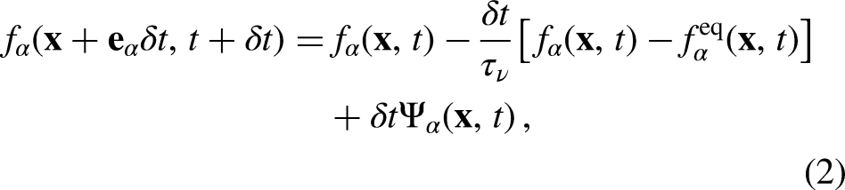
The lattice Boltzmann method describes the time evolution of the density distribution function ( $f_{\alpha }$ ), or populations, for a set of discrete velocities ( ${\mathbf{e}}_{\alpha }$ ), written as

$$f_{\alpha }(\mathbf{x}+{\mathbf{e}}_{\alpha }\delta t,t+\delta t)-f_{\alpha }(\mathbf{x},t)=\delta t{\mathrm{\Omega }}_{\alpha }(\mathbf{x},t)+\delta t{\mathrm{\Psi }}_{\alpha }(\mathbf{x},t),$$

(1)

where f ${}_{\alpha }(\mathbf{x},t)$ and ${\mathrm{\Psi }}_{\alpha }(\mathbf{x},t)$ are the density distribution function and forcing term at position $\mathbf{x}$ and time $t$ , respectively. Using the SRT, also known as Bhatnagar–Gross–Krook (BGK) operator, to describe the collision process, (equation 1) becomes

$$\begin{array}{rl}{f}_{\alpha }(\mathbf{x}+{\mathbf{e}}_{\alpha }\delta t,t+\delta t)=& f_{\alpha }(\mathbf{x},t)-\frac{\delta t}{{\tau }_{\nu }}[f_{\alpha }(\mathbf{x},t)-f_{\alpha }^{\mathrm{eq}}(\mathbf{x},t)]\\ & +\delta t{\mathrm{\Psi }}_{\alpha }(\mathbf{x},t),\end{array}$$

(2)

such that the $f_{\alpha }$ are relaxed linearly towards their local equilibrium density distribution function ( $f_{\alpha }^{\mathrm{eq}}$ ) at a fixed rate determined by the relaxation time ( ${\tau }_{\nu }$ ), which is the characteristic relaxation time obtained from $\nu =c_{\mathrm{s}}^2({\tau }_{\nu }-0.5)\delta t$ , with $\nu$ being the kinematic viscosity of the fluid in the lattice space. Hence, the value of ${\tau }_{\nu }$ must be higher than 0.5 to ensure a positive value of lattice fluid kinematic viscosity ( $\nu$ ) and the numerical stability of the model. The bulk fluid variables in each lattice are constructed from $f_{\alpha }^{\mathrm{eq}}$ by

$$\rho =\sum _{\alpha }{f}_{\alpha }^{\mathrm{eq}}=\sum _{\alpha }{f}_{\alpha },\rho \mathbf{u}=\sum _{\alpha }{\mathbf{e}}_{\alpha }{f}_{\alpha }^{\mathrm{eq}}=\sum _{\alpha }{\mathbf{e}}_{\alpha }{f}_{\alpha },$$

(3)

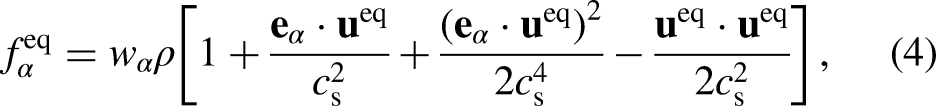
where $\rho$ and $\mathbf{u}$ are the density and velocity, respectively, and $\alpha$ is the index of the direction vector associated with each of the discrete velocities in the lattice. Here $f_{\alpha }^{\mathrm{eq}}$ , obtained via a low-Mach number expansion of the continuum Maxwell–Boltzmann distribution ¹⁴ , has the form

$$f_{\alpha }^{\mathrm{eq}}=w_{\alpha }\rho [1+\frac{{\mathbf{e}}_{\alpha }\cdot {\mathbf{u}}^{\mathrm{eq}}}{c_{\mathrm{s}}^2}+\frac{{({\mathbf{e}}_{\alpha }\cdot {\mathbf{u}}^{\mathrm{eq}})}^2}{2c_{\mathrm{s}}^4}-\frac{{\mathbf{u}}^{\mathrm{eq}}\cdot {\mathbf{u}}^{\mathrm{eq}}}{2c_{\mathrm{s}}^2}],$$

(4)

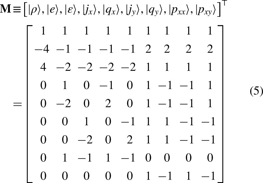
where $w_{\alpha }$ is a weighting factor. For a two-dimensional case, one common velocity discretization is the 2-dimensions, 9-velocity lattice scheme (D ${}_2$ Q ${}_9$ ). For D ${}_2$ Q ${}_9$ and unit lattice speed ( $c={\delta }_x/{\delta }_t=1$ and ${\delta }_x={\delta }_t=1$ ), the ${\mathbf{e}}_{\alpha }$ in the $\alpha$ -direction is explicitly given as follows:

$${\mathbf{e}}_{\alpha }=\{\begin{array}{cc}(0,0{)}^{\mathrm{\top }},& \alpha =0,\\ {(\cos [(\alpha -1)\pi /2],\sin [(\alpha -1)\pi /2])}^{\mathrm{\top }},& \alpha =[1,4],\\ \sqrt{2}{(\cos [(2\alpha -1)\pi /4],\sin [(2\alpha -1)\pi /4])}^{\mathrm{\top }},& \alpha =[5,8],\end{array}$$

where ${\mathbf{e}}_{1-4}$ and ${\mathbf{e}}_{5-8}$ represent the rectangular and diagonal discrete velocities, respectively. For the D ${}_2$ Q ${}_9$ , the weights ( $w_{\alpha }$ ) are given by $w_0=4/9$ , $w_{1-4}=1/9$ , and $w_{5-8}=1/36$ .

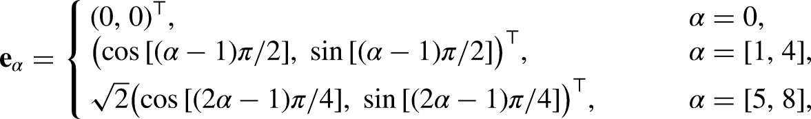
The above relaxation assumes a SRT. While such a collision operator is simple and computationally efficient, it may lead to numerical instability by enforcing the entire set of populations ³ ( $f_{\alpha }$ ) to relax at a single characteristic time. One way to overcome this shortcoming is by implementing a moment-based collision operator to allow MRTs, wherein the populations are first mapped onto the moment space and then relaxed independently at their own rate. Therefore, the implementation of MRT allows an independent control of individual relaxation modes ³ . To perform the collision step, the population functions are first mapped onto the moment space by a transformation matrix ( $\mathbf{M}$ ), written as

$$|m_{\alpha }⟩=\mathbf{M}|f_{\alpha }⟩,|f_{\alpha }⟩={\mathbf{M}}^{-1}|m_{\alpha }⟩,$$

where $|\cdot ⟩$ denotes a column vector. In this work, the Gram–Schmidt transformation matrix $\mathbf{M}$ is used, in which the row vectors are organized in terms of the corresponding tensor. The first three rows correspond to scalars or zeroth-order tensors $\rho$ , $e$ , $\epsilon$ , which represent the density mode, energy mode, and energy square, respectively. The following four rows correspond to first-order tensors $j_x$ , $q_x$ , $j_y$ , and $q_y$ , which denote the $x$ and $y$ components of the momentum ( $\mathit{j}$ ) and energy flux ( $\mathit{q}$ ) vectors. Finally, the last two rows correspond to the diagonal and off-diagonal of the pressure tensor (second-order tensor). Thus, the transformation matrix $\mathbf{M}$ can be explicitly written as^3,24

$$\begin{array}{rl}\mathbf{M}& \equiv {[|\rho ⟩,|e⟩,|\epsilon ⟩,|j_x⟩,|q_x⟩,|j_y⟩,|q_y⟩,|p_{xx}⟩,|p_{xy}⟩]}^{\mathrm{\top }}\\ & =\left[\begin{array}{ccccccccc}1& 1& 1& 1& 1& 1& 1& 1& 1\\ -4& -1& -1& -1& -1& 2& 2& 2& 2\\ 4& -2& -2& -2& -2& 1& 1& 1& 1\\ 0& 1& 0& -1& 0& 1& -1& -1& 1\\ 0& -2& 0& 2& 0& 1& -1& -1& 1\\ 0& 0& 1& 0& -1& 1& 1& -1& -1\\ 0& 0& -2& 0& 2& 1& 1& -1& -1\\ 0& 1& -1& 1& -1& 0& 0& 0& 0\\ 0& 0& 0& 0& 0& 1& -1& 1& -1\end{array}\right]\end{array}$$

(5)

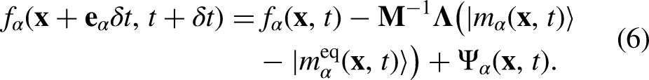
Consequently, different moments are relaxed at their own collision rates, comprised in the relaxation matrix ( $\mathbf{\Lambda }$ ), which are given by $\mathbf{\Lambda }\equiv \mathrm{diag}({\tau }_{\rho }^{-1},{\tau }_e^{-1},{\tau }_{\zeta }^{-1},{\tau }_j^{-1},{\tau }_q^{-1},{\tau }_j^{-1},{\tau }_q^{-1},{\tau }_{\nu }^{-1},{\tau }_{\nu }^{-1})$ . Note that MRT reduces to SRT when the inverse of the relaxation times in $\mathbf{\Lambda }$ are replaced by ${\tau }_{\nu }^{-1}$ . Finally, the post-collision moments are mapped back onto the population space using the inverse of $\mathbf{M}$ and the propagation step is carried out. The LB equation (equation 1), incorporating the MRT collision operator, takes the form

$$\begin{array}{rl}{f}_{\alpha }(\mathbf{x}+{\mathbf{e}}_{\alpha }\delta t,t+\delta t)=& f_{\alpha }(\mathbf{x},t)-{\mathbf{M}}^{-1}\mathbf{\Lambda }(|m_{\alpha }(\mathbf{x},t)⟩\\ & -|m_{\alpha }^{\mathrm{eq}}(\mathbf{x},t)⟩)+{\mathrm{\Psi }}_{\alpha }(\mathbf{x},t).\end{array}$$

(6)

Note that the previous equation is written exclusively for a $\mathbf{\Lambda }$ -independent forcing term ( ${\mathrm{\Psi }}_{\alpha }$ ), such as the EDM ¹⁵ forcing scheme, which is implemented in this work due to its simplicity and numerical stability. By implementing the EDM scheme, ${\mathrm{\Psi }}_{\alpha }$ is simply computed as the difference of the $f_{\alpha }^{\mathrm{eq}}$ before and after the action of the external net force ( $\mathbf{F}$ )

$${\mathrm{\Psi }}_{\alpha }=f_{\alpha }^{\mathrm{eq}}(\rho ,\mathbf{u}+\frac{\mathbf{F}\delta t}{\rho })-f_{\alpha }^{\mathrm{eq}}(\rho ,\mathbf{u}).$$

(7)

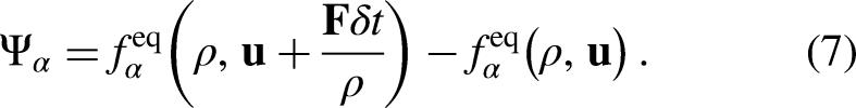
Given that the EDM scheme is $\mathbf{\Lambda }$ -independent, for any moment-based collision operator (e.g., MRT and the central moment, also known as the cascaded operator) the collision can be carried out in the moment space as a force-free process (i.e., taking ${\mathrm{\Psi }}_{\alpha }=0$ , and simply adding the ${\mathrm{\Psi }}_{\alpha }$ term in the population space prior to the streaming step). In equation 7, the external net force, $\mathbf{F}$ , is expressed as the sum of any external force acting on a fluid particle, e.g., fluid-fluid ( ${\mathbf{F}}_{\mathrm{f}-\mathrm{f}}$ ) and solid-fluid interaction force, gravitational force, electrical force, etc. Due to the action of $\mathbf{F}$ , the local equilibrium velocity ( ${\mathbf{u}}^{\mathrm{eq}}$ ) and actual fluid velocity ( $\mathbf{U}$ ) are calculated as the average of those associated with the momentum before and after the collision step ¹⁵

$$\mathbf{U}={\mathbf{u}}^{\mathrm{eq}}=\mathbf{u}+\frac{\delta t}{2\rho }\mathbf{F}.$$

(8)

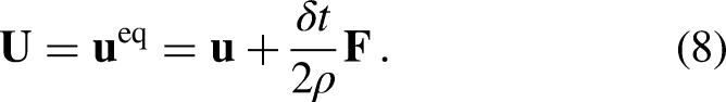
The macroscopic Navier–Stokes (NS) equations obtained by the Chapman–Enskog expansion of the PP–LB model using the EDM scheme include an extra non-linear term, containing the term ${\tau }_{\nu }\mathrm{\nabla }\cdot ({\rho }^{-1}\mathbf{F}\mathbf{F})$ , which has been shown to enhance the stability of the scheme^13,14,25,26. However, due to the extra terms added by EDM to the macroscopic NS equations, the predicted equilibrium densities are influenced by the value of ${\tau }_{\nu }$ ^13,14. Such a dependency may be suppressed by implementing a moment-based collision operator with a correct relaxation matrix instead of SRT. For a single-component multiphase system, in which the fluid-fluid interaction is the only force acting on the fluid particles, $\mathbf{F}$ = ${\mathbf{F}}_{\mathrm{f}-\mathrm{f}}$ and is expressed as follows^8,9:

$${\mathbf{F}}_{\mathrm{f}-\mathrm{f}}(\mathbf{x},t)=-\psi (\mathbf{x},t)\mathcal{G}\sum _{\alpha }{w}_{\alpha }\psi (\mathbf{x}+{\mathbf{e}}_{\alpha },t){\mathbf{e}}_{\alpha },$$

(9)

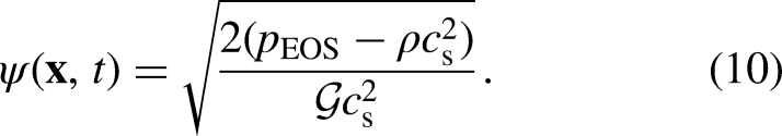
where $\mathcal{G}$ is a parameter that controls the interaction strength, being negative for attractive interactions and positive for repulsive ones. The local-density PP function ( $\psi$ ), which describes the fluid-fluid interactions that are triggered by density inhomogeneities, is written in the following form to incorporate the EOS into the PP–LB ²⁷ :

$$\psi (\mathbf{x},t)=\sqrt{\frac{2(p_{\mathrm{EOS}}-\rho c_{\mathrm{s}}^2)}{\mathcal{G}{c}_{\mathrm{s}}^2}}.$$

(10)

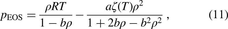
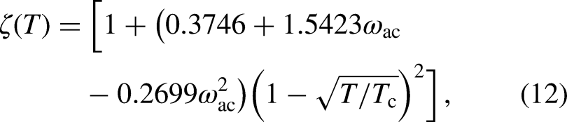
In this study, $p_{\mathrm{EOS}}$ was calculated using the PR EOS, given by

$$p_{\mathrm{EOS}}=\frac{\rho RT}{1-b\rho }-\frac{a\zeta (T){\rho }^2}{1+2b\rho -b^2{\rho }^2},$$

(11)

$$\begin{array}{rl}\zeta (T)=& [1+(0.3746+1.5423{\omega }_{\mathrm{ac}}\\ & -0.2699{\omega }_{\mathrm{ac}}^2){(1-\sqrt{T/T_{\mathrm{c}}})}^2],\end{array}$$

(12)

where $a\approx 0.45724R^2{T}_{\mathrm{c}}^2/p_{\mathrm{c}}$ and $b\approx 0.0778R{T}_{\mathrm{c}}/p_{\mathrm{c}}$ . For the simulations, the constants $a$ , $b$ , and $R$ were set to 2/49, 2/21, and 1, respectively ²⁷ . Thus, for the given $a$ , $b$ , and $R$ , the critical temperature ( $T_{\mathrm{c}}$ ), critical pressure ( $p_{\mathrm{c}}$ ), and critical density ( ${\rho }_{\mathrm{c}}$ ) are equal to 0.07292, 0.05956, and 2.6573, respectively, in LB units. To represent different kinds of fluids using the PR EOS, the parameter ${\omega }_{\mathrm{ac}}$ was varied from $-$ 0.22 to 0.56.

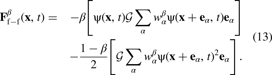
To improve the accuracy of equation 9, the hybrid interaction force, called $\beta$ -scheme^{14,15, 17} , was implemented, where the weighting factor ( $\beta$ ) can be tuned to achieve an optimum order of isotropy:

$$\begin{array}{cc}{\mathbf{F}}_{\mathrm{f}-\mathrm{f}}^{\beta }(\mathbf{x},t)=& -\beta [\psi (\mathbf{x},t)\mathcal{G}{\displaystyle \sum _{\alpha }{w}_{\alpha }^{\beta }\psi (\mathbf{x}+{\mathbf{e}}_{\alpha },t){\mathbf{e}}_{\alpha }}]\\ & -\frac{1-\beta }{2}\left[\mathcal{G}{\displaystyle \sum _{\alpha }{w}_{\alpha }^{\beta }\psi (\mathbf{x}+{\mathbf{e}}_{\alpha },t{)}^2{\mathbf{e}}_{\alpha }}\right].\end{array}$$

(13)

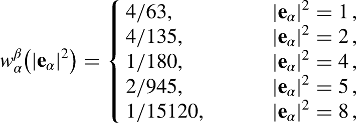
In addition, to reach a higher density ratio ( ${\rho }^{*}$ ) and reduce the magnitude of the spurious velocity ( ${\mathrm{U}}^{\mathrm{s}}$ )^12,20, we enforced an eighth-order isotropic degree in the $\beta$ -scheme (equation 13) by considering the influence of more lattices (D ${}_2$ Q ${}_{25}$ ), and thus controlling the diffusive interface thickness without altering the magnitude of the pressure tensor ¹⁹ by changing the value of $a$ and modifying the contribution of the non-idealities in the PR EOS (equation 11). The weights ( $w_{\alpha }^{\beta }$ ) in equation 13 were set as follows:

$$w_{\alpha }^{\beta }(|{\mathbf{e}}_{\alpha }{|}^2)=\{\begin{array}{cc}4/63,& |{\mathbf{e}}_{\alpha }{|}^2=1,\\ 4/135,& |{\mathbf{e}}_{\alpha }{|}^2=2,\\ 1/180,& |{\mathbf{e}}_{\alpha }{|}^2=4,\\ 2/945,& |{\mathbf{e}}_{\alpha }{|}^2=5,\\ 1/15120,& |{\mathbf{e}}_{\alpha }{|}^2=8,\end{array}$$

where $|{\mathbf{e}}_{\alpha }{|}^2$ is computed as $|{\mathbf{e}}_{\alpha }{|}^2=e_{\alpha ,x}^2+e_{\alpha ,y}^2$ . As mentioned above, in a recent study Restrepo Cano et al. ²⁰ noted that the implementation of Kupershtokh’s EDM, enforcing a multirange hybrid interaction force, can enhance both the accuracy and numerical stability of the PP–LB method, which favors the reduction of the magnitude of the spurious currents for systems considering fluids with curved interfaces. Thus, the selection of this model is suitable for the following thermodynamic consistency study on droplets.

Results and discussion

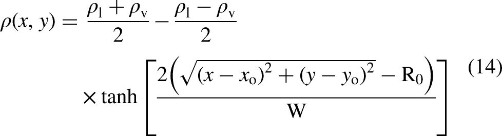
An in-house C++ solver was developed for PP–LB simulations and parallelized with the message passing interface library, implementing the above-mentioned schemes. Simulations of a stationary suspended droplet were carried out to determine both the equilibrium density of the liquid ( ${\rho }_{\mathrm{l}}$ ) and the vapor ( ${\rho }_{\mathrm{v}}$ ) phase. Subsequently, the pressure difference was determined to retrieve the surface tension using the Laplace–Young equation. The initial condition was set by locating a liquid droplet in the center $(x_{\mathrm{o}},y_{\mathrm{o}})$ of a 200 by 200 fully periodic zero-velocity computational domain. The initial density field was described by a hyperbolic tangent function (see equation 14), where the liquid and vapor density were given by the EOS at a specified temperature.

$$\begin{array}{rl}\rho (x,y)=& \frac{{\rho }_{\mathrm{l}}+{\rho }_{\mathrm{v}}}{2}-\frac{{\rho }_{\mathrm{l}}-{\rho }_{\mathrm{v}}}{2}\\ & \times \tanh \left[\frac{2(\sqrt{(x-x_{\mathrm{o}}{)}^2+(y-y_{\mathrm{o}}{)}^2}-{\mathrm{R}}_0)}{\mathrm{W}}\right]\end{array}$$

(14)

The prescribed interface width ( $\mathrm{W}$ ) and initial droplet radius ( ${\mathrm{R}}_0$ ) were set to 5 and 30 lattice nodes, respectively. Note that, for the Laplace–Young numerical tests, the radius was varied from 25 to 40 lattices. The relaxation times for the 9 moments in $\mathbf{\Lambda }$ of equation 6 are given by ${\tau }_{\rho }^{-1}={\tau }_j^{-1}=$ 1 and ${\tau }_e^{-1}={\tau }_{\zeta }^{-1}={\tau }_q^{-1}=$ 1.1, while ${\tau }_{\nu }^{-1}$ is determined according to the value of $\nu$ .

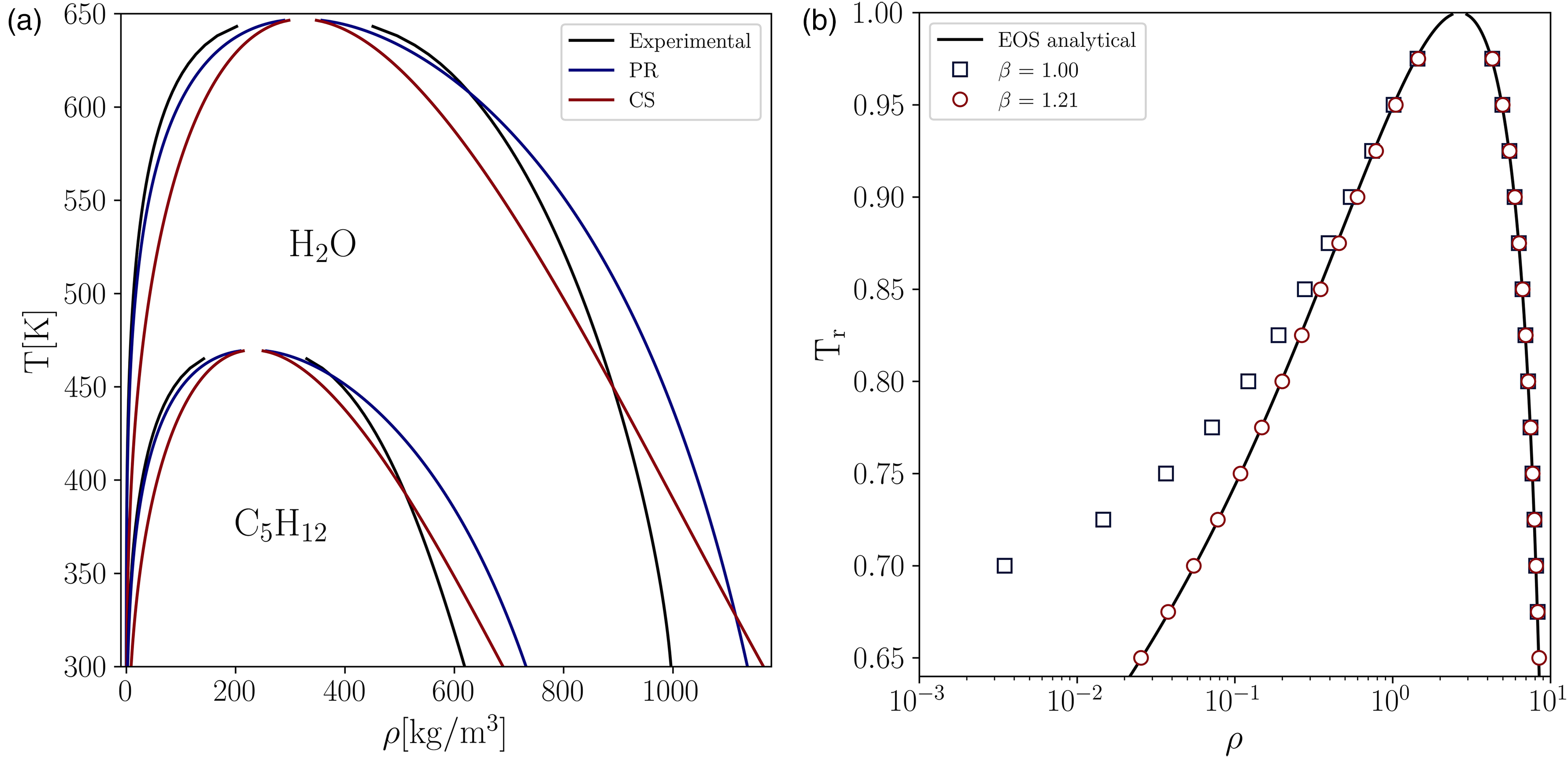
First, to illustrate the superiority of the PR EOS over the CS EOS in representing the thermodynamic state of real substances, we compared the analytical solution of both EOS, given by Maxwell’s equal area rule, to the experimental coexistence curve for two representative substances, namely water (H ${}_2$ O) and n-pentane (C ${}_5$ H ${}_{12}$ ). For the CS EOS, we set the parameters $a$ , $b$ , and $R$ equal to 1, 4, and 1, respectively, similar to previous studies ^{14 , 22 , 27} .

As shown in Figure 1(a), we found that the PR EOS is able to capture qualitatively the shape of the experimental vapor-liquid equilibrium VLE curve, whereas the CS EOS does not reproduce the behavior of the liquid branch, exhibiting a more linear-like trend. Hence, CS EOS fails to qualitatively reproduce the coexistence curve of both H ${}_2$ O and C ${}_5$ H ${}_{12}$ . Based on this initial result, for the LB simulations only the PR EOS is adopted. Additionally, to illustrate the influence of the parameter $\beta$ of the hybrid interaction force (equation 13) on accuracy, the coexistence curve for water ( ${\omega }_{\mathrm{ac}}$ = 0.344) obtained with two different $\beta$ (before and after tuning), is displayed in Figure 1(b). Note that when $\beta =1$ , equation 13 reduces to the original interaction force equation 9. The deviation of the original interaction force ( $\beta =1$ ) is evident in Figure 1(b), showing that it suffers to accurately predict the equilibrium vapor density for density ratios greater than 10, i.e., at reduced temperatures below 0.9, reaching deviations for density of the vapor phase ( ${\rho }_{\mathrm{v}}$ ) higher than one order of magnitude at low reduced temperatures. The accuracy of the PP–LB can be remarkably improved by simply setting $\beta =1.21$ , keeping the average error for the predicted liquid and vapor densities below 2%.

Figure 1.

(a) Comparison between the experimental data and the analytical vapor-liquid coexistence curve given by the PR EOS and CS EOS for two representative substances. (b) Effect of $\beta$ on the accuracy of the PP–LB compared to the analytical solution given by Maxwell’s equal area rule and using PR EOS for water ( ${\omega }_{\mathrm{ac}}$ = 0.344). PR EOS: Peng–Robinson equation of state; CS: Carnahan–Starling; PP–LB: pseudopotential lattice–Boltzmann.

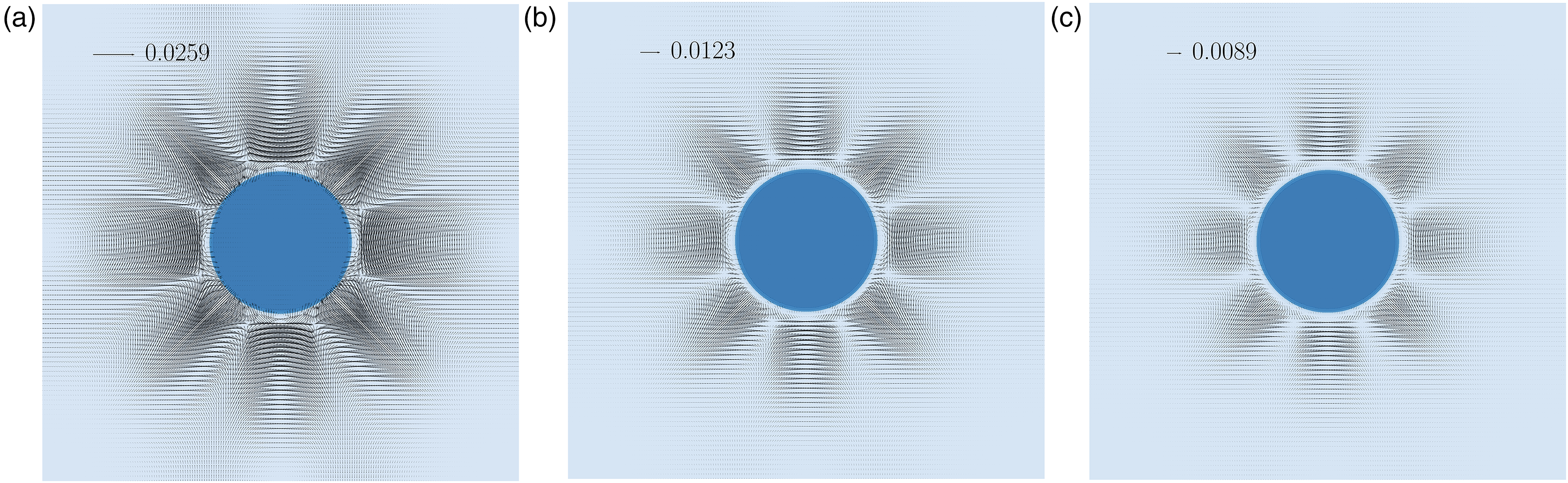
To demonstrate the effect of the collision operator and isotropic order on the magnitude of the spurious currents ( ${\mathrm{U}}^{\mathrm{s}}$ ), an equilibrated stationary circular water droplet ( ${\omega }_{\mathrm{ac}}$ = 0.344) in a gravity-free environment at T ${}_{\mathrm{r}}$ = 0.7 was simulated using different combinations of collision operator and the pseudo-potential tensor order (see Figure 2). A remarkable reduction on ${\mathrm{U}}^{\mathrm{s}}$ is achieved by implementing the proposed MRT collision operator with an eighth-order isotropic interaction force (Figure 2(c)), reducing the ${\mathrm{U}}^{\mathrm{s}}$ by a factor close to 3 compared to the standard SRT with the conventional fourth-order interaction force (Figure 2(a)).

Figure 2.

Spurious velocities distribution over a water liquid droplet on vapor at a reduced temperature of 0.7 for different collision operators and orders of isotropy of the interaction force.

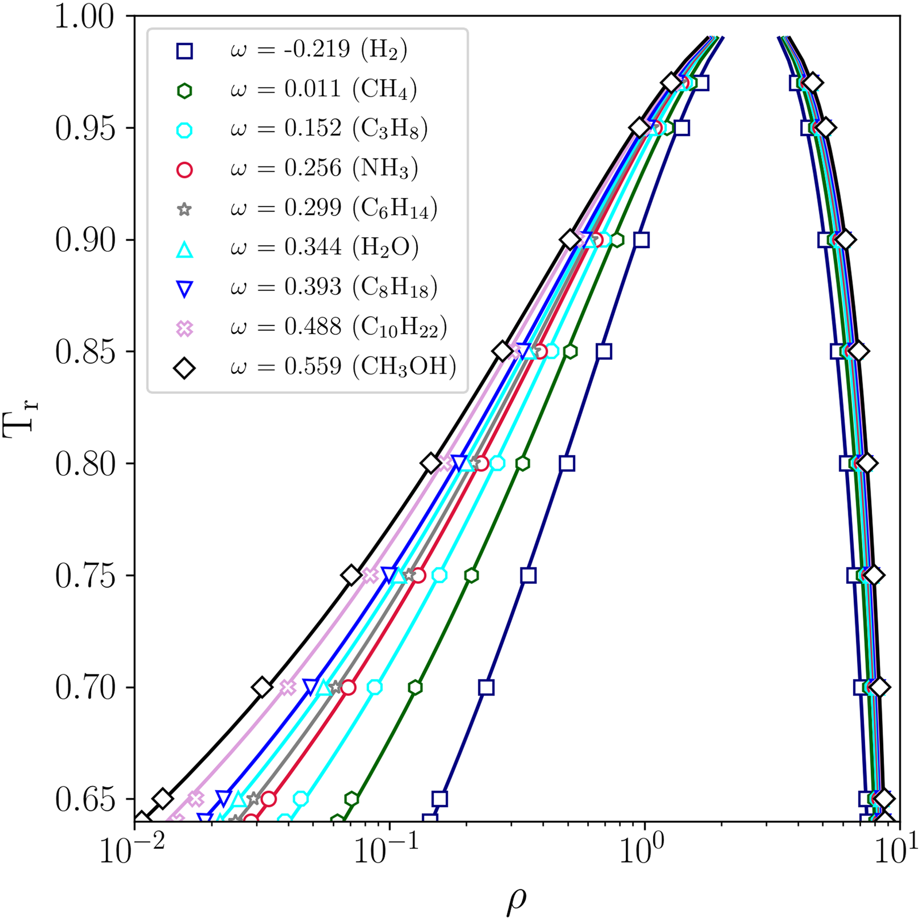
After demonstrating the higher fidelity provided by the selected schemes for PP-LB along with the PR EOS, a comparison was made between the equilibrium densities that are given by the analytical solution of PR EOS and those predicted by the PP–LB simulations for all the substances under consideration. Figure 3 shows the analytical VLE coexistence curve for different values of ${\omega }_{\mathrm{ac}}$ , corresponding to the substances of interest of this work, and the VLE densities predicted by the PP–LB method, utilizing the MRT collision operator and an eighth-order isotropic interaction force, while fixing the weighting factor $\beta$ to 1.21 in equation 13.

Figure 3.

Comparison between the analytical vapor-liquid coexistence curve given by PR EOS and the densities predicted by LB method for different acentric factors ( ${\omega }_{\mathrm{ac}}$ ), implementing an eighth-order isotropic tensor. Analytical solution obtained using Maxwell’s equal area rule (solid lines); LB–MRT results (markers). MRT: multiple relaxation time; LB: lattice–Boltzmann; PR EOS: Peng–Robinson equation of state.

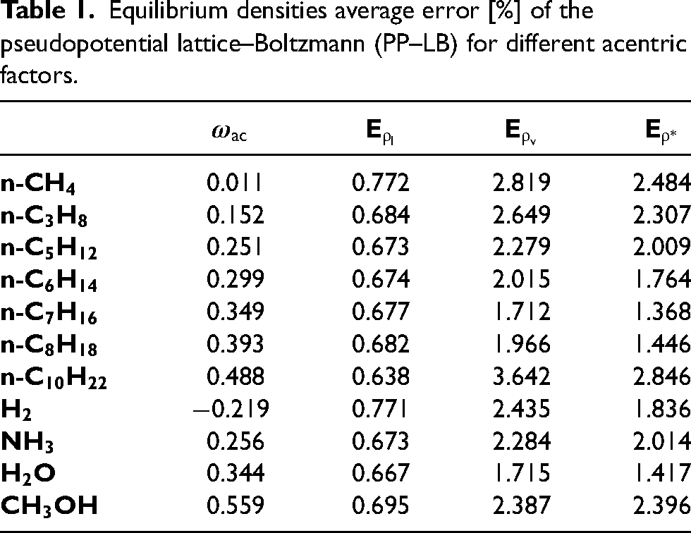
A good agreement is seen between the predictions by the PP–LB and the analytical solution. Additionally, the effect of Pitzer’s acentric factor ( ${\omega }_{\mathrm{ac}}$ ) can be observed in Figure 3, showing that as the value of ${\omega }_{\mathrm{ac}}$ increases, the VLE coexistence curve becomes wider. The average error for the liquid and vapor branches as well as that of the density ratio ( ${\rho }^{*}$ ), for different values of ${\omega }_{\mathrm{ac}}$ , are summarized in Table 1.

Table 1.

Equilibrium densities average error [%] of the pseudopotential lattice–Boltzmann (PP–LB) for different acentric factors.

	${\mathit{\omega }}_{\mathrm{ac}}$	${\mathbf{E}}_{{\rho }_{\mathrm{l}}}$	${\mathbf{E}}_{{\rho }_{\mathrm{v}}}$	${\mathbf{E}}_{{\rho }^{*}}$
n- $\mathbf{C}{\mathbf{H}}_{\mathbf{4}}$	0.011	0.772	2.819	2.484
n- ${\mathbf{C}}_{\mathbf{3}}{\mathbf{H}}_{\mathbf{8}}$	0.152	0.684	2.649	2.307
n- ${\mathbf{C}}_{\mathbf{5}}{\mathbf{H}}_{\mathbf{12}}$	0.251	0.673	2.279	2.009
n- ${\mathbf{C}}_{\mathbf{6}}{\mathbf{H}}_{\mathbf{14}}$	0.299	0.674	2.015	1.764
n- ${\mathbf{C}}_{\mathbf{7}}{\mathbf{H}}_{\mathbf{16}}$	0.349	0.677	1.712	1.368
n- ${\mathbf{C}}_{\mathbf{8}}{\mathbf{H}}_{\mathbf{18}}$	0.393	0.682	1.966	1.446
n- ${\mathbf{C}}_{\mathbf{10}}{\mathbf{H}}_{\mathbf{22}}$	0.488	0.638	3.642	2.846
${\mathbf{H}}_{\mathbf{2}}$	$-$ 0.219	0.771	2.435	1.836
$\mathbf{N}{\mathbf{H}}_{\mathbf{3}}$	0.256	0.673	2.284	2.014
${\mathbf{H}}_{\mathbf{2}}\mathbf{O}$	0.344	0.667	1.715	1.417
$\mathbf{C}{\mathbf{H}}_{\mathbf{3}}\mathbf{O}\mathbf{H}$	0.559	0.695	2.387	2.396

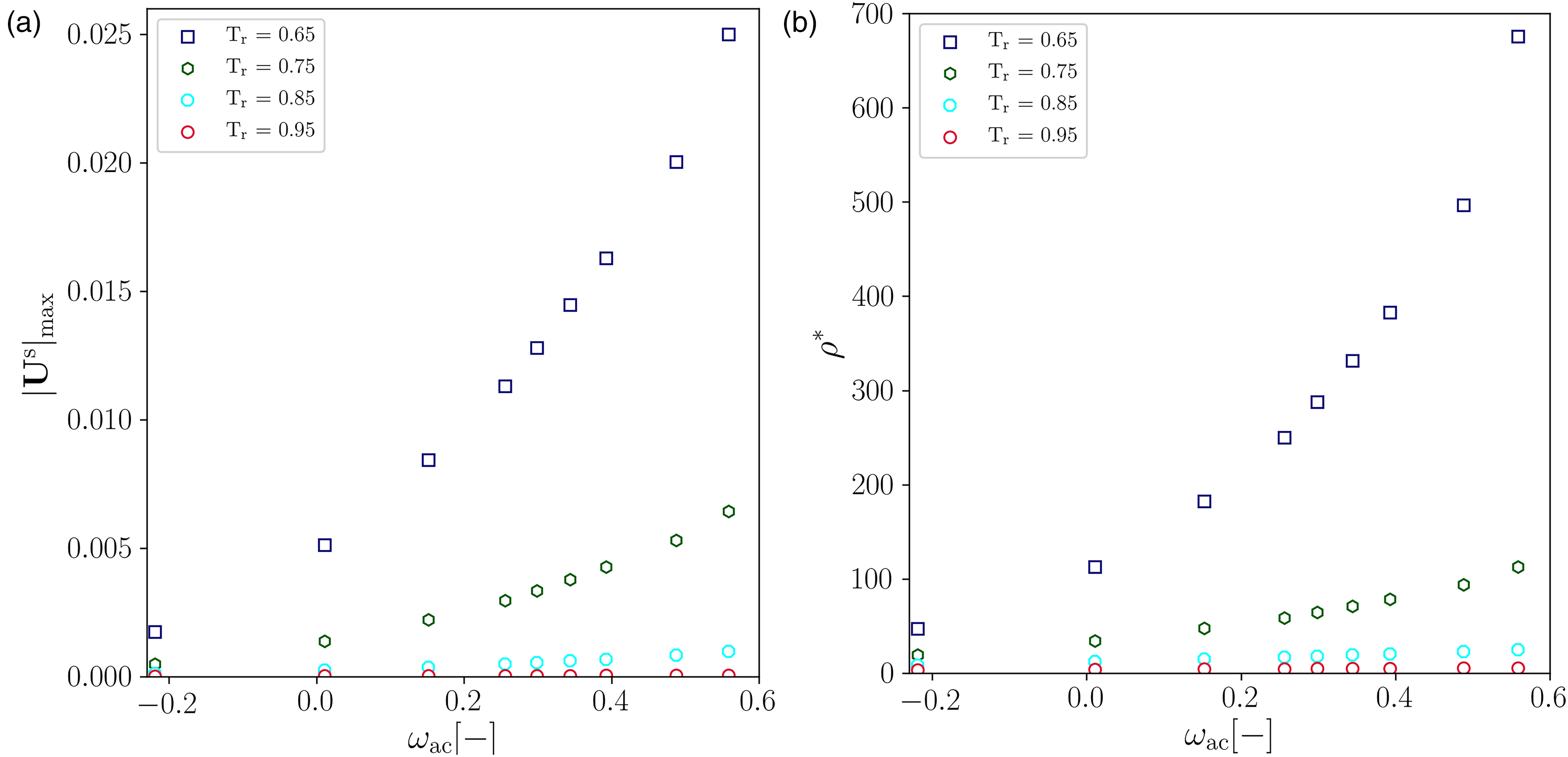
Although the largest average error corresponds to the vapor branch, it did not exceed 3% for all substances except for n-decane ( ${\omega }_{\mathrm{ac}}=0.488$ ). Concerning the effect of ${\omega }_{\mathrm{ac}}$ on the magnitude of the ${\mathrm{U}}^{\mathrm{s}}$ and ${\rho }^{*}$ , Figure 4(a) showed that the magnitude of ${\mathrm{U}}^{\mathrm{s}}$ increases as ${\omega }_{\mathrm{ac}}$ increases. This is due to the direct relation between ${\omega }_{\mathrm{ac}}$ and the shape of the liquid-vapor coexistence curve, in which ${\rho }^{*}$ grows as ${\omega }_{\mathrm{ac}}$ increases. Consequently, the minimum temperature achievable by PP–LB is limited at high values of ${\omega }_{\mathrm{ac}}$ , i.e., the range of temperature for which the PP–LB is stable noticeably reduces at high ${\omega }_{\mathrm{ac}}$ .

Figure 4.

Effect of the acentric factor on the spurious currents and the density ratio at different reduced temperatures. (a) Variation of $|\mathrm{U}{|}_{\max }^{\mathrm{s}}$ . (b) Variation of ${\rho }^{*}$ .

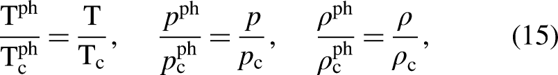
Subsequently, the LB equilibrium density results for different linear single-bonded hydrocarbons (C ${}_1$ –C ${}_{10}$ ), methanol (CH ${}_3$ OH), hydrogen (H ${}_2$ ), ammonia (NH ${}_3$ ), and water (H ${}_2$ O) were converted from lattice units to physical ones to make a direct comparison with the experimental data of the NIST databank ²⁸ . The unit conversion for temperature, pressure, and density was carried out using the principle of corresponding states.

$$\frac{{\mathrm{T}}^{\mathrm{ph}}}{{\mathrm{T}}_{\mathrm{c}}^{\mathrm{ph}}}=\frac{\mathrm{T}}{{\mathrm{T}}_{\mathrm{c}}},\frac{p^{\mathrm{ph}}}{p_{\mathrm{c}}^{\mathrm{ph}}}=\frac{p}{p_{\mathrm{c}}},\frac{{\rho }^{\mathrm{ph}}}{{\rho }_{\mathrm{c}}^{\mathrm{ph}}}=\frac{\rho }{{\rho }_{\mathrm{c}}},$$

(15)

In the equations above, the superscript “ph” and subscript “c” denote the property in physical units and critical value, respectively. The absence of superscript indicates a variable in LB units.

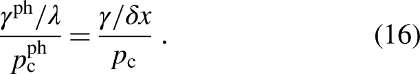
Regarding the unit conversion for the surface tension, it is important to establish the appropriate connection between the physical length scale and the lattice spacing when the interfacial properties are critical. In recent studies, Huang et al.^21,29 demonstrated that PP fluids with curved interfaces are consistent with the Laplace–Young and Kelvin equations for a $\beta$ -tuned interaction force ( ${\mathbf{F}}_{\mathrm{f}-\mathrm{f}}^{\beta }$ ) (equation 13). Accordingly, they^21,29 proposed the following similarity principle to connect the intrinsic physical length scale ( $\lambda$ ) of the lattice spacing ( $\delta x$ ) in the PP–LB:

$$\frac{{\gamma }^{\mathrm{ph}}/\lambda }{p_{\mathrm{c}}^{\mathrm{ph}}}=\frac{\gamma /\delta x}{p_{\mathrm{c}}}.$$

(16)

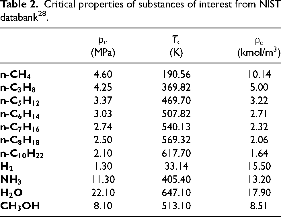
The intrinsic length scale in physical units, $\lambda$ , and the lattice spacing in lattice units, $\delta x$ , are considered equivalent as long as they yield the same dimensionless surface tension. Thus, a linear least-squares fit for $\lambda$ was carried out for the dimensionless interfacial tension (equation 16) to determine the equivalent physical length scale of $\delta x$ . The critical properties of the substances of interest are listed in Table 2.

Table 2.

Critical properties of substances of interest from NIST databank ²⁸ .

	$p_{\mathrm{c}}$	$T_{\mathrm{c}}$	${\rho }_{\mathrm{c}}$
	(MPa)	(K)	(kmol/m ${}^3$ )
n- $\mathbf{C}{\mathbf{H}}_{\mathbf{4}}$	4.60	190.56	10.14
n- ${\mathbf{C}}_{\mathbf{3}}{\mathbf{H}}_{\mathbf{8}}$	4.25	369.82	5.00
n- ${\mathbf{C}}_{\mathbf{5}}{\mathbf{H}}_{\mathbf{12}}$	3.37	469.70	3.22
n- ${\mathbf{C}}_{\mathbf{6}}{\mathbf{H}}_{\mathbf{14}}$	3.03	507.82	2.71
n- ${\mathbf{C}}_{\mathbf{7}}{\mathbf{H}}_{\mathbf{16}}$	2.74	540.13	2.32
n- ${\mathbf{C}}_{\mathbf{8}}{\mathbf{H}}_{\mathbf{18}}$	2.50	569.32	2.06
n- ${\mathbf{C}}_{\mathbf{10}}{\mathbf{H}}_{\mathbf{22}}$	2.10	617.70	1.64
${\mathbf{H}}_{\mathbf{2}}$	1.30	33.14	15.50
$\mathbf{N}{\mathbf{H}}_{\mathbf{3}}$	11.30	405.40	13.20
${\mathbf{H}}_{\mathbf{2}}\mathbf{O}$	22.10	647.10	17.90
$\mathbf{C}{\mathbf{H}}_{\mathbf{3}}\mathbf{O}\mathbf{H}$	8.10	513.10	8.51

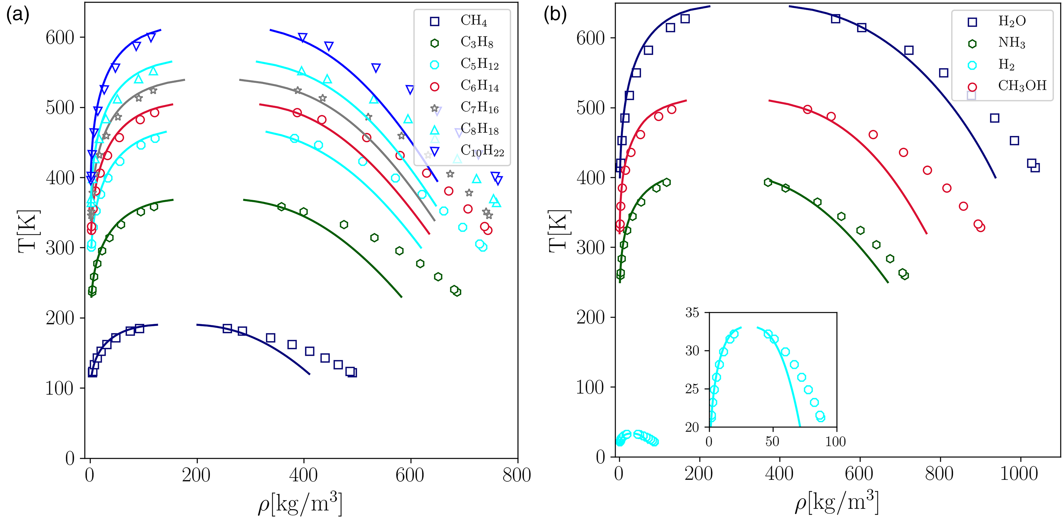
By comparing the VLE coexistence curve predicted by PP–LB in physical units with the experimental equilibrium densities from the NIST Databank ²⁸ , it is found that the PP–LB model using PR EOS fails to reproduce accurately the experimental equilibrium density branches (see Figure 5(a) and (b)), and the error increases rapidly at low reduced temperatures for all compounds. The average error for the vapor phase ( ${\mathbf{E}}_{{\rho }_{\mathrm{v}}}$ [%]) is around 10%, except for $\mathrm{C}{\mathrm{H}}_3\mathrm{OH}$ and ${\mathrm{H}}_2\mathrm{O}$ , whose ${\mathbf{E}}_{{\rho }_{\mathrm{v}}}$ is around 28%.

Figure 5.

Comparison between the experimental data and the properties predicted by the pseudopotential lattice–Boltzmann (PP–LB) method for different fluids. (a)-(b) Equilibrium densities. Experimental data ²⁸ (solid lines); LB (markers).

Figure 6.

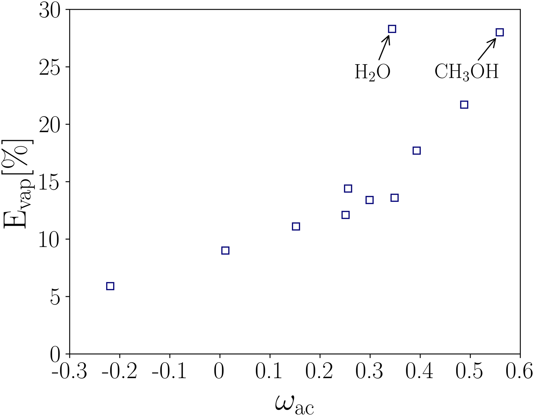
Average error for the predicted vapor phase density as a function of the acentric factor.

A monotonically increasing behavior is observed in ${\mathbf{E}}_{{\rho }_{\mathrm{v}}}$ as ${\omega }_{\mathrm{ac}}$ is raised, suggesting that the PR EOS fails to predict accurately the thermodynamic variables at all temperatures for compounds with large ${\omega }_{\mathrm{ac}}$ , regardless of the substance polarity. Meanwhile, it is also found that the percentage of ${\mathbf{E}}_{{\rho }_{\mathrm{v}}}$ drastically increases for the polar substances with OH ${}^{-}$ radical that were considered (water and methanol). As mentioned above, such deviations are directly associated with the EOS, which was reported previously by Stryjek and Vera^30,31.

Considering that the PP–LB is able to accurately reproduce the analytical thermodynamic state given by the PR equation, but fails to match the experimental VLE coexistence curve, it is suggested that the discrepancies are closely related to the choice of the EOS. Although the PR EOS that incorporates the Stryjek–Vera modifications (PRSV) and (PRSV2)^30,31 can be implemented in the PP–LB model and may be beneficial to improve the prediction of the actual behavior of the thermodynamic pressure, it may be insufficient to estimate accurately the equilibrium densities, and thus predict the proper behavior of the density ratio as a function of temperature, which is of significant interest for modeling thermal multiphase flows. Therefore, further modifications to the PR parameters may be needed ³² . Ultimately, the implementation of a more advanced EOS, such as the cubic plus association or statistical association fluid theory, may be expected to alleviate the observed inaccuracies.

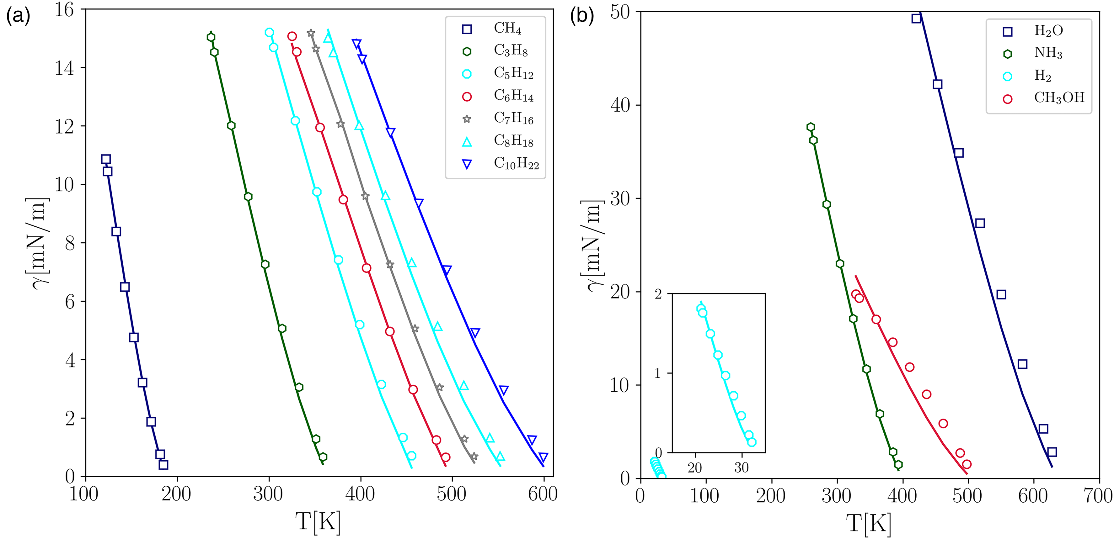
As for the determination of the surface tension ( $\gamma$ ), first the pressure difference between the liquid and the vapor phase ( $\mathrm{\Delta }p$ ) was computed for different droplet radii ( $R$ ). Next, $\gamma$ was determined by computing the slope of the Laplace–Young relation ( $\mathrm{\Delta }p=\gamma /\mathrm{\Delta }R$ ). Subsequently, ${\gamma }^{\mathrm{ph}}$ was determined through equation 16 and a least-squares linear fit for the length scale ( $\lambda$ ). Figure 7(a) and (b) compare the surface tension values obtained by PP–LB with the experimental ones, exhibiting a good level of agreement. For most of the fluids under consideration, the average error ( ${\mathbf{E}}_{\gamma }$ ) did not exceed 6%, except for ${\mathrm{H}}_2$ and ${\mathrm{H}}_2\mathrm{O}$ whose ${\mathbf{E}}_{\gamma }$ were 17.1% and 10.7%, respectively.

Figure 7.

Comparison between the experimental data and the properties predicted by the pseudopotential lattice–Boltzmann (PP–LB) method for different fluids. (a)-(b) Surface tension. Experimental data ²⁸ (solid lines); LB (markers).

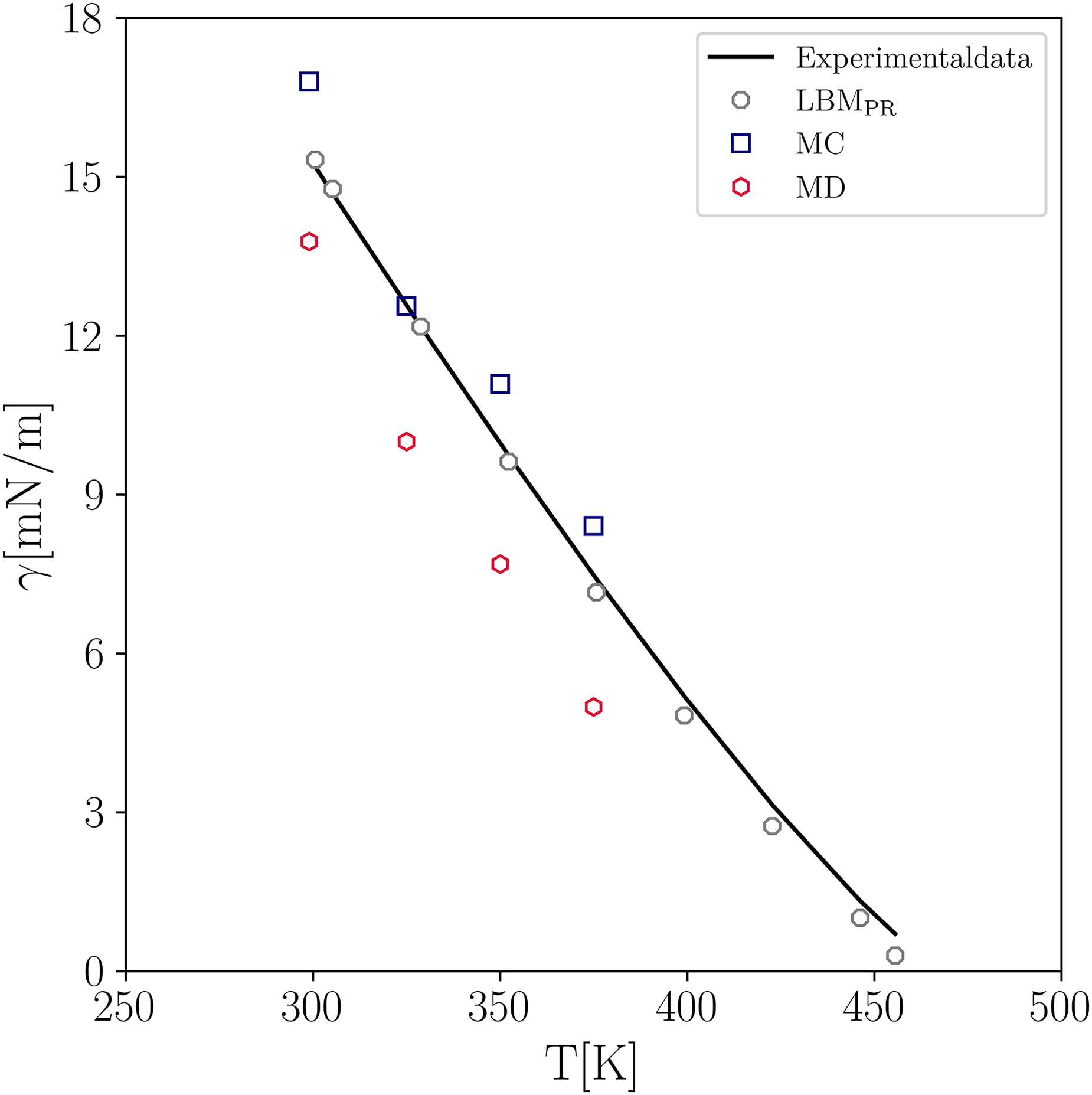
To examine the performance of PP–LB in predicting surface tension against microscale methods such as MC and MD, in Figure 8 the results obtained for C ${}_5$ H ${}_{12}$ are compared with those of Goujon et al. ³³ , who reported deviations for MC and MD of 7.5% and 24%, respectively, when considering a temperature range between 300 K and 375 K. It is clearly seen that the present PP–LB simulations closely follow the experimental values and yield a lower average error of 6.2% for a wider range of temperatures. This demonstrates the capability and versatility of LB in determining the properties of real fluids at a wide range of conditions.

Figure 8.

Comparison of predicted surface tension of pentane by MD, MC, and LB simulations. Experimental data (solid line); simulation results (markers). The MD and MC data are taken from Goujon et al. ³³ MC: Monte–Carlo; MD: molecular dynamics; LB: lattice–Boltzmann.

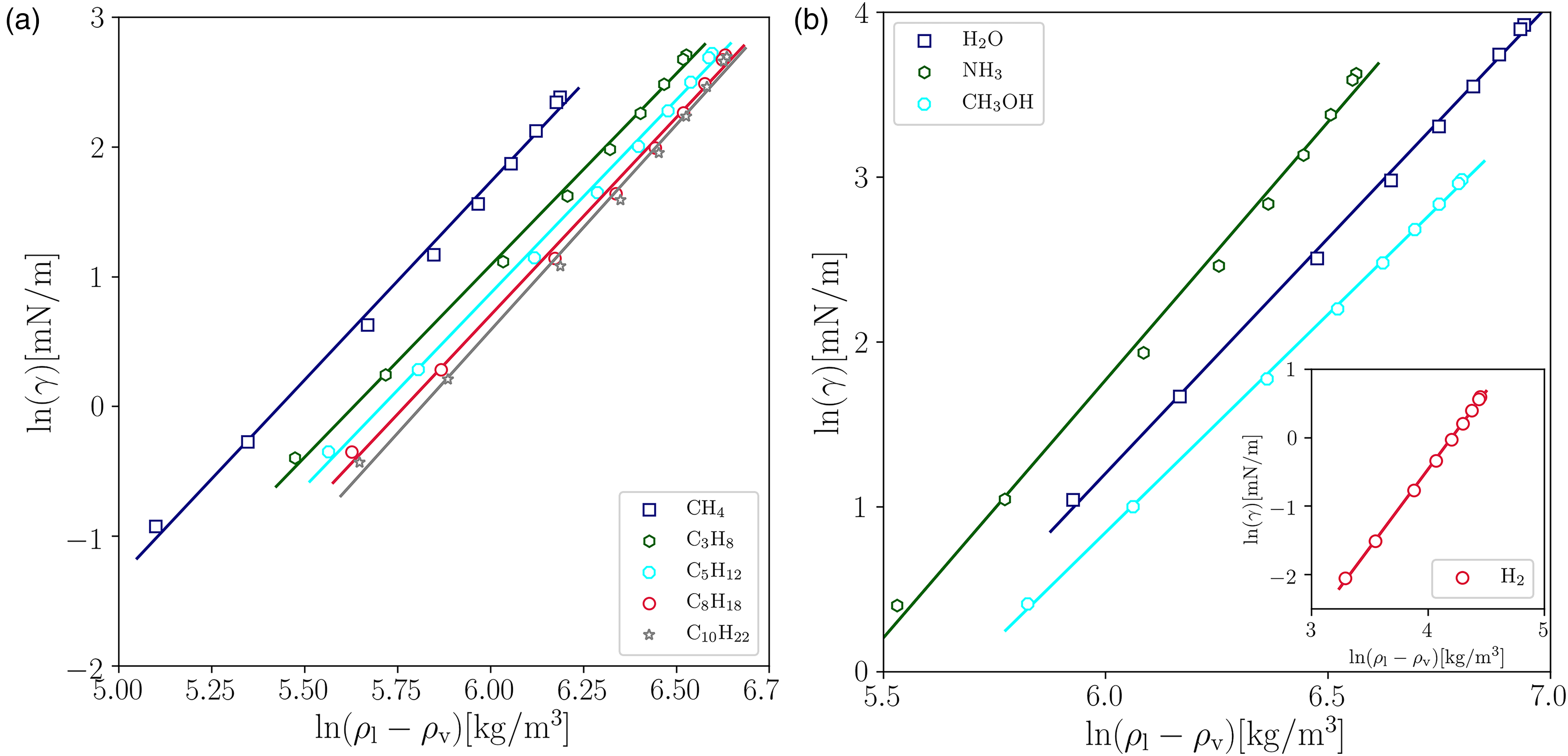
Furthermore, the thermodynamic consistency of the PP–LB was assessed by checking if the LB results satisfy the power law between $\gamma$ and $\mathrm{\Delta }\rho$ , according to the parachor model $(\mathrm{\Delta }\rho =(M/P){\gamma }^{1/4})$ , where $\mathrm{\Delta }\rho$ is computed as the difference between ${\rho }_{\mathrm{l}}$ and ${\rho }_{\mathrm{v}}$ , with $M$ and $P$ being the molar mass and parachor, respectively. In Figure 9 the linearized parachor model is plotted. For brevity, only five of the n-alkanes are presented (Figure 9(a)), as well as water, ammonia, and methanol (Figure 9(b)). It is clear that the results obtained by the PP–LB follow a linear trend, proving that they satisfy the parachor model.

Figure 9.

Power-law parachor model plot for (a) n-alkanes, as well as (b) hydrogen, water, ammonia, and methanol.

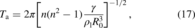
Lastly, to assess the accuracy of the model under transient conditions, an oscillating elliptical droplet was simulated. To induce the oscillatory behavior, a spherical droplet was perturbed from its equilibrium. For this test case, an ellipsoidal water droplet ( ${\omega }_{\mathrm{ac}}$ = 0.344) with major radius ( $R_{\max }$ ) and minor radius ( $R_{\min }$ ) of 34.64 and 30, respectively, was located at the center of a 200 by 200 fully periodic computational domain. To simulate the droplet dynamics in realistic conditions, we ensured that the density ratio ( ${\rho }^{*}$ ), and kinematic viscosity ratio ( ${\nu }^{*}$ ) in the lattice space were the same as those of a real water/air system. The reduced temperature was fixed at $T_{\mathrm{r}}=0.595$ , which corresponds to a density ratio close to ${\rho }^{*}$ = 1000. The analytical solution for the oscillation period of a 2D droplet is given by the following relation ³⁴ :

$$T_{\mathrm{a}}=2\pi {[n(n^2-1)\frac{\gamma }{{\rho }_{\mathrm{l}}{R}_0^3}]}^{-1/2},$$

(17)

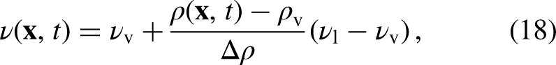
where $T_a$ is the oscillation period and $n=2$ for an elliptical droplet. The equilibrium droplet radius, $R_0$ , is given by $R_0=\sqrt{R_{\max }{R}_{\min }}$ . The following linear relation was also implemented to determine the kinematic viscosity for each phase according to the local density $\rho (\mathbf{x},t)$ :

$$\nu (\mathbf{x},t)={\nu }_{\mathrm{v}}+\frac{\rho (\mathbf{x},t)-{\rho }_{\mathrm{v}}}{\mathrm{\Delta }\rho }({\nu }_{\mathrm{l}}-{\nu }_{\mathrm{v}}),$$

(18)

and the kinematic viscosity ratio, defined as ${\nu }^{*}$ = ${\nu }_{\mathrm{v}}$ / ${\nu }_{\mathrm{l}}$ , was set equal to 15, which is close to the kinematic viscosity ratio air/water at room temperature ${\nu }_{\mathrm{air}/{\mathrm{H}}_2\mathrm{O}}=15.025$ . Thus, for the chosen ${\rho }^{*}$ = 1000 and ${\nu }^{*}$ = 15, the dynamic viscosity ratio, ${\mu }^{*}={\mu }_{\mathrm{v}}/{\mu }_{\mathrm{l}}$ , is 0.015, which is close to the air-water dynamic viscosity ratio ${\mu }_{\mathrm{air}}/{\mu }_{{\mathrm{H}}_2\mathrm{O}}\approx 0.018$ .

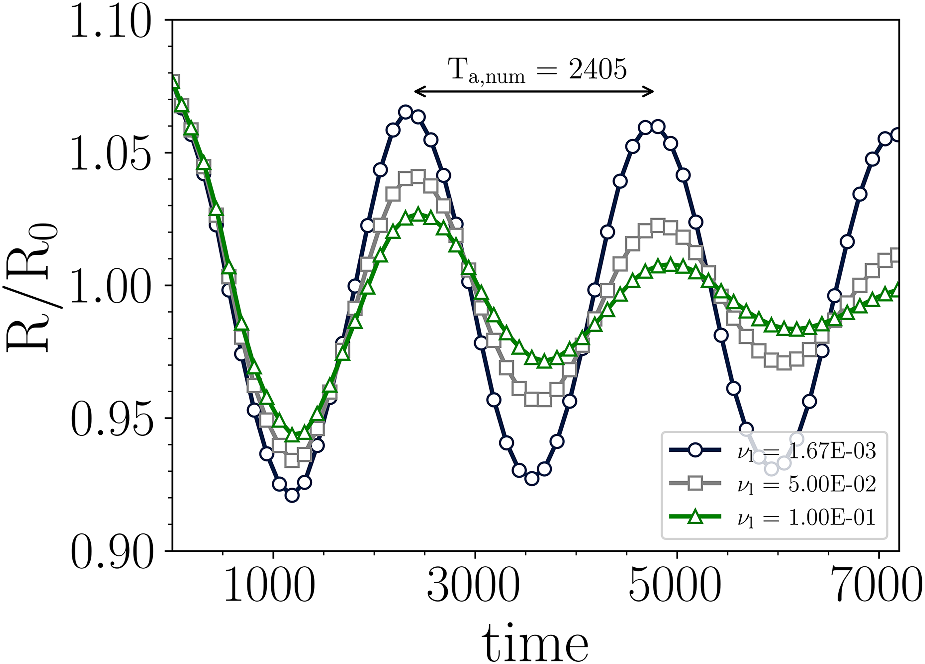
Taking advantage of the numerical stability achieved by the combination of schemes of the present work (EDM + $\beta$ -scheme + eighth-order isotropic interaction force), we were able to simulate ellipsoidal oscillating droplets at high-density ratio and remarkably low liquid viscosity up to $3.33\times {10}^{-4}$ , which corresponds to ${\tau }_{{\nu }_{\mathrm{l}}}$ = 0.501 (close to the 0.5 numerical limit). In Figure 10, the transient evolution of the normalized droplet interface, R/R ${}_0$ , is shown against the lattice time for three different liquid kinematic viscosities, ${\nu }_{\mathrm{l}}=1.67\times {10}^{-3}$ , ${\nu }_{\mathrm{l}}=0.05$ , and ${\nu }_{\mathrm{l}}=0.1$ . As can be observed, the amplitude of the oscillation is directly influenced by the droplet viscosity, which is expected and consistent with previous results ¹⁹ . In addition, the period of oscillation is accurately predicted in comparison with the analytical solution ( $T_{\mathrm{a}}\approx 2396.1$ ), obtaining $T_{\mathrm{a},\mathrm{num}}=2405$ from the simulation, which translates into a deviation smaller than 0.4%. This result demonstrates the reliability of the PP–LB to predict unsteady multiphase behavior at high-density ratios.

Figure 10.

Time evolution of oscillating ellipsoidal droplet for three different liquid viscosities.

Conclusions

The thermodynamic consistency of the multiphase PP–LB method was assessed for different substances, including linear hydrocarbons (up to C ${}_{10}$ ), ammonia, methanol, hydrogen, and water. It was shown that the LB method can be implemented to simulate multiphase flows, accurately predicting the theoretical co-existence curve given by the PR EOS for a wide range of acentric factors, raging from $-$ 0.219 to 0.559. However, the predicted equilibrium densities strongly deviate from the experimental equilibrium densities, showing that the standard PR EOS is limited for predicting the thermodynamic state of real fluids. Additionally, the physical behavior of the surface tension for a variety of substances, including both organic and inorganic compounds, was easily retrieved from the LB results, agreeing with the experimental data. Finally, it was shown that the PP–LB model is thermodynamically consistent with the parachor model and predicts accurately the transient behavior of oscillating droplets.