Sage Journals: Discover world-class research

Abstract

In this work we present a parsimonious set of ordinary differential equations (ODEs) that describes with satisfactory precision the linear and non-linear dynamics of a typical laminar premixed flame in time and frequency domain. The proposed model is characterized by two ODEs of second-order that can be interpreted as two coupled mass-spring-damper oscillators with a symmetric, nonlinear damping term. This non-linear term is identified as function of the rate of displacement following $x^{2} \dot{x}$ . The model requires only four constants to be calibrated. This is achieved by carrying out an optimization procedure on one input and one output broadband signal obtained from high-fidelity numerical simulations (CFD). Note that the Transfer Function (FTF) or describing function (FDF) of the flame under investigation are not known a-priori, and therefore not used in the optimization procedure. Once the model is trained on CFD input and output time series, it is capable of recovering with quantitative accuracy the impulse response of the laminar flame under investigation and, hence, the corresponding frequency response (FTF). If fed with harmonic signals of different frequency and amplitude, the trained model is capable of retrieving with qualitative precision the flame describing function (FDF) of the studied flame. We show that the non-linear term $x^{2} \dot{x}$ is essential for capturing the gain saturation for high amplitudes of the input signal. All results are validated against CFD data.

Keywords

Thermoacoustics non-linear flame dynamics coupled oscillators grey-box model identification ordinary differential equations

Introduction

Combustion instability remains a problem of concern during operation of gas turbines, specially when operating conditions are associated with lean premixed combustion (Lieuwen and Yang¹; Poinsot²). In order to mitigate this problem, it is of high interest to develop models and computational techniques that permit the prediction of this phenomenon at early stages of design. Hybrid approaches are the most common way to tackle combustion instability modelling. In these approaches the description of the flame response to flow fluctuations is accounted for separately from the generation of acoustic waves by the flame. The modelling of the flame response and acoustics are subsequently integrated in a single low-order model framework, usually a linearised wave equation or an acoustic network model, where the thermoacoustic stability of the system is evaluated. Furthermore, if the flame response model is non-linear in the amplitude of the incoming perturbations, such a framework is capable of predicting not only the stability but also features of the limit cycle associated with the coupling of the flame with the flow.

The Flame Describing Function (FDF) is an established non-linear flame response modelling technique (Dowling³; Noiray et al.⁴), which assumes that the flame responds at the same frequency of the input signal even if the latter exhibits large amplitudes. Therefore, an FDF is an appropriate model for weakly non-linear systems, where no interaction (flow of energy) between different frequencies is expected. The FDF can be understood as a collection of Flame Transfer Functions (FTFs) defined in the frequency domain by a gain and phase description of the system. In the FDF framework, each FTF is associated with a well defined amplitude of the input signal. Although of high relevance, the FDF is limited by the strong assumption of weakly non-linearity. Accordingly, it is only expected to satisfactorily describe flames, whose response occurs predominantly at the fundamental frequency of the input, i.e. where harmonics are negligible. In that respect, the studied limit cycles are very simple as they exhibit one single characteristic frequency. Lately Haeringer et al.⁵, introduced the concept of an extended FDF (xFDF), which includes additional transfer functions that relate higher harmonics of the output to the input. It becomes then possible to account for a response also in the harmonics and, thus, the prediction of limit cycles exhibiting more than one characteristic frequency if coupled with an acoustic model.

Once the xFDF model is available – usually obtained via harmonic forcing, where the gain and phase response of the system is calculated for each frequency and amplitude of interest – it can be used to study the dynamics of non-linear systems. Unfortunately, the xFDF models are limited as they are conceived fundamentally for harmonic signals as inputs. If coupled with a low-order model of the system acoustics and used in time domain, additional tedious calculations become necessary as the instantaneous amplitude and frequency of the incoming input signal is required. In order to overcome such a difficulty Ghirardo et al.⁶, introduced a technique, based on Hammerstein models and Fourier-Bessel series, to map the FDF from frequency to time domain via a state-space model. It was shown that such a model can reproduce well the information contained in the FDF within a narrow frequency band.

Recently, a different modelling strategy was introduced for the modelling of the non-linear flame response in the time domain (Tathawadekar et al.⁷). The derived model is obtained relatively easy from data and is more general than the FDF as it accounts for interaction between frequencies. This data-driven model, which makes use of artificial neural networks (ANN) with a rather simple multi-layer perceptron architecture, is capable of predicting the output time series given a broadband input signal that exhibits a wide frequency bandwidth and a large amplitude distribution. If desired, the trained ANN model can retrieve the FDF if excited with monofrequent signals at well defined amplitudes. Unfortunately, a trained ANN model remains obscure – it is hard to make a physical interpretation of it – and can be used only as a black-box.

Another kind of non-linear flame response models exist (Campa and Juniper⁸; Noiray and Schuermans⁹; Noiray¹⁰), that allow an interpretation of the physics involved during the evolution of limit cycles. These models describe the output of the flame response as a non-linear function of the input, usually polynomials or saturation functions, and often characterize the response as instantaneous: no time-lag is considered in the model.

Lately, some models have been proposed to account for a given characteristic time lag in the flame response (Bonciolini et al.¹¹; Gant et al.¹²). Although this kind of models is powerful if combined with low-order models of the thermoacoustic system, usually in terms of linear oscillators, they remain descriptive but not predictive as they require tuning parameters that are obtained from the same data used in the analysis.

The present study proposes a different route for the non-linear flame response modelling in the time domain. It is in part inspired by the work of Dowling³, where perturbations of the normalized heat release rate ${\dot{Q}}^{'}$ (output) are related to normalized velocity fluctuations at a reference position $u^{'}$ (input) by a linear, first order differential equation (ODE) applied to ${\dot{Q}}^{'}$ – to emulate a low-pass filter behaviour – and a non-linear function applied to $u^{'}$ – to emulate saturation. Instead of a one-dimensional ODE, we propose a two dimensional second-order ODE model that relates $u^{'}$ to ${\dot{Q}}^{'}$ to model not only the low pass filter behaviour of typical premixed flames but also local maxima and minima in the gain response. Instead of adding a nonlinear saturation function to the input $u^{'}$ , we introduce a nonlinear term into the ODEs to account for a non-linear dynamic saturation. By doing so, we dissociate ourselves from Wiener-Hammerstein models, which are characterized by simple static non-linearities.

The proposed dynamic model is capable of reproducing with reasonable accuracy the output signal given an input broadband signal with a significant amplitude and frequency distribution. If excited with mono-frequent signals at well defined amplitudes, the model is capable of retrieving the qualitative behaviour of a typical FDF, which should exhibit a low-pass filter behaviour with gain saturation for large amplitudes, and a well defined low-frequency limit.

The study is organized as follows: Starting with a Model Description, we introduce the general model equations and our motivation for using them. In the Method section we illustrate the specific case analyzed, hereby resulting in simplifications of the general model structure as well as the data used. A brief discussion of the results is done in the Results and Analysis section followed by a Conclusion and Outlook.

Model description

Mathematical motivation

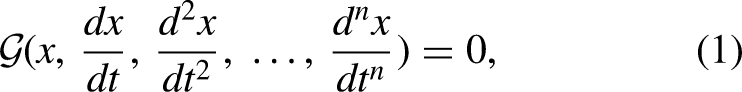
The dynamics of any time invariant system can be described by

G (x, \frac{d x}{d t}, \frac{d^{2} x}{d t^{2}}, \dots, \frac{d^{n} x}{d t^{n}}) = 0,

(1)

where

x (t)

represents a state of the system and

G

is a general function representing an autonomous, nonlinear ODE. Consider now a system bounded at all times for any combination of the arguments of

G

. Such a nonlinear function

G

is analytic and can be expanded as

\sum_{m = 1}^{M} \prod_{l = 1}^{M} (a_{m, l, 0} x + a_{m, l, 1} \frac{d x}{d t} + \dots + a_{m, l, n} \frac{d^{n} x}{d t^{n}}) = 0.

(2)

Equation (2) describes the dynamics of bounded, time invariant systems – typical features of systems in nature – and is therefore general. In the present work we aim at simplifying Eq. (2) by retrieving essential features via physical analysis.

Physical motivation

Figure 1 illustrates a typical heat release rate response of a premixed flame to an impulse of upstream velocity. As seen in this example, a characteristic flame impulse response exhibits - after some initial time delay - a strong positive peak usually followed by further peaks of alternating sign and decreasing amplitudes. Such a response reflects the oscillating behaviour of the flame surface area as the flame reacts to an impulse of velocity at its base. This oscillating behaviour is remarkably similar to the one of a simple mass-spring-damper system – a classical second-order ODE referred in this work as oscillator.

Figure 1.

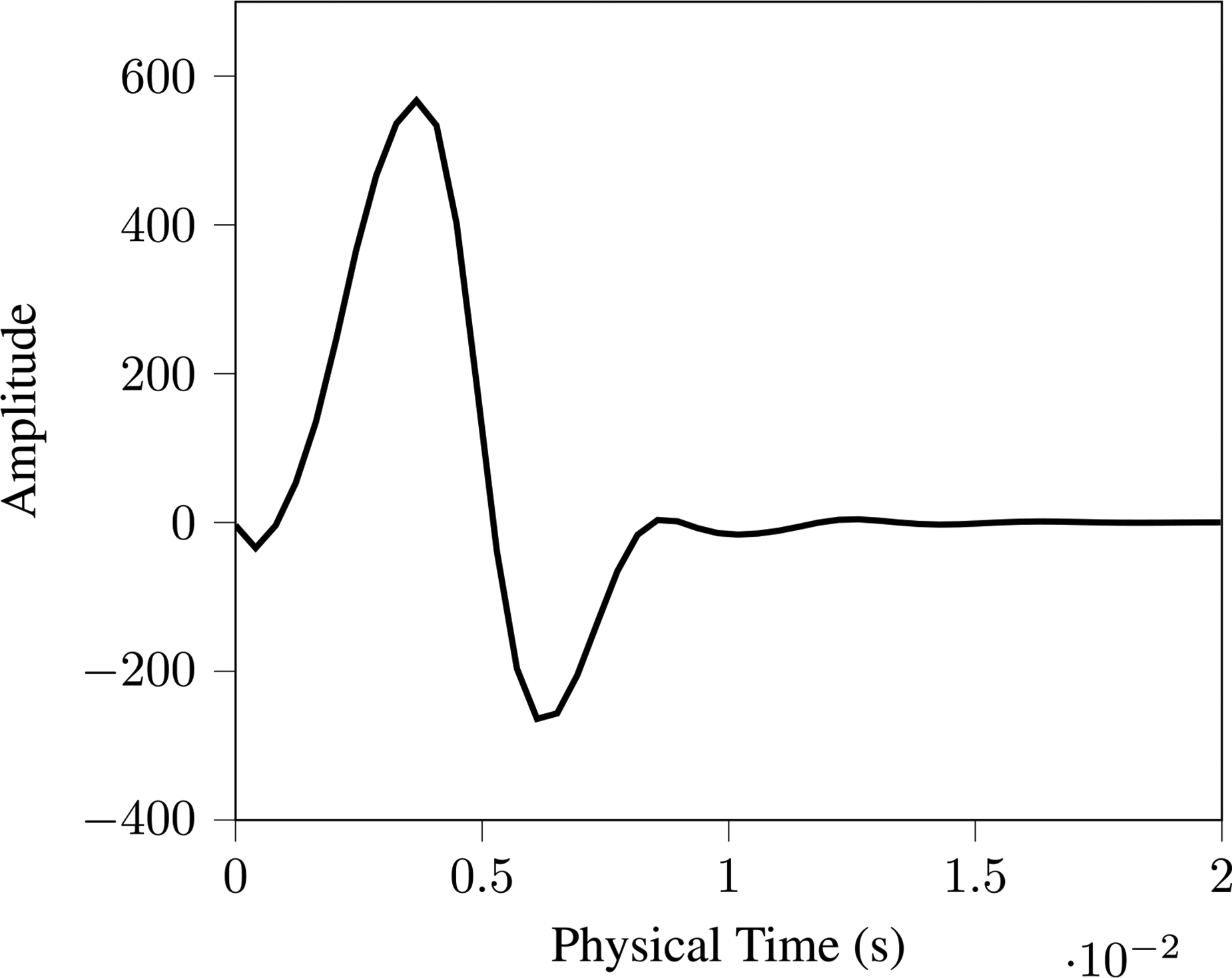
Flame impulse response of a laminar slit burner configuration (Silva et al.¹³).

Compared to a single-mass oscillator, a real flame exhibits much richer dynamics. Individual flame regions may react differently to external excitation. The response of e.g. flame foot and flame tip may interfere constructively or destructively. Such a behaviour cannot be captured by a single second order ODE as we require more than two dimensions. In this work we show that two coupled oscillators can already capture very well the dynamics of a typical slit flame. Naturally, more complex flames, such as turbulent swirled flames, may require additional dimensions.

The physical significance of the proposed oscillator model, which is likely related to flame-flow feedback mechanisms, is not immediately obvious. While the mass(es) can be interpreted as flow inertia, the physical meaning of springs and dampers remains hidden. Note, however that an (isolated) flame, in the same way as an oscillator, has a stable equilibrium position, to which it eventually returns after a given perturbation. Thus, there exist a restoring force (spring) which is a function of displacement and a damping force (damper), which is a function of the rate of displacement.

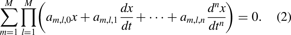
In the present study, we do not aim at finding physical correspondence for the individual model components. Instead, we employ the proposed model as a demonstration that a very simplified version of Eq. (2), which represents very well the flame dynamics of a slit flame, can be inferred by simple analysis. The obtained two-coupled oscillators model could be exploited to investigate the flame response with an analogous mechanical model. The interpretation of the model components (nonlinear springs and dampers) remains a task of interest for future work.

General model equations

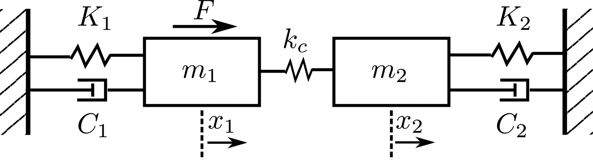
We start by proposing the horizontal, two-degrees of freedom mass-spring-damper oscillator model depicted in Figure 2. As we rely on a small number of dimensions, we use Newton’s notation for time derivative $d x / d t = \dot{x}$ . Both masses are attached to a neighbouring wall via a spring and a damper with possibly non-linear characteristics $K_{1 / 2} (x_{1 / 2}, {\dot{x}}_{1 / 2})$ and $C_{1 / 2} (x_{1 / 2}, {\dot{x}}_{1 / 2})$ . The masses are coupled via a third spring with linear stiffness $k_{c}$ . Depending on the functional form of spring and damper characteristics $K_{1 / 2}$ and $C_{1 / 2}$ , the resulting model will be linear or non-linear.

Figure 2.

Coupled mass-spring-damper oscillator system representing the ODE system proposed in this work.

The input (i.e. normalized velocity fluctuations $u^{'}$ ) is represented as a horizontal force $F$ , acting on the first mass $m_{1}$ . The position $y = x_{2} (t)$ of the second mass $m_{2}$ is selected as output, and represents the normalized heat release rate fluctuation ${\dot{Q}}^{'}$ . Assuming that at $t = t_{0}$ both masses are at their equilibrium position $x_{1} (t_{0}) = 0$ and $x_{2} (t_{0}) = 0$ , the model equations write

\begin{aligned} m_{1} {\ddot{x}}_{1} = F - C_{1} (x_{1}, {\dot{x}}_{1}) {\dot{x}}_{1} - K_{1} (x_{1}, {\dot{x}}_{1}) x_{1} + k_{c} (x_{2} - x_{1}) \end{aligned}

(3)

m_{2} {\ddot{x}}_{2} = - C_{2} (x_{2}, {\dot{x}}_{2}) {\dot{x}}_{2} - K_{2} (x_{2}, {\dot{x}}_{2}) x_{2} - k_{c} (x_{2} - x_{1})

(4)

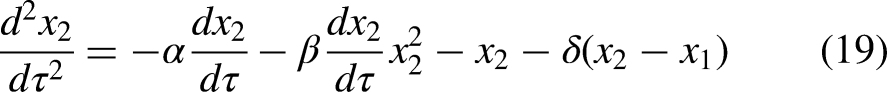
Non-linear contributions

The functional form of the non-linear spring and damper characteristics governs the non-linear dynamics of the oscillator model and is thus decisive for the achievable match with the observed flame dynamics. Assuming that the spring and damping forces acting on the two masses are smooth functions of $x$ and $\dot{x}$ , they can be expanded into a Taylor series around the equilibrium point $x$ = $\dot{x}$ =0. Considering terms up to order three yields a general non-linear spring force $F_{k} = K (x, \dot{x}) x$ and damping force $F_{c} = C (x, \dot{x}) \dot{x}$ according to

F_{k} = (k + l x + m {\dot{x}}^{2} + n x^{2}) x

(5)

F_{c} = (c + d x + e \dot{x} + f x^{2} + g {\dot{x}}^{2}) \dot{x}

(6)

The uni-variate even terms in Eq. (5) and Eq. (6) result in an undesired non-zero mean of the model output for a general zero mean input signal. Vice versa, when prescribing a zero output mean (the output represents the de-trended normalized heat release rate), the even terms vanish, equivalent to

l = e = 0

(Bonciolini et al.¹¹; Lieuwen¹⁴). Depending on the value of

d

, the mixed second order term in Eq. (6) may cause overall negative damping, which would de-stabilize the oscillator. To avoid this issue we set

d = 0

. The uni-variate cubic term in Eq. (5) results in an amplitude dependent low-frequency limit of the in-output behaviour, which is not physical (see Sec. Low-Frequency Limit). We thus set

n = 0

According to our observations, the mixed cubic term $f x^{2} \dot{x}$ in Eq. (6) is by far the most important one among all remaining non-linear terms. In order to keep the model as simple as possible we drop the other two remaining non-linear terms by setting $m = g = 0$ . Note that these terms have no significant effect on the overall model performance for the flame investigated in this study. The retained non-linear term $f x^{2} \dot{x}$ results in increasing damping for larger amplitudes. This will reduce the gain overshoot near the resonance frequencies of the oscillator for increasing amplitudes - a phenomenon typically observed in an FDF and known as saturation.

Interestingly, this analysis yields the same non-linear contribution as obtained in previous studies (Lieuwen¹⁴;Noiray and Schuermans¹⁵; Bonciolini et al.¹¹). However, in those studies the entire thermoacoustic system is represented as a (single-mass) non-linear oscillator, and the flame dynamics is only represented by a static, nonlinear term (with or without a delay).

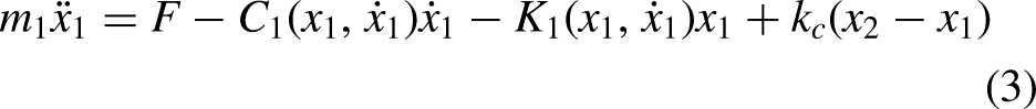
Finally, the resulting non-linear model equations are

m_{1} {\ddot{x}}_{1} = F - c_{1} {\dot{x}}_{1} - f_{1} x_{1}^{2} {\dot{x}}_{1} - k_{1} x_{1} + k_{c} (x_{2} - x_{1})

(7)

m_{2} {\ddot{x}}_{2} = - c_{2} {\dot{x}}_{2} - f_{2} x_{2}^{2} {\dot{x}}_{2} - k_{2} x_{2} - k_{c} (x_{2} - x_{1}),

(8)

where the two parameters

f_{1}

and

f_{2}

govern the non-linear dynamics of the oscillator. Equations (7) and (8) are clearly simplifications of Eq. (2), since, if combined, they amount to four dimensions with only two nonlinear terms.

Low-frequency limit

Using global conservation laws for mass, energy, and momentum Polifke and Lawn¹⁶ demonstrated that the transfer function between velocity fluctuations $\hat{u}$ and heat release rate fluctuations $\hat{\dot{Q}}$ of a perfectly premixed flame should be unity in the limit of zero frequency. Here $\hat{*}$ denotes the Laplace transform of a quantity $*$ .

F (ω = 0 ‖ \hat{u} ‖) = \frac{\hat{\dot{Q}} (ω = 0)}{\hat{u} (ω = 0)} \overset{!}{=} 1

(9)

We can easily calculate the static response by setting all time derivatives to zero. Using the previously derived model (Eqs. (7) and (8)), we obtain a constraint of the form:

\frac{k_{1} k_{2}}{k_{c}} + k_{1} + k_{2} \overset{!}{=} 1,

(10)

which relates the linear stiffnesses

k_{1 / 2}

and

k_{c}

to each other. By using this constraint, we can further reduce the amount of parameters that need to be tuned, while explicitly enforcing a known physical behaviour of the flame. Note, that a uni-variate cubic non-linearity in the stiffness (

n \neq 0

in Eq. (5)) would not allow to set the low frequency limit by a condition like Eq. (10). Instead, it would result in an amplitude-dependent low-frequency limit.

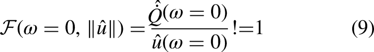
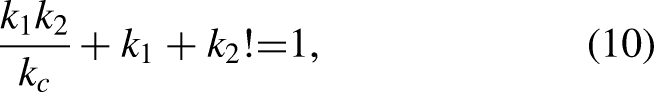
Interestingly, the approach presented in Sec. Method would satisfy the constraint presented above even without explicit consideration of the static response. Although this points to the robustness of our approach, we implement the low-frequency limit explicitly, thus reducing the number of adjustable parameters by one. The ability to incorporate physical knowledge into our system - i.e. using grey box modelling - is an advantage compared to purely data driven black-box system identification.

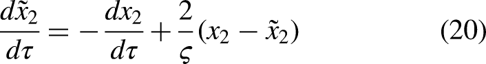
Manipulating the phase response

The system of coupled oscillators under investigation (see Eqs. (7) and (8)) is a minimum phase system. This means that there exists no system with the same gain characteristics that produces a smaller shift in phase. We desire now to make the system of coupled oscillators of non-minimum phase. That allows the direct manipulation of the phase response of the system without alteration of the gain response. In other words, the design of a non-minimum phase system gives us an additional degree of freedom for a correct phenomenological representation of the flame response. For a system to be non-minimum phase it is required that the associated transfer function exhibits at least one zero in the right-half of the complex plane (Lunze¹⁷).

Let us consider the characteristic equation of a linear, single oscillator $\ddot{x} + \dot{x} + x = u$ , where the constants are considered unity for simplicity. The phase response of such an oscillator can be manipulated by considering a pure time delay on the input as $u (t - ς)$ . The Laplace transform of the resulting expression yields

\hat{x} (s) = \frac{\hat{u} (s)}{s^{2} + s + 1} e^{- s ς},

(11)

where

s

is the Laplace variable. Figure 3(a) shows the gain and phase response of the single oscillator with and without time delay

ς

(illustrated in black and red colour, respectively). Although the model of Eq. (11) permits the manipulation of the phase by the time delay

ς

, it is difficult to introduce to standard gradient descent optimization schemes. This difficulty originates from the fact that numerical integration schemes are required to solve the system of ODEs. Regardless which scheme we choose to do so, the delay value

ς

can no longer take arbitrary continuous values from zero to infinity, but only multiples

n

of time step

Δ t

, chosen for numerical integration.

u (t - ς) ⟶ u_{k} (t_{k} - n Δ t) where n = ⌈ \frac{ς}{Δ t} ⌉

(12)

Figure 3.

$(a)$ Frequency response (Magnitude and Phase) of a single oscillator (black), with pure time delay (red) and first order Padè approximant of the time delay (blue). $(b)$ Impulse response of the three cases analyzed.

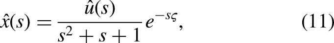
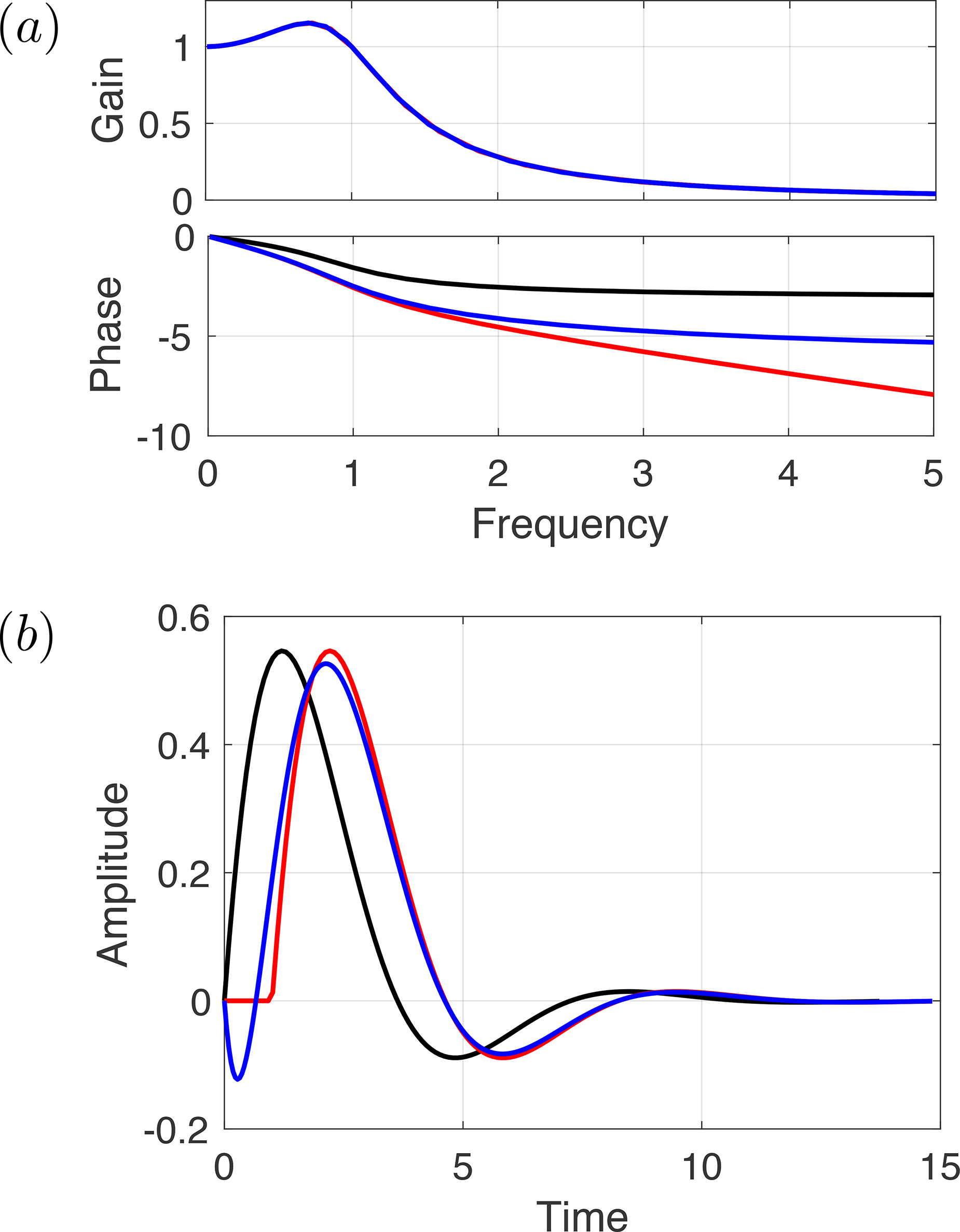
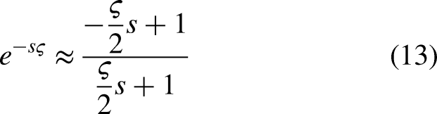
Here we denote the current integration step as $k$ with $k \in [1, 2, \dots, K]$ . Optimization of a non-continuous delay control parameter $n$ in combination with continuous model parameters (e.g. mass, spring stiffness, etc.) is not straightforward and introduces significant complexity to any optimization approach.

In order to counteract this difficulty, a Padè approximant of the exponential quantity is applied. The first order approximation reads

e^{- s ς} \approx \frac{- \frac{ς}{2} s + 1}{\frac{ς}{2} s + 1}

(13)

Replacing Eq. (13) in Eq. (11) results in

\hat{x} (s) = \frac{\hat{u} (s)}{s^{2} + s + 1} \frac{- \frac{ς}{2} s + 1}{\frac{ς}{2} s + 1},

(14)

which describes a non-minimum phase system, as it has one zero on the right-half of the complex plane at

2 / ς

. As a result, the term

(- \frac{ς}{2} s + 1) / (\frac{ς}{2} s + 1)

does not affect the gain of the system. It exclusively affects the phase response via a time delay

ς

, as illustrated in Figure 3(a) (blue line). After applying the inverse Laplace transform to Eq. (14), we obtain a formulation for the delay in the time domain, yielding:

\dot{\tilde{x}} = - \dot{x} + \frac{2}{ς} (x - \tilde{x})

(15)

where

\dot{\tilde{x}}

and

\tilde{x}

refer to the delayed value of

\dot{x}

and

x

respectively. The above equation is straight forward to implement into any numerical integration scheme allowing to control the delay via a now continuous control parameter

ς

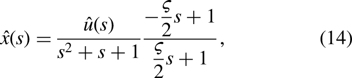
The first order Padè approximant is in good agreement with the reference case (red line) for low frequencies. Note that Eq. (14) is rational. Such a rational structure of the flame response function is ideal, when used together with acoustic network models, for studies on combustion instability because eigenvalue problems linear on the eigenvalue $s$ can be formulated. For completeness, Figure 3(b) shows the impulse response of the three cases analyzed.

In the present work, the phase response of the non-linear, coupled oscillators system, as per Eqs. (7) and (8), is manipulated by the aforementioned technique, where a time-delay is introduced in the system by a first-order Padè approximant.

Note that application of the Padè approximant introduces an initial dip in the impulse response (see Figure 5). This local minimum introduces a new additional time scale to the model response. The resulting change in model behaviour is in good agreement with the actual flame response depicted in Figure 1, which qualitatively expresses the same initial dip in its impulse response.

Figure 5.

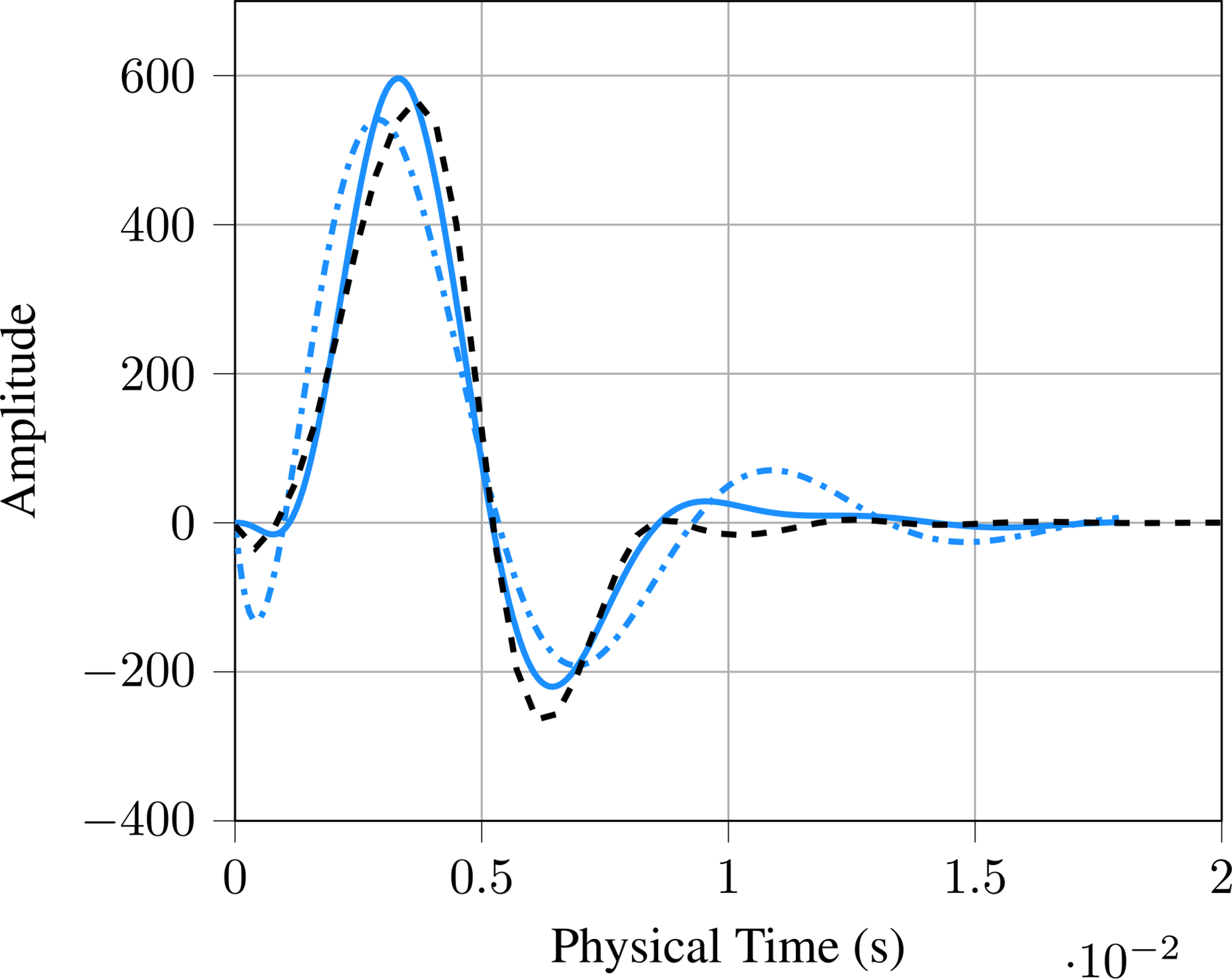
Impulse response of LDO (blue, solid) and LSO (blue, dash dotted). Both are optimized on linear time series data and compared to a reference impulse response (black, dashed) resulting from established black box system identification tools. LSO and LDO impulse response are transformed to physical time $t$ .

Method

Input and target data

During optimization, the model is presented to time series data consisting of broadband excitation data of the (normalized) fluctuations of the inlet velocity $u^{'}$ and the corresponding (normalized) fluctuations in the heat release rate of a laminar premixed flame ${\dot{Q}}^{'}$ . The model is trained on input and output time series data only. Accordingly, we do not assume to know the corresponding FTF or FDF a priori. Gain and phase data of the system under investigation are used only for validation purposes.

We investigate our model performance on two types of numerical data sets, a linear and a non-linear one. The general set-up is similar to the multi-slit Bunsen burner set-up which was investigated experimentally by Kornilov et al.¹⁸ and numerically by Silva et al.¹³ and Jaensch and Polifke¹⁹ respectively. The first data set is generated using only small input amplitudes, and is used to evaluate the linear flame response. The second data set contains larger input forcing amplitudes, and is used to evaluate the non-linear flame response. The broadband signals and their amplitude probability density function are depicted in Figure 4. For a detailed description of the numerical set up used to obtain these data sets, we refer to the works of Silva et al.¹³ and Jaensch and Polifke¹⁹.

Figure 4.

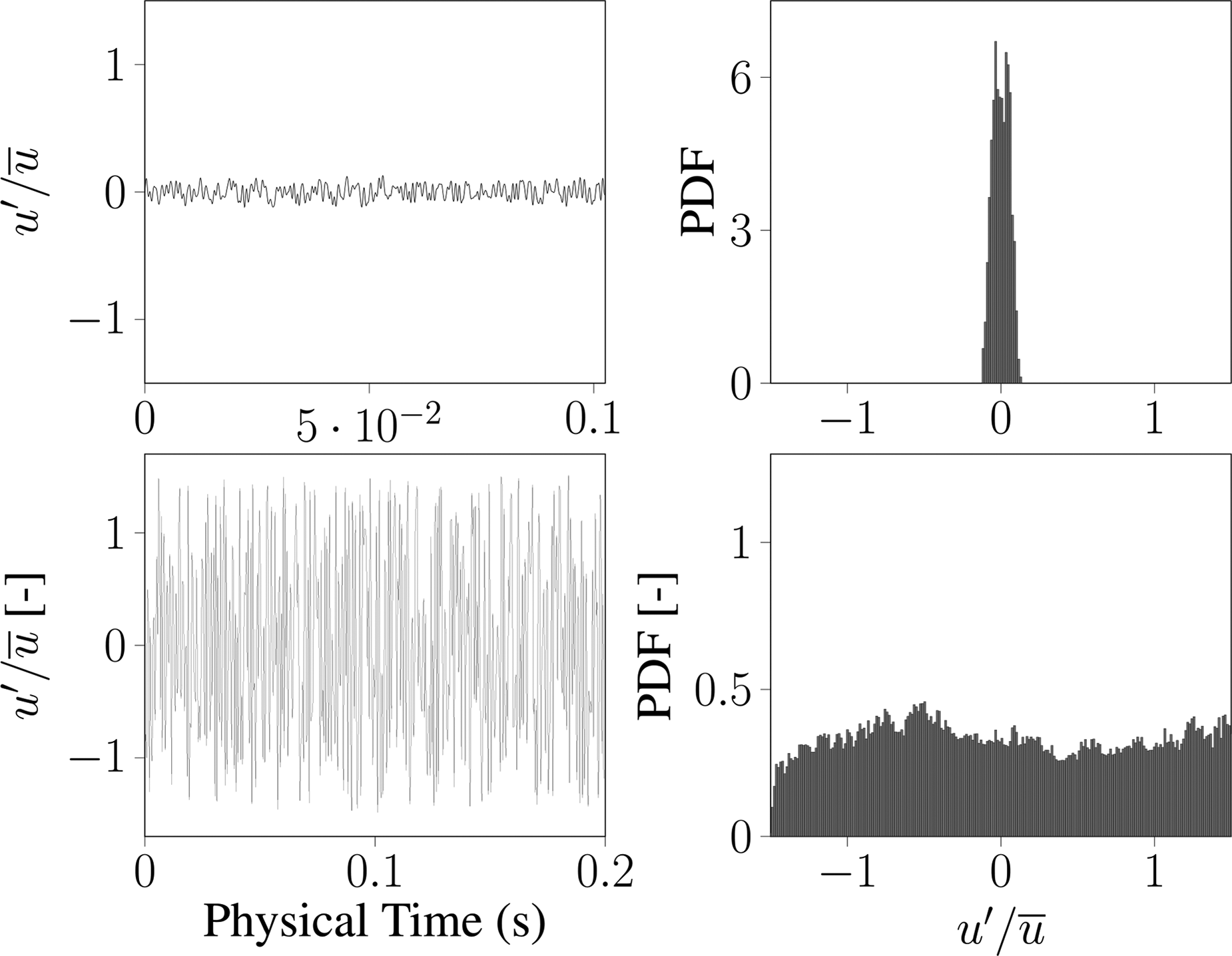
Input signals used to train the models. Linear data set on top, non-linear data set at the bottom. Left: Input time series data, Right: Probability density function (PDF) of the input data.

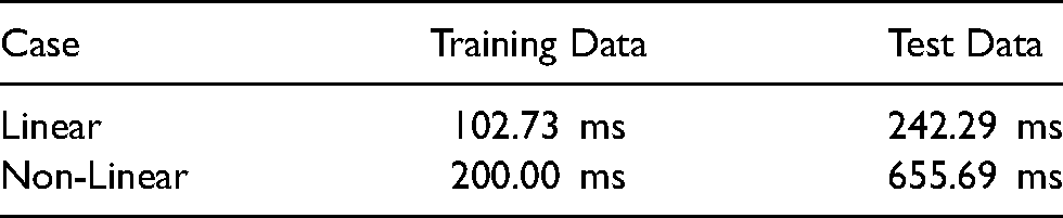
Using the same numerical set up as well as the given amplitude probability density distribution function of the input signals, a linear and a non-linear test data set are produced. Table 1 provides an overview over the signal length of each training and test signal used in this work.

Table 1.

Length of each signal in milliseconds (ms).

Case	Training Data	Test Data
Linear	102.73 ms	242.29 ms
Non-Linear	200.00 ms	655.69 ms

Time scaling of the equations

The model introduced so far assumes different physical parameters for each pendulum mass, resulting in ten parameters governing the model. As demonstrated in the Low-Frequency Limit subsection, we can reduce the number of parameters by using the constrains stated in Eq. (10). Refraining from a detailed discussion, we notice that models using a uniform parametrization (i.e. both masses share the same parameters $m$ , $k$ , $c$ and $f$ ) perform roughly equally well as more complex models, using different parameters for each mass. The minor decrease in modelling capacity is offset by the significant reduction in parameters governing the model. With a uniform parametrization and using the constraint stated by Eq. (10), we can describe the model using only five parameters.

In general, the flame responds in a time window of milliseconds. Thus, an oscillator system that is able to model such (fast) flame dynamics, can be expected to feature very small masses and very high spring stiffness values. The extremely small mass values on their own can lead to serious optimization difficulties due to finite machine precision. Furthermore, large differences (several orders of magnitude) between $k$ , $k_{c}$ and $m$ will make any gradient based optimization attempts extremely challenging. We can avoid these problems by introducing a non-dimensional time scale $τ$ . Following the procedure described by Strogatz²⁰ we write:

τ = \frac{t}{T_{ref}}

(16)

We can interpret this relation as a transformation of the flame dynamics, in a time domain where all processes occur

T_{ref}

times faster or slower, depending on whether

T_{ref}

is larger or smaller than one respectively.

We require now to find a suitable value for 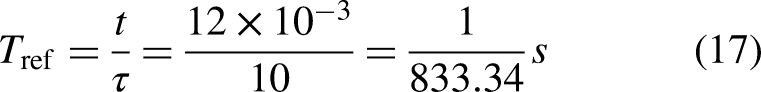$T_{ref}$ . A spring-mass-damper oscillator with stiffness, damping and mass values of order $O (1)$ exhibits an impulse response around 10 seconds long (see Figure 3). Consider this to be a characteristic value for the non-dimensional time $τ$ so that $t / T_{ref} \sim 10$ . Let us find now what is a characteristic time $t$ for the flame under investigation. We make use of the definition of restoration time, proposed by Blumenthal et al.²¹, which should be understood as the time that it takes the flame to return to its initial position after being perturbed by an impulse of velocity at its base. We calculate that time around 6 ms, following the geometrical values shown in Figure 3 of Kornilov et al.¹⁸. The impulse response of a given flame can be slightly under-damped. As a result, the flame oscillates two or three times before reaching equilibrium. In most of the cases investigated in his Thesis Steinbacher²² shows that equilibrium is recovered after approximately two times the value of the restoration time. Following these observations, we calculate a characteristic time of the impulse response to be $t = 2 \times 6$ ms $= 12$ ms. A suitable value for $T_{ref}$ is then computed as:

T_{ref} = \frac{t}{τ} = \frac{12 \times 10^{- 3}}{10} = \frac{1}{833.34} s

(17)

The flame dynamics have to be decelerated by roughly factor 833, so that the oscillator model exhibits parameter values of

O

(1). Further investigation revealed, that for a large range of

T_{ref}

, the model performance is independent from the

T_{ref}

chosen. For the case at hand, we therefore do not further optimize

T_{ref}

to keep the optimization as simple as possible. In cases, in which an initial guess of

T_{ref}

is subject to more uncertainty, the linear stage of optimization (discussed in the following subsection) can be repeated for different values of

T_{ref}

With an interpretation and value for 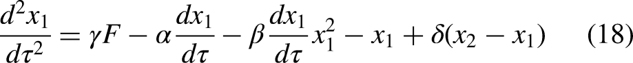$T_{ref}$ at hand, we transform the model equations by replacing the physical parameters in Eqs. (7), (8) and (15) according to Table 2 and introduce the time derivatives with respect to $τ$ .

\frac{d^{2} x_{1}}{d τ^{2}} = γ F - α \frac{d x_{1}}{d τ} - β \frac{d x_{1}}{d τ} x_{1}^{2} - x_{1} + δ (x_{2} - x_{1})

(18)

\frac{d^{2} x_{2}}{d τ^{2}} = - α \frac{d x_{2}}{d τ} - β \frac{d x_{2}}{d τ} x_{2}^{2} - x_{2} - δ (x_{2} - x_{1})

(19)

\frac{d {\tilde{x}}_{2}}{d τ} = - \frac{d x_{2}}{d τ} + \frac{2}{ς} (x_{2} - {\tilde{x}}_{2})

(20)

Table 2.

Overview of used coefficients and the respective physical parameters they comprise.

Coefficient	$α$	$β$	$γ$	$δ$	$T_{ref}$
Physical Parameters	$\frac{c}{\sqrt{m k}}$	$\frac{f}{\sqrt{m k}}$	$\frac{1}{k}$	$\frac{k_{c}}{k}$	$\sqrt{\frac{m}{k}}$

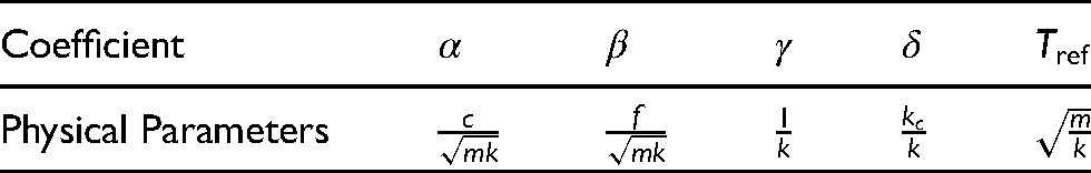
Using the definition of 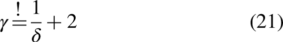$γ$ and $δ$ we can transform the constraint stated in Eq. (10) yielding:

γ \overset{!}{\frac{1}{δ}} + 2

(21)

This leaves us with four parameters

α, β, δ

and

ς

to be determined by the optimization routine.

Optimization

For optimization purposes, each data set (linear and non-linear one) is divided into a training and a test data set. The performance on the training set is used during the optimization procedure itself (e.g. to calculate a loss) while the performance on the test data is used to validate the model.

We interpret the linear oscillator model as special case of a general non-linear model, which is applicable for small input amplitudes only. Following this line of thought, our goal during optimization is to obtain a well performing linear model, which we then extend by a non-linear contribution responsible for modelling the saturation effect observed in the FDF (i.e. in the frequency domain). We thus propose a staged optimization approach. First, the non-linear contribution $β$ is set to zero and ignored by the optimizer. We obtain a linear model, by carrying out optimization on time series data from the linear data set. The resulting model corresponds in frequency domain to the FTF. Secondly, we optimize the non-linear model contribution controlled via $β$ on the non-linear data set, keeping fixed the already optimized linear parameters $α$ and $δ$ as well as the delay control parameter $ς$ .

By training linear parameters only on linear data, we avoid training the linear model contribution to dynamics only present in the non-linear data set, which would significantly worsen the model performance for small $u^{'}$ forcing amplitudes.

By doing so, we ensure the best possible model performance over a wide range of input amplitudes and forcing frequencies.

As starting point for our staged optimization chain, we require an initial guess for our parameters. We start by putting all adjustable parameters to unity.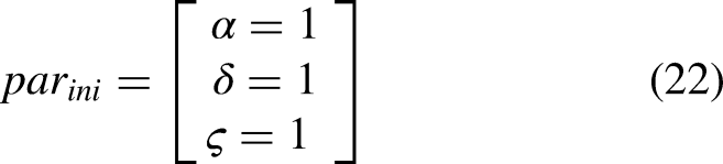

p a r_{i n i} = [\begin{matrix} α = 1 \\ δ = 1 \\ ς = 1 \end{matrix}]

(22)

Note that depending on the data at hand, setting all parameters to unity might not result in suitable initial model parametrization. In such cases, the linear optimization stage can be performed for multiple initial parametrizations, to find the most adequate one for the given data.

We use the Euclidean norm between the output of a given model and the target reference data as loss function $J$ during optimization.

J = ‖ y_{ref} - y_{m o d e l} ‖_{2},

(23)

where

y_{r e f}

and

y_{m o d e l}

represent the normalized heat fluctuations

{\dot{Q}}^{'}

of the target flame and the model prediction respectively.

The obtained values are however difficult to interpret on their own, especially when applying the model to the test data set. We thus introduce a more intuitive %-fit loss value, which is used in Table 3 presenting the final results of optimization. Please note that this value is used in post processing only and not as loss function during optimization. The %-fit value is based on the normalized root mean square error and calculated as follows: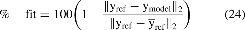

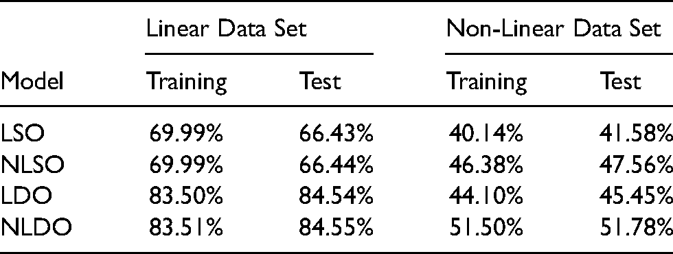
\% -fit = 100 (1 - \frac{‖ y_{r e f} - y_{m o d e l} ‖_{2}}{‖ y_{r e f} - {\bar{y}}_{r e f} ‖_{2}})

(24)

where

{\bar{y}}_{ref}

represents the mean of

y_{ref}

, a given reference output.

Table 3.

Performance values for different stages of optimization and number of oscillators on training and test set for linear and non-linear data sets.

	Linear Data Set		Non-Linear Data Set
Model	Training	Test	Training	Test
LSO	69.99%	66.43%	40.14%	41.58%
NLSO	69.99%	66.44%	46.38%	47.56%
LDO	83.50%	84.54%	44.10%	45.45%
NLDO	83.51%	84.55%	51.50%	51.78%

Table 4.

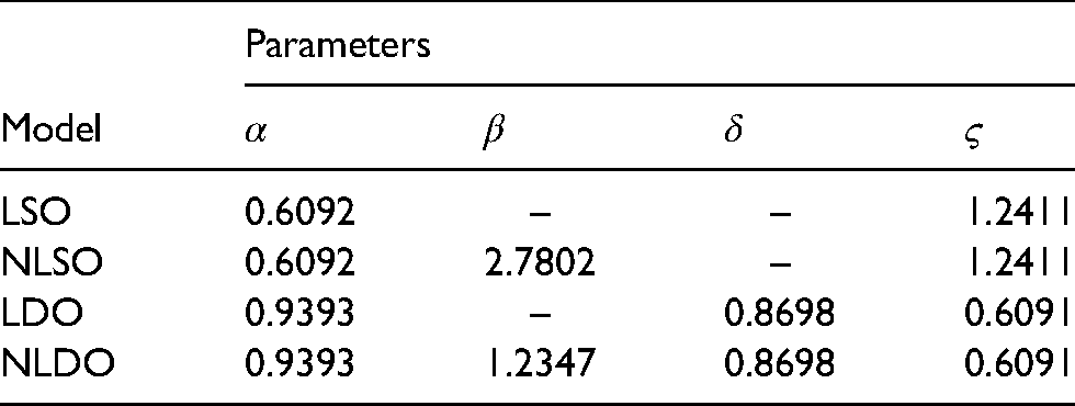
Parameters for models presented in Table 3. Note, $T_{ref}$ was set to $1 / 833.34$ s for all models

Model	Parameters
Model	$α$	$β$	$δ$	$ς$
LSO	0.6092	–	–	1.2411
NLSO	0.6092	2.7802	–	1.2411
LDO	0.9393	–	0.8698	0.6091
NLDO	0.9393	1.2347	0.8698	0.6091

For the linear as well as the non-linear stage of optimization, we use a variant of the constrained limited-memory Broyden–Fletcher–Goldfarb–Shanno (L-BFGS) algorithm, the so called L-BFGS-B algorithm (see Byrd et al.²³ for a detailed description).

As with linear parameters $α$ , $δ$ and $ς$ , the non-linear parameter $β$ is initialized to unity.

Note that we applied a time transformation when deriving model Eqs. (18) & (19). Thus, we need to transform the discrete time stepping of the input and output data according to Eq. (16).

Both stages of optimization combined take around 20 seconds of runtime on a single CPU at 3 GHz, thus runtime is not an issue.

Results and analysis

In the results presented, we differentiate between two model architectures and the two different stages of optimization. The classification is as follows:

Linear Single Oscillator (LSO)

Non-Linear Single Oscillator (NLSO)

Linear Double Oscillator (LDO)

Non-Linear Double Oscillator (NLDO)

Here, the terms linear and non-linear refer to the stage of optimization as well as the dynamics inherent to the model. Linear models are the result of linear optimization where

β = 0

, whereas non-linear models are obtained after subsequent optimization of

β

, keeping the linear parameters constant. Double models refer to the model depicted in Figure 2 and described by Eqs. (18) and (19). In order to demonstrate the need for a second oscillator mass – an additional second order ODE, a comparison against an oscillator using only a single mass is performed. We refer to this model architecture as single model. The equations describing this model can be derived from Eq. (18) by setting

δ = 0

. Since here only a single mass is used, the force is imposed to the same mass, whose position is used as output.

Results after linear optimization

We start with an analysis of the results obtained after the first stage of optimization, i.e. the non-linear $β$ contribution in the model was deactivated and the model was trained on data comprising of small input forcing amplitudes only.

Table 3 provides an overview of model performance on training and test data set for the linear and non-linear case. We analyze the %-fit value introduced by Eq. (24), with Table 4 containing the corresponding parameters. For this first part of the analysis, we focus on the performance of the LSO and LDO models. The LSO achieves a $\approx 66 %$ fit on time series test data, whereas the LDO model achieves a remarkable $\approx 85 %$ fit. The significant drop in performance when applying the linear models to the non-linear data set is to be expected and serves as motivation to add the non-linear contribution presented in the Model Description.

We have relied only on time series data for training and testing. The obtained model should properly characterize the system. It is now possible to asses its impulse response (Figure 5) and also the frequency response (Figure 6). For further (post processing) analysis, we use the impulse and frequency response data from Silva et al.¹³ as reference data for validation.

Figure 6.

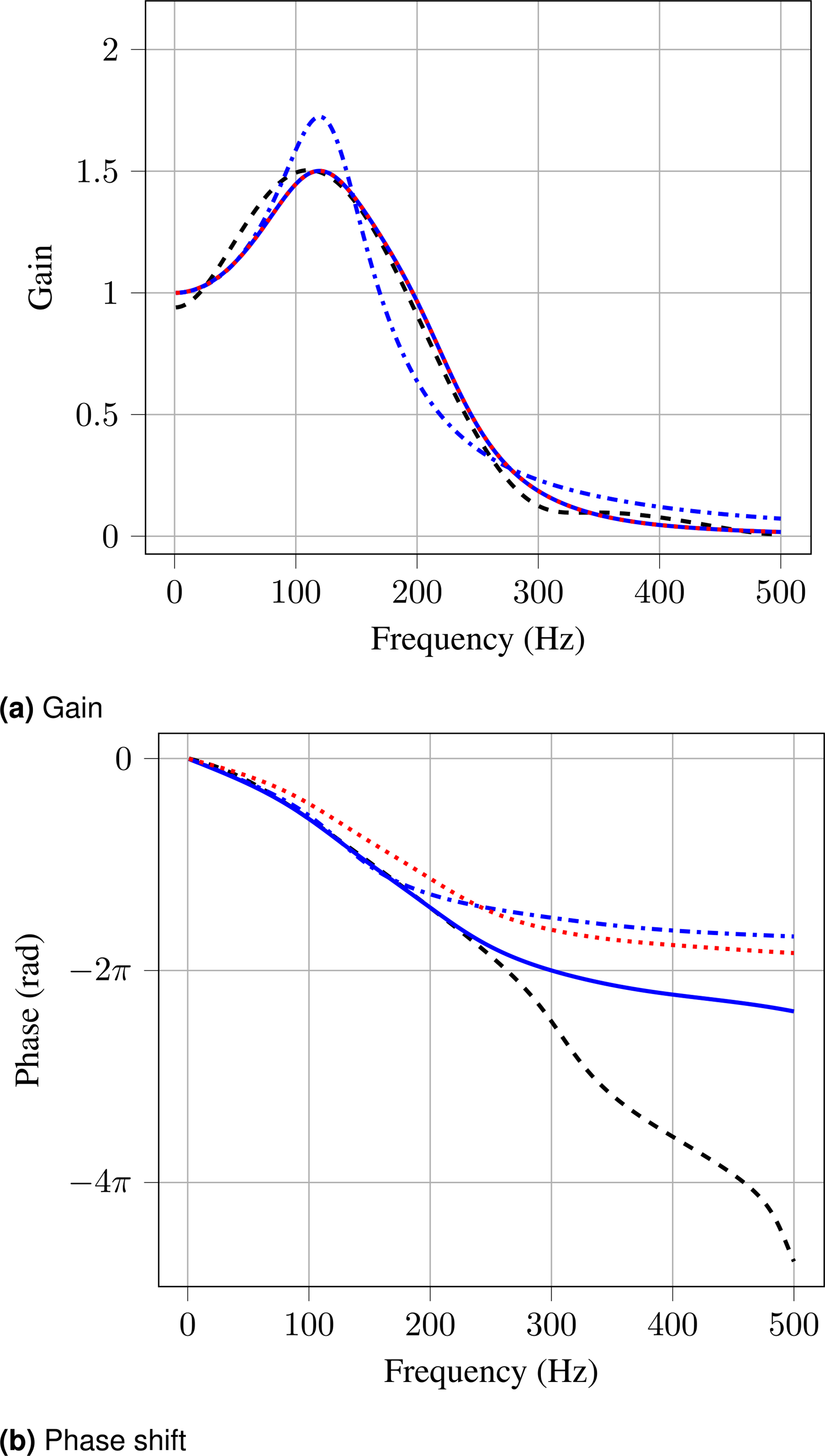
Gain (a) and phase (b) of LDO (blue, solid), LSO (blue, dash dotted) and LDO without delay (red, dotted) after first (linear) stage of optimization.

We start by analysing the impulse response of the obtained LSO and LDO models, both depicted in Figure 5. As pointed out at the beginning of the paper, the impulse response of the flame is remarkably similar to a simple mass-spring-damper system. The LDO is capable of nearly exactly mimicking the impulse response of the flame. Only the initial dip as well as the position and value of the response peak are slightly off-set in comparison to the reference response. The LSO is also capable of modelling large parts of the flame impulse response. Again, the position and magnitude of the peak are off-set from the reference data. In addition, the LSO impulse response separates from the target response around $t = 0.7, : 10^{- 2} s$ and overshoots too strong for larger values. The general trend of model LDO outperforming model LSO significantly is thus also observed in the impulse response.

Next, we analyze the models gain and phase depicted in Figure 6. Up to around $100$ Hz, the LSO gain is smaller than the reference gain, then overshoots significantly and decreases too fast until $280$ Hz. For the rest of the evaluated frequency spectrum the LSO gain remains larger than the reference gain.

To further illustrate the reasoning for a time delay calibration $ς \neq 0$ , we also plot the gain and phase of the optimized LDO with $ς = 0$ after optimization. Similarly to the LSO, the gain of the LDO (with and without time delay) is smaller than the reference gain up to a frequency of around $100$ Hz, but unlike the LSO, both versions of the LDO do not overshoot and match the reference gain nearly perfectly for the rest of the frequency range evaluated. As already pointed out in subsection Manipulating the Phase Response, setting $ς \neq 0$ has no impact on the gain.

Moving on to the phase shift of the LSO and both LDO’s, we can observe that the LSO (which is using a delay) matches the phase characteristics of the flame up to a frequency of around $180$ Hz, whereas the LDO using a delay matches the phase up to approx. $250$ Hz. When comparing the phase of the LDO using a delay with the non-delayed LDO model, we immediately recognize the need for a delayed model architecture. The phase of the non-delayed LDO model cannot match the flame’s phase curve.

Considering the results presented so far, the LDO represents a time domain model capable of modelling the linear dynamics of a laminar premixed flame with satisfactory precision. It does so using only three constants $α$ , $δ$ and $ς$ requiring calibration, whereas the finite impulse response (FIR) model used by Silva et al.¹³ requires calibration of 16 free parameters.

In this work, the LDO represents an intermediate optimization result, which is further extended to also model non-linear aspects of the flame response (namely by parameter $β$ , controlling the non-linear contribution). Note, however, that the here presented intermediate (linear) model can be readily used for linear stability studies.

Results after Non-Linear optimization

So far, the discussed results demonstrate the power of our simple LDO model and its superiority in comparison to the LSO model. We thus refrain from further discussion of the non-linear single mass model (NLSO), although for the sake of completeness its performance on time data is also stated in Table 3.

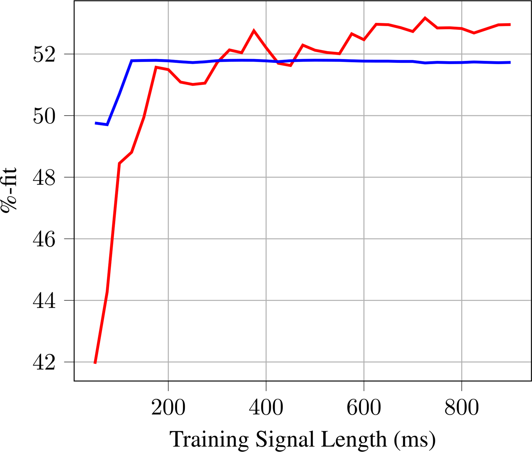
As for the linear models, we analyze the performance in the time domain using a %-fit value. The results are shown in Table 3. When applying the non-linear models to the non-linear data set, compared to the LDO, we can observe an increase of performance in the order of $10 %$ for the NLDO. The accuracy of the presented models on the non-linear data set is far from the excellent performance previously observed on the linear data set, but still very high keeping in mind, that the NLDO comprises of only one additional adjustable constant ( $β$ ). Also note, that there is no drop in performance of the NLDO when applying it to the linear data set. The now active non-linear model contribution does not impair the excellent model performance for linear cases.

Figure 9.

Obtained %-fit by model NLDO on non-linear training data (red curve) and non-linear test data (blue curve) when being optimized on training signals with different lengths.

Figure 7 illustrates the performance of the fully optimized NLDO on linear and non-linear test data. As suggested by the presented %-fit values, performance on the linear data is remarkably good. The basic linear flame dynamics are fully captured by the model at hand. While performance on the non-linear data set is worse, the predictions of the model are still capable of correctly following the dynamics of the flame. Certain features of the flame signal, as well as narrow signal peaks, cannot be fully predicted, but the general, underlying non-linear flame dynamics are very well captured.

Figure 7.

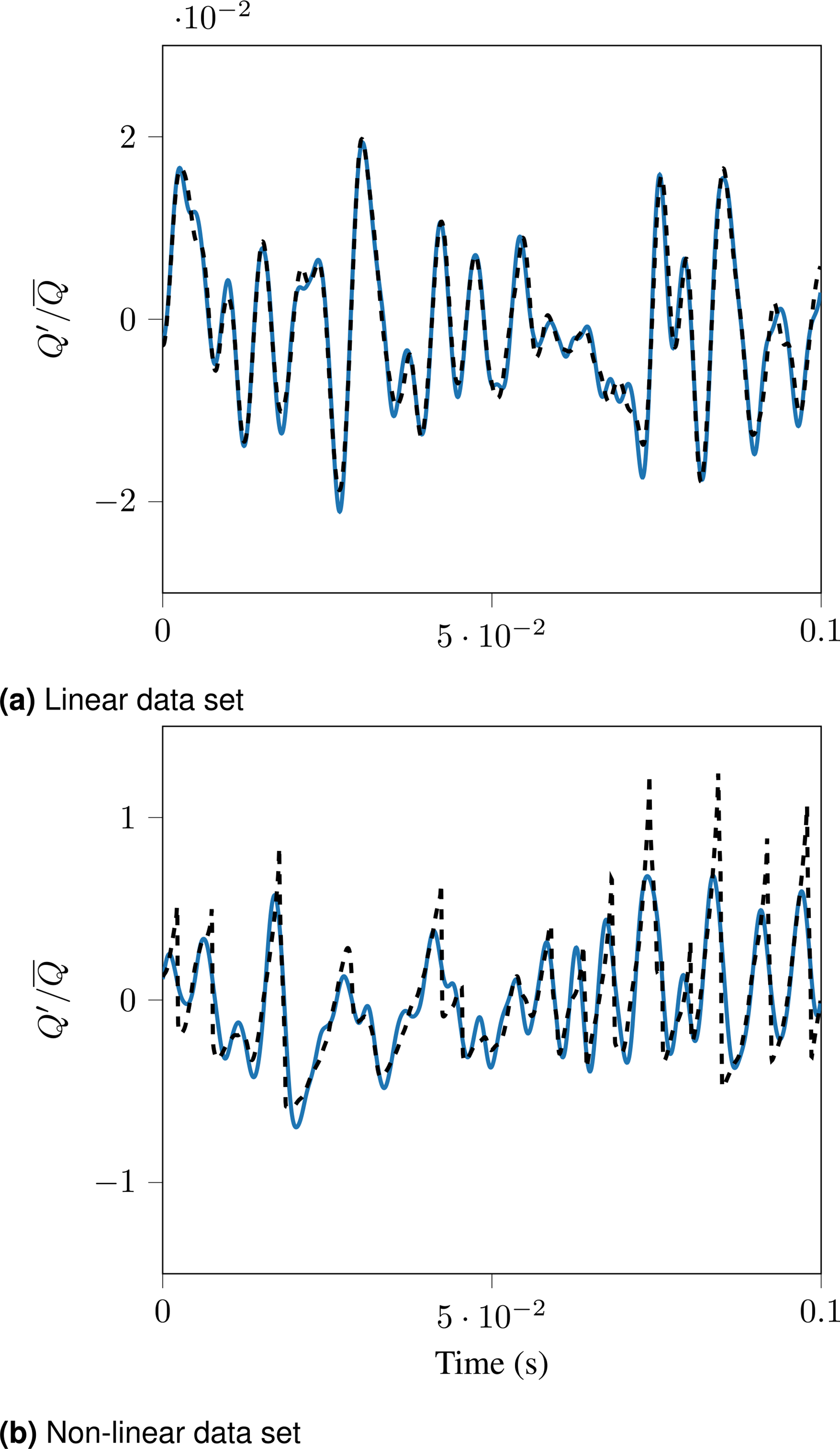
Excerpt comparing the output prediction of the NLDO to reference test data for the linear data set (a) and the non-linear data set (b). Only the last 100 milliseconds are plotted.

As for the linear models, we obtained a model fully characterising the system using only time series data. In post processing, we again assess its frequency response (Figure 8). For the non-linear data case, we use flame frequency response data from Haeringer et al.⁵ as reference data. Starting with the gain, we can observe a good qualitative match of the saturation effects present in premixed flames. The initial slope of the reference gain is matched well for all forcing amplitudes. Gain prediction for the smallest forcing amplitude matches the reference case at best. This excellent match can be explained by our staged optimization approach, which ensures maintaining the good performance for the linear regime demonstrated in Figure 6. The match of gain characteristics decreases with increasing magnitude of the forcing amplitudes - i.e. with further deviation from linear dynamics. Even though, matching of the reference gain characteristics is significantly worse than for the linear case, the physically important low frequency limit of one, the general saturation characteristic as well as the low-pass filter behaviour are well captured. 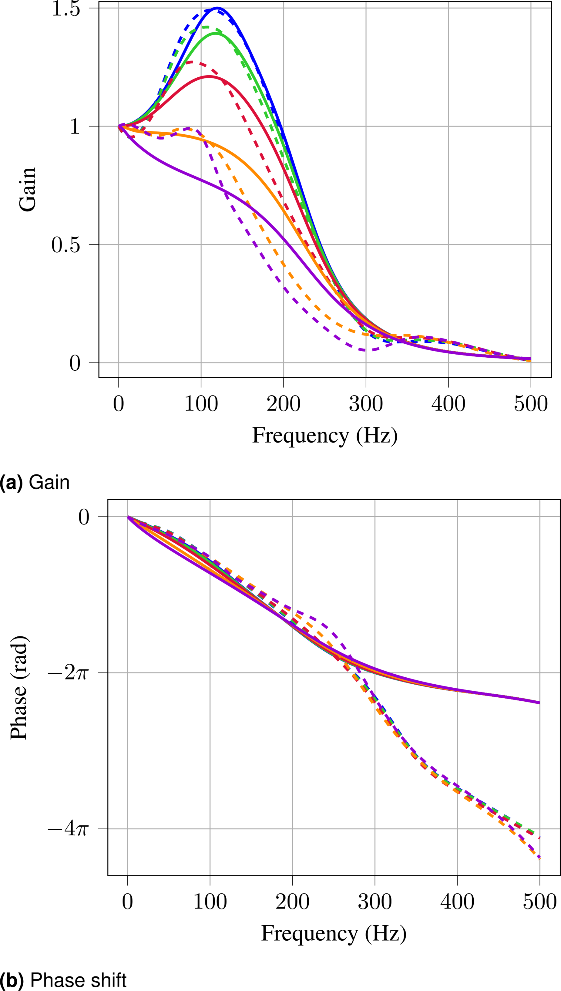Considering the phase prediction of the NLDO model, we observe a good qualitative match for frequencies up to around $280$ Hz. For higher frequencies, we observe an increasing mismatch in phase.

Figure 8.

Gain and phase of the optimized NLDO model (solid) and reference xFDF (dashed). Different colours represent different forcing amplitudes of 0.025 (blue), 0.25 (green), 0.5 (red), 1.0 (orange), 1.5 (purple).

The NLDO model utilizes only four adjustable parameters to achieve the presented effect in the time domain as well as in the frequency domain. The so obtained model is extremely lean in comparison to the reference xFDF model proposed by Haeringer et al.⁵, relying on data from $112$ frequency data points. In addition, we require rather short training signals to achieve the demonstrated performance. As stated in Table 1, the training signal for the linear case is only $\approx 100$ ms long. For the non-linear case, we have to double the length of the signal to $200$ ms to achieve the %-fit performance stated in Table 3. Since the available non-linear training signal is $\approx 900$ ms long, we can investigate how the performance on training and test data behaves when altering the length of the training signal - but not the test signal. The results of this analysis are presented in Figure 9. For training signals longer than $\approx 200$ ms, only the %-fit of the training data increases, while performance on the test data set remains constant. Interestingly, unlike in classic over-fitting cases, the test fit does not decrease with increasing training fit. This demonstrates that the proposed NLDO model is robust and unlikely to suffer from over-fitting. Such a robustness originates from the physical nature of the NLDO itself, i.e. coupled oscillators, which requires only a very small number of parameters for calibration during training. This is a key advantage when comparing the hereby presented model to other more general approaches involving generic filters (system identification of rational functions) or univeral composition of functions (neural networks). The robustness of the NLDO model is especially remarkable when considering the fact that it requires less than $25 %$ of the original training signal length Jaensch and Polifke¹⁹ used to train their neural network.

Conclusions and outlook

In this work we have shown that two mass-spring-damper coupled oscillators with only one non-linear term in its two equations – a remarkable simplification of Eq. (2) – is sufficient for a good qualitative representation of the non-linear flame response of a typical laminar premixed flame. Following an optimization approach that makes use of time series data stemming from CFD, the four parameters of the model are calibrated. No a-priori knowledge of the FTF or FDF of the system under investigation is required. The soundness of the proposed phenomenological model becomes evident when evaluating not only the impulse response and corresponding frequency response (FTF) but also the describing function (FDF) of the trained model. We show that the model labelled as NLDO is able to capture the low-pass filter behaviour, the low frequency limit and the gain saturation that a typical FDF exhibits. To our knowledge, no other ODE model exists that is capable of retrieving the aforementioned three characteristics. A Wiener-Hammerstein model (see Dowling³ for example) would not be able to capture the low frequency limit as it assumes a static saturation related to the input or output.

Equation (2) and the results presented may suggest that better results could be obtained if additional dimensions (additional oscillators) are considered in the model. Indeed, the increase in performance when adding one additional mass (switching from LSO to LDO) is evident not only from the %-fit values stated in table 3 but can also be observed in the impulse response (Figure 5), as well as in gain and phase (Figure 6). This increase in performance can largely be attributed to an improved phase modelling. Thus, adding more oscillators to the system could be of help if the phase description accuracy given by the model needs to be increased. Note, however, that a further increase in the number of masses, and thus oscillators significantly increases the complexity of the model, which may be detrimental for the optimization procedure.

When deriving the model Eqs. (18) and (19) describing the NLDO, we assumed a uniform parametrization of the masses. This assumption reduces the number of adjustable parameters significantly. One could assume a non-uniform parametrization in the described method, also obtaining well performing models. The performance, however does not improve significantly, while the complexity of the model does.

In the presented work we limited the addition of non-linear terms to one term $x^{2} \dot{x}$ , keeping the overall model rather simple. Results presented in Figure 8 demonstrate that this term is essential for capturing general saturation dynamics but not sufficient on its own. Future work could investigate the possibility to extend the capacities of the non-linear model by either adding more non-linear terms that have not been investigated in depth yet or creating a new model of hybrid type. In such a case, the linear system could be characterized by a system of coupled, linear oscillators (such as the LDO proposed in this work), whereas the non-linear terms may be described by generic, composite functions, as the ones used in classical neural network architectures. As a matter of fact, further work in this direction can be leveraged by novel machine learning techniques such as neural ODEs Chen et al.²⁴ or sparse identification of nonlinear dynamics Brunton and Kutz²⁵.

An additional extension of the present work could focus on data coming from turbulent premixed flames. At that point it would be interesting to evaluate the robustness of the coupled oscillator model when presented to data corrupted by noise, which in that case is directly related to the noise produced by combustion. It is also of high interest to determine how many additional dimensions are required in order to retrieve features typical of turbulent flames, such as crests and valleys (local maxima and minima) in the gain response. A practical way of increasing the amount of dimensions – and thereby the power capability of the model – may consist of a mere linear superposition of NLDOs. Such a strategy is currently being investigated in our group.

The non-linear flame response model proposed is a parsimonious set of ODEs. Accordingly, it is a continuous-time model and, as such, is ideal for inexpensive, time-domain acoustic simulations (when coupled with appropriate low-order acoustic models), where signals exhibit a broad amplitude and frequency distribution. Note that, contrary to time-domain low-order models coupled with an FDF, no knowledge of the instantaneous amplitude and frequency of the signals is required.

Footnotes

Acknowledgements

The authors gratefully acknowledge the Research Association for Combustion Engines (Forschungsvereinigung Verbrennungskraftmaschinen e.V. FVV, project number 6012700) for the financial support to Matthias Haeringer and the compute and data resources provided by the Leibniz Supercomputing Centre ().

Data and Code Availability

The code used for optimization and post processing as well as all data used in this work is available at

ORCID iDs

Gregor Doehner

Matthias Haeringer

References

Lieuwen

Yang

(eds.) Combustion Instabilities in Gas Turbine Engines: Operational Experience, Fundamental Mechanisms and Modeling. Number v. 210 in Progress in Astronautics and Aeronautics. Reston, VA: American Institute of Aeronautics and Astronautics, 2005. ISBN 978-1-56347-669-3.

Poinsot

. Prediction and Control of Combustion Instabilities in Real Engines. Proc Combus Inst 2017; 36: 1–28. DOI: 10.1016/j.proci.2016.05.007.

Dowling

. Nonlinear Self-excited Oscillations of a Ducted Flame. J Fluid Mech 1997; 346: 271–290. DOI: 10.1017/S0022112097006484.

Noiray

Durox

Schuller

Candel

. A Unified Framework for Nonlinear Combustion Instability Analysis Based on the Flame Describing Function. J Fluid Mech 2008; 615: 139–167. DOI: 10.1017/S0022112008003613.

Haeringer

Merk

Polifke

. Inclusion of Higher Harmonics in the Flame Describing Function for Predicting Limit Cycles of Self-excited Combustion Instabilitites. Proc Combus Inst 2018; 37(4): 5255–5262. DOI: 10.1016/j.proci.2018.06.150.

Ghirardo

Ćosić

Juniper

Moeck

. State-space Realization of a Describing Function. Nonlinear Dyn 2015; 82(1-2): 9–28. DOI: 10.1007/s11071-015-2134-x.

Tathawadekar

Doan

Silva

Thuerey

. Modelling of the nonlinear flame response of a Bunsen-type flame via multi-layer perceptron. 38th Symposium on Combustion, 2021. DOI:10.1016/j.proci.2020.07.115.

Campa

Juniper

. Obtaining bifurcation diagrams with a thermoacoustic network model. In: ASME Turbo Expo 2012: Turbine Technical Conference and Exposition. American Society of Mechanical Engineers, 2012, pp.167–177.

Noiray

Schuermans

. On the Dynamic Nature of Azimuthal Thermoacoustic Modes in Annular Gas Turbine Combustion Chambers. Proceedings of the Royal Society A: Mathematical, Physical and Engineering Sciences 2013; 469(2151): 20120535. DOI: 10.1098/rspa.2012.0535.

10.

Noiray

. Linear Growth Rate Estimation From Dynamics and Statistics of Acoustic Signal Envelope in Turbulent Combustors. J Eng Gas Turbine Power 2017; 139(4): 041503. DOI: 10.1115/1.4034601.

11.

Bonciolini

Faure-Beaulieu

Bourquard

Noiray

. Low Order Modelling of Thermoacoustic Instabilities and Intermittency: Flame Response Delay and Nonlinearity. Combust Flame 2021; 226: 396–411. DOI: 10.1016/j.combustflame.2020.12.034.

12.

Gant

Ghirardo

Bothien

. On the Importance of Time Delay and Noise in Thermoacoustic Modeling. J Sound Vib 2021; 501: 116067. DOI: 10.1016/j.jsv.2021.116067.

13.

Silva

Emmert

Jaensch

Polifke

. Numerical Study on Intrinsic Thermoacoustic Instability of a Laminar Premixed Flame. Combust Flame 2015; 162(9): 3370–3378. DOI: 10.1016/j.combustflame.2015.06.003.

14.

Lieuwen

. Statistical Characteristics of Pressure Oscillations in a Premixed Combustor. J Sound Vib 2003; 260(1): 3–17. DOI: 10.1016/S0022-460X(02)00895-7.

15.

Noiray

Schuermans

. Deterministic Quantities Characterizing Noise Driven Hopf Bifurcations in Gas Turbine Combustors. Int J Non Linear Mech 2013; 50: 152–163.

16.

Polifke

Lawn

. On the Low-Frequency Limit of Flame Transfer Functions. Combust Flame 2007; 151(3): 437–451. DOI: 10.1016/j.combustflame.2007.07.005.

17.

Lunze

. Regelungstechnik. 1: Systemtheoretische Grundlagen, Analyse und Entwurf einschleifiger Regelungen: mit 64 Beispielen, 166 Übungsaufgaben sowie einer Einführung in das Programmsystem MATLAB. Springer-Lehrbuch, 5., neu bearb. und erw. aufl edition. Berlin: Springer, 2006. ISBN 978-3-540-28326-3.

18.

Kornilov

Rook

ten Thije Boonkkamp

JHM

de Goey

LPH

. Experimental and Numerical Investigation of the Acoustic Response of Multi-Slit Bunsen Burners. Combust Flame 2009; 156(10): 1957–1970. DOI: 10.1016/j.combustflame.2009.07.017.

19.

Jaensch

Polifke

. Uncertainty Encountered When Modelling Self-Excited Thermoacoustic Oscillations with Artificial Neural Networks. Int J Spray Combust Dyn 2017; 9(4): 367–379. DOI: 10.1177/1756827716687583.

20.

Strogatz

. Nonlinear Dynamics and Chaos: With Applications to Physics, Biology, Chemistry, and Engineering. Studies in Nonlinearity, 2. print edition. Cambridge, Mass: Perseus Books, 2001. ISBN 978-0-7382-0453-6.

21.

Blumenthal

Subramanian

Sujith

Polifke

. Novel Perspectives on the Dynamics of Premixed Flames. Combust Flame 2013; 160(7): 1215–1224. DOI: 10.1016/j.combustflame.2013.02.005.

22.

Steinbacher

. Analysis and Low-Order Modeling of Interactions between Acoustics, Hydrodynamics and Premixed Flames. PhD Thesis, TU München, München, 2019.

23.

Byrd

Nocedal

Zhu

. A Limited Memory Algorithm for Bound Constrained Optimization. SIAM J Sci Comput 1995; 16(5): 1190–1208. DOI: 10.1137/0916069.

24.

Chen

Rubanova

Bettencourt

Duvenaud

. Neural Ordinary Differential Equations : 13, 2018.

25.

Brunton

Kutz

. Data-Driven Science and Engineering: Machine Learning, Dynamical Systems, and Control. Cambridge: Cambridge University Press, 2019.

Nonlinear flame response modelling by a parsimonious set of ordinary differential equations

Abstract

Keywords

Introduction

Model description

Mathematical motivation

Physical motivation

General model equations

Non-linear contributions

Low-frequency limit

Manipulating the phase response

Method

Input and target data

Time scaling of the equations

Optimization

Results and analysis

Results after linear optimization

Results after Non-Linear optimization

Conclusions and outlook

Footnotes

Acknowledgements

Data and Code Availability

ORCID iDs

References