Sage Journals: Discover world-class research

Abstract

Much discussion surrounds the flight of association footballs (soccer balls), particularly where the flight may be perceived as irregular. This is particularly prevalent in high-profile competitions due to increased camera coverage and public scrutiny. All footballs do not perform in an identical manner in flight. This article develops methods to characterise the important features of flight, enabling direct, quantitative comparisons between ball designs. The system used to generate the flight paths included collection of aerodynamic force coefficient data in a wind tunnel, which were input into a flight model across a wide range of realistic conditions. Parameters were derived from these trajectories to characterise the in-flight deviations across the range of flights from which the aerodynamic performance of different balls were statistically compared. The amount of lateral movement in flight was determined by calculating the final lateral deviation from the initial shot vector. To quantify the overall shape of the flight, increasing orders of polynomial functions were fitted to the flight path until a good fit was obtained with a high-order polynomial indicating a less consistent flight. The number of inflection points in each flight was also recorded to further define the flight path. The orientation dependency of a ball was assessed by comparing the true shot to a second flight path without considering orientation-dependent forces. The difference between these flights isolated the effect of orientation-dependent aerodynamic forces. The article provides the means of quantitatively describing a ball’s aerodynamic behaviour in a defined and robust mathematical process. Conclusions were not drawn regarding which balls are good and bad; these are subjective terms and can only be analysed through comprehensive player perception studies.

Keywords

Football soccer ball aerodynamics ball performance flight characterisation orientation sensitivity

Introduction

Association football (soccer) is the most viewed and played sport in the world. Having a satisfactory ball design is of great importance, particularly in high-profile competitions. All footballs do not perform in an identical manner; for example, Passmore et al.¹ measured considerable variation in aerodynamic loads for a range of Fédération Internationale de Football Association (FIFA)-approved footballs that will lead to differences between flight paths. While standards exist for controlling the performance of footballs with regards to circumference, sphericity, rebound, water absorption, weight, and pressure loss,² standards do not exist for the flight, nor are there accepted methods to quantify or characterise aerodynamic performance. The ability to develop these methods would be fundamental in the creation of effective standards in this area, as well as being advantageous for prototype development.

This article defines methods to describe or characterise the flight of a ball. The methodology used to generate flights is to measure aerodynamic force coefficients for a given ball against a range of airspeeds, spin speeds, and orientations using wind tunnel techniques developed by Passmore et al.³ The measured data are then used in a flight model to generate simulated trajectories for a range of realistic input conditions. From this data, characterisation parameters are derived to describe the ball’s overall in-flight behaviour. Analysing these parameters across a prescribed set of flights can measure a ball’s performance or directly compare the characteristics of many balls. The objective of this article was to describe and evaluate methods of quantifying performance, not to determine which balls are good or bad. Subjective player tests that are likely to show differences in opinion, for example, between strikers and goalkeepers, would address the perceived performance of a ball.

Background

The huge rise in the popularity of sport in the last half century and intense observation of its every aspect have introduced a need to understand the science behind sporting equipment, including the aerodynamics of balls. Analysis of the aerodynamics of smooth and rough spheres was completed by Achenbach^4,5 and is widely used for comparison against various sports balls. Achenbach identified four key regions of flow around a sphere: sub-critical, critical, supercritical, and trans-critical. Achenbach presented data on the flow separation in each of these regimes that can be used to explain the flow’s behaviour and measured aerodynamic loading on the sphere. Achenbach⁴ showed that by adding roughness to the sphere surface, one can control the critical Reynolds number $(R e_{crit})$ , and hence, the aerodynamic behaviour of the ball in the expected range of airspeeds.

Significant works have applied these fundamentals to sports balls, particularly to golf balls, cricket balls, and baseballs. Mehta’s review⁶ of these balls collates pressure and force data, as well as visualisation of how the ball’s features can be used to control the flow around the ball. For example, a cricket ball’s seam introduces different separation locations, hence causing a lateral force, colloquially known as swing. Passmore et al.^1,3 present a comprehensive, wind-tunnel-based analysis of the aerodynamics of footballs and how the features of the ball can affect the measured aerodynamic forces and a prediction of how this can alter the flight path a ball might take. Their article includes a summary of much of the existing work in the field and thus is not repeated here.

Use of a wind tunnel to measure the aerodynamic loads has the advantage that the drag, lift, and lateral contributions can be separated and their effects examined independently or combined within a flight model. As shown in previous studies, lateral forces in flight arise from spinning the ball, as well as asymmetry in seam geometry and orientation.^1,3,6–8

Asymmetric seam positions can introduce highly unpredictable deviations in flight, particularly at low spin speeds. Passmore et al.⁷ measured forces against yaw angle for a range of spin rates and Reynolds number (Re), a set of which at 25 m/s (Re = 3.6 × 10⁵) can be seen in Figure 1(a). The mean side force (i.e. Magnus force) can be seen to increase with spin rate with the orientation-dependent forces still evident, although smaller than in the static case. At a sub-critical speed of 10 m/s (Re = 1.4 × 10⁵), the magnitude of the forces are smaller and the effect of orientation quickly diminishes with increasing spin rate, as shown in Figure 1(b). Different behaviours are exhibited at different speeds and spin rates, making the prediction and modelling of such flights more complex. While the flights produced from low spin shots are predictable from aerodynamic data, they are unlikely to be within the control of players to execute consistently and impossible for a goalkeeper to predict. Similar conclusions were drawn by Barber et al.⁹

Figure 1.

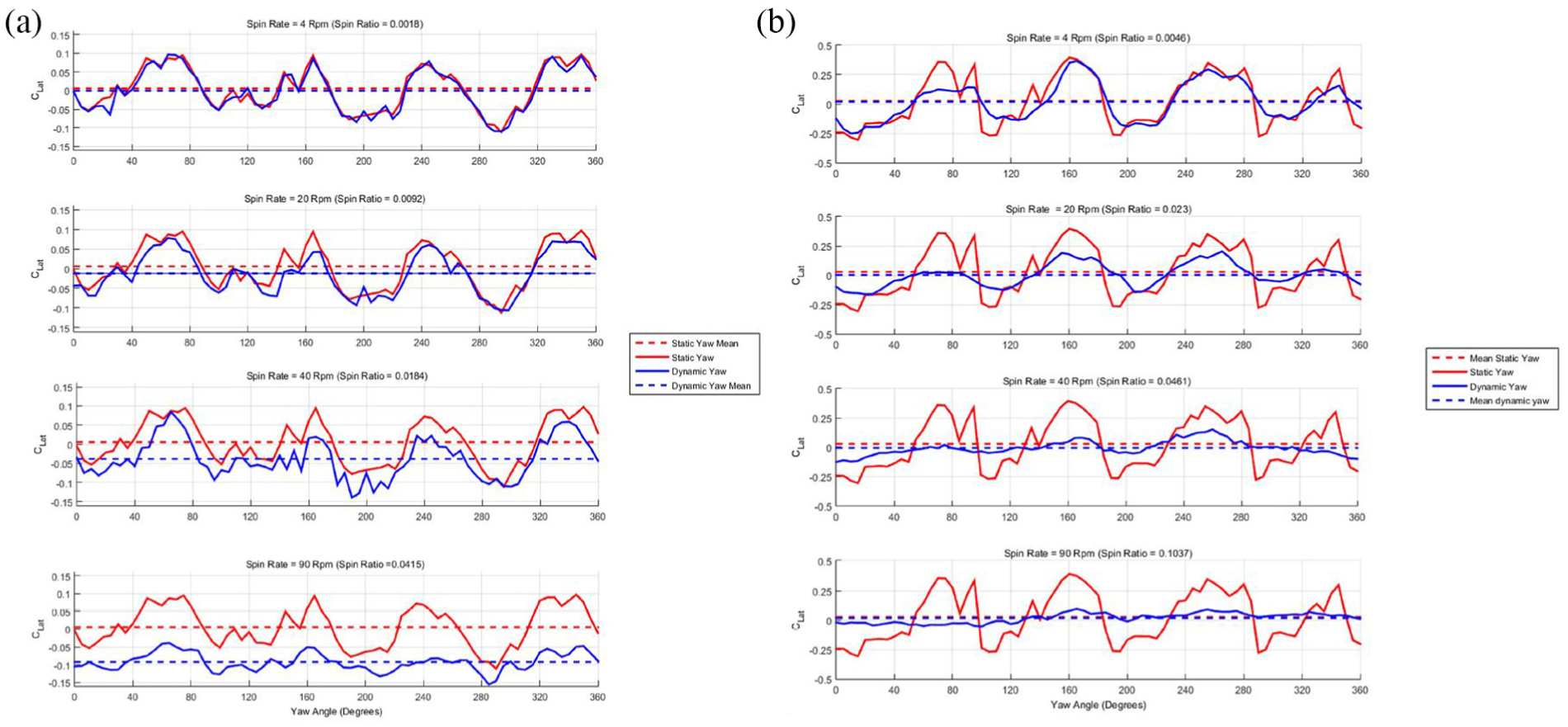
Lateral coefficients against orientation – brazuca spinning ball: (a) 25 m/s and (b) 10 m/s.⁷

The lateral forces introduced by spin are generally predictable due to the Magnus effect, although combined low spin speeds and Re can lead to reverse Magnus forces. A simplified sketch (Figure 2) shows these effects; more detail can be found in Kim et al.¹⁰ The Magnus force operates by reducing the velocity difference between flow and surface on the upper side, allowing the flow to stay attached longer on that side, with the opposite effect occurring on the lower side, resulting in a net upwards force. 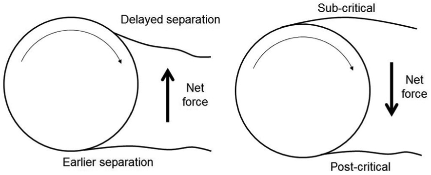The reverse Magnus effect occurs around $R e_{crit}$ , where the flow on the upper side becomes sub-critical, moving the separation location significantly upstream; the lower side remains post-critical, meaning its separation location is further downstream, resulting in a net downwards force.

Figure 2.

Sketch indicating the mechanics behind (left) conventional and (right) reverse Magnus effects.

Football manufacturers typically assess football flight characteristics using kicking tests conducted by players. These tests can produce some insight into the ball’s aerodynamic behaviour, but the tests are subjective, usually have low sample size and are subject to test conditions, player fatigue, and poor repeatability. Some improvement in consistency is possible through the application of a mechanical kicking robot, where the flight is recorded for further analysis; although even with such a mechanical test, difficulties exist in effectively recreating initial conditions.¹¹ This inconsistency results in significant variation in the flight trajectories and the need to establish a high number of repeat kicks to ensure an appropriate sample size for thorough statistical analysis. For recording the ball flight, radar tracking systems¹¹ and high-speed video systems^8,12 tend to be difficult to initially set up, slow to repeat, and none have been proven to be sufficiently accurate for detailed flight assessment, such as orientation effects.¹³ To develop a high-fidelity flight model and subsequent post-processing techniques to directly compare the flight characteristics of balls from wind tunnel data will reduce the need to physically test the aerodynamics of new prototype balls in such an uncontrolled way.

Characterisation procedure

Most papers in the field of football aerodynamics measure the forces on a range of balls and then run a selection of shots through a flight model, similar to the one described in this article, to demonstrate the difference between balls. However, the extracted data are rarely in the same format, which can make further comparisons difficult. Passmore et al.³ show a ‘top down’ view comparing lateral movement. Asai and Seo¹⁴ show the effect of drag by plotting the ball path in the vertical plane. Murakami et al.¹⁵ show the lateral deviation against time, and Hong et al.¹⁶ show the difference in point of impact. While all of these methods are applicable and useful to the study in question, not having standardised tests or performance measures makes it impossible to compare results between the tests.

To begin to quantify the characteristics of different balls in a more standardised way, a technique was developed by Rogers et al.¹¹ to analyse the root mean square (RMS) lateral deviation relative to an initial shot vector for simulated and real recorded trajectories. Rogers¹⁷ also introduced methods such as counting the number of major and minor inflections and calculating an auto-correlation value to describe the predictability of the flight path. These methods are discussed and analysed with other alternatives later in this article.

This article develops and uses a procedure that will enable a ball manufacturer to obtain information about their ball’s aerodynamic characteristics and directly compare them to other balls that have undertaken the same tests. The procedure starts with testing the ball in question to obtain aerodynamic drag and side force measurements. While this article used a wind tunnel and force balance to obtain these data, alternative experimental methods or computational models could also be used. These forces were then used in a flight model to generate a range of trajectories with a range of input conditions, such as launch speed or spin speed. These flights were statistically analysed to obtain a picture of the ball’s aerodynamic performance. Each of these steps is explained in more detail in this article.

Experimental method

A low-speed, open-circuit, closed-jet wind tunnel with a 1.32 m × 1.92 m working section was used for the experimental work in this article. The tunnel is capable of achieving a maximum velocity of 45 m/s and an upper Re of 7 × 10⁵ in the working section based on a football diameter of 0.22 m. In this tunnel, a size 5 football or similar prototype produces a blockage ratio of approximately 1.70%. Thus, the subsequent results have not been corrected for blockage. The clean tunnel turbulence intensity was measured in accordance with Johl et al.¹⁸ using a constant-temperature hot-wire anemometer, as 0.15% at 40 m/s. The boundary layer thickness $(δ^{99})$ at the model position was 60 mm and displacement thickness $(δ)$ of 7.5 mm (at 40 m/s). Further details of the design and performance of the tunnel can be found in Johl et al.¹⁸

The ball was mounted from below in the tunnel as seen in Figure 3(a). A 20 mm silver steel shaft was selected, as this does not deflect significantly under loading (0.47 mm at 10 N at 0.6 m) while also being less than the recommended 10% of the ball diameter.⁵ A clearance of one ball diameter from the tunnel floor was chosen to avoid boundary layer interference and streamline compression.¹⁸ The aerodynamic balance is a high-accuracy, six-axis under-floor, virtual centre balance designed for aeronautical and automotive testing (Figure 3(b)). The quoted accuracy for the relevant balance components is ±0.012 N for drag and ±0.021 N for side force. Using an estimate of the expected forces from a football, the resolution is approximately ±0.05% and ±0.50% full scale for the drag and lateral components, respectively. Details of the spin motor can be found in Passmore et al.⁷

Figure 3.

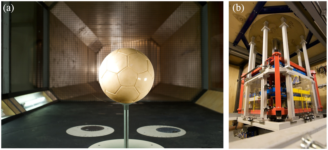
(a) Ball in wind tunnel and (b) six-axis virtual centre balance.

Time-averaged force measurements taken over a 120-s period were converted into the non-dimensional drag and lateral coefficients using equation (1)

C_{D} = F_{D} / (\frac{1}{2} ρ A V^{2}) C_{Y} = F_{Y} / (\frac{1}{2} ρ A V^{2})

(1)

where $F, ρ, A$ , and $V$ are the force, air density, ball frontal area, and relative velocity, respectively.

Reynolds sweeps were undertaken on the test balls in 5 m/s steps from 5 to 35 m/s with 1 m/s steps used from 10 to 20 m/s through the transition regime. The spin tests consisted of Reynolds sweeps at a range of spin rates. The support interference effect was measured and subtracted to obtain an estimate of the true ball forces (see Passmore et al.⁷). Frame of reference corrections were made for the drag and lateral components as the balance rotated. The calculated coefficients used the projected frontal area of the ball as the reference area, calculated from the measured mean ball diameter.

Wind tunnel measurements

Three FIFA-approved balls with different numbers of panels and surface textures were selected for sample testing using the methodology described by Passmore et al.^1,3,7. These data are provided as an example of what is required for robust flight prediction for spinning balls with orientation dependency. A 32-panel prototype ball can be seen in Figure 3(a). 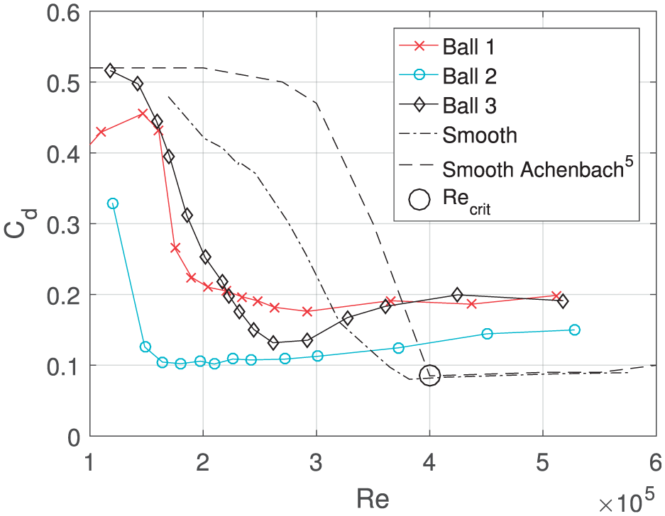Although this article is primarily focused on the lateral forces, the results for drag coefficient $(C_{d})$ against Re are presented in Figure 4. For comparison, a smooth sphere tested using this method and Achenbach’s results⁵ are also included in Figure 4. These tests were run using a rear mounted support to be consistent with Achenbach, although a magnetically supported sphere was tested by Sawada and Suda.¹⁹ The effects of mounting from the rear or from below are discussed by Passmore et al.¹ and not revisited here.

Figure 4.

Reynolds number (Re) sensitivity of balls compared to smooth sphere.⁵

These balls show a broadly similar overall drag profile, but with subtle differences in drag coefficient through transition and in the post-critical region. It can be seen that Ball 3 has the lowest post-critical drag and Ball 2 has the lowest $R e_{crit}$ . For reference, the $R e_{crit}$ (minimum drag value⁵) of Achenbach’s data is circled. A transition point of $Re = 2 \times 1 0^{5}$ equates to a velocity of approximately 13 m/s, at which point the ball is not in the air long enough for the aerodynamics to have a significant effect when compared to realistic kicks. Even large differences in the drag characteristic have a limited effect on the flight, changing the total flight time and end velocity by only a small amount of less than 5%.¹

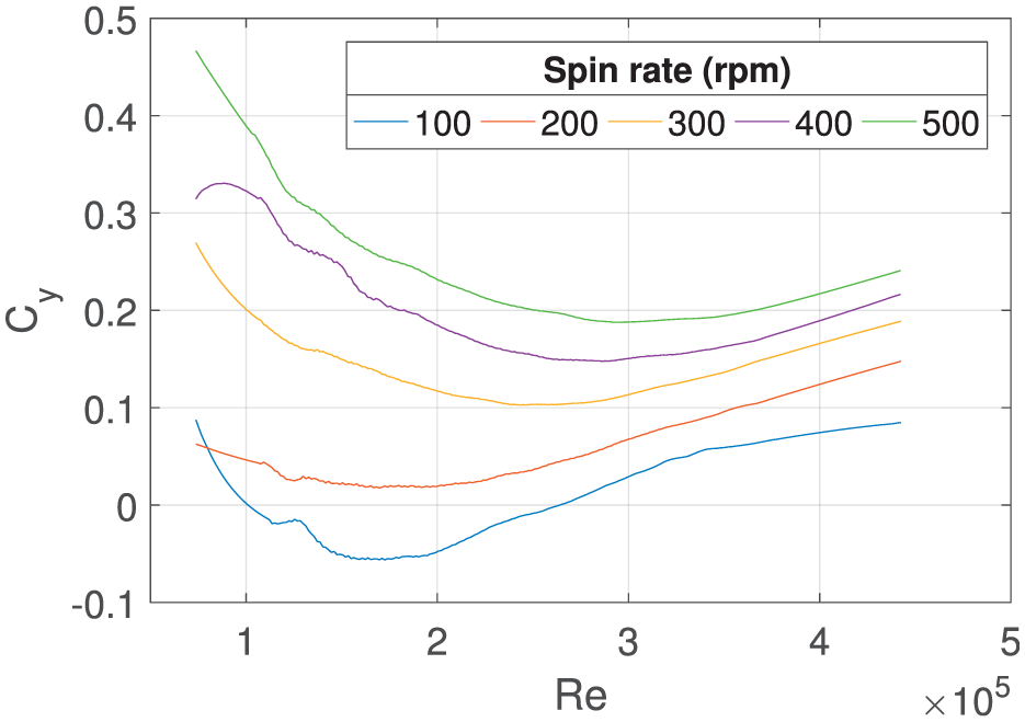
As previously discussed, lateral forces can arise due to spin or asymmetric seam arrangements. The lateral force coefficient $(C_{y})$ for a single ball at a range of spin rates against Re can be seen in Figure 5. As expected, the force increases with both Re and spin rate, with an exception at low values where a reverse Magnus effect can be seen.

Figure 5.

Effect of spin rate (in rpm) on lateral force coefficient.

The change in forces with orientation is dependent on both the spin rate and airspeed. To collect data at low spin speeds (where this behaviour is most significant), the method defined in Passmore et al.⁷ was used. A sample set of data is shown in Figure 1.

Flight model

A large number of shots are required for effective overall characterisation due to (1) the need to capture the full range of possible flight conditions and (2) the statistically based methods used in post-processing. Despite the volume of runs to be undertaken, a good degree of accuracy must be maintained for any meaningful conclusions to be drawn. A flight model is an ideal tool to undertake these tasks; its Newtonian physics are simple to compute and unlikely to introduce significant further errors into the prediction. The flight model developed follows similar principles to those reported by Bray and Kerwin¹², Myers and Mitchell,²⁰ and Tuplin et al.²¹ At each time step, an interpolation of the wind tunnel data for the particular ball type at the current Re, spin rate, and orientation was performed to obtain the drag, lift, and lateral force coefficients. It should be noted that these values could also be obtained using other methods such as computational fluid dynamics (CFD) modelling or calculation from recorded trajectories,²² although these have not yet been proven to be as effective or controllable as wind tunnel testing. These values were converted into accelerations and integrated across the time step to calculate new velocity and position values, which were then used as inputs for the next time step. This flight model can be used to predict a large number of kicks across a representative range of initial launch conditions that can then be statistically analysed to characterise the overall performance of the ball. This is described mathematically in equations (2)–(5)

F_{x} = F_{D_{x}} + F_{M_{x}} + F_{O_{x}} + F_{g_{x}}

(2)

{\overset{\cdot\cdot}{x}}_{n} = F_{x} / m

(3)

{\overset{\cdot}{x}}_{n + 1} = {\overset{\cdot\cdot}{x}}_{n} * dt

(4)

x_{n + 1} = {\overset{\cdot}{x}}_{n + 1} * dt

(5)

where $F_{D_{x}}, F_{M_{x}}, F_{O_{x}}$ , and $F_{g_{x}}$ are the components of the drag, Magnus (spin-dependent), orientation-dependent, and gravitational forces acting in the $X$ direction, respectively. Similar processes are carried out for $Y$ , $Z$ , and spin axes. For further information, see Tuplin et al.²¹

For consistency and clarity in the tests, the spin axis was assumed to be vertical (and through the valve of the ball), although other spin axes are possible (e.g. a goal kick may be struck with almost entirely backspin). Using this assumption allows the lateral effects to be analysed in isolation from gravitational forces. One could use a horizontal spin axis and analyse the longitudinal against vertical trajectory in the same way this article studies the longitudinal against lateral movement. However, the spin and orientation-dependent forces would be the same, but obscured by gravitational forces and more difficult to examine. The gravitational force cannot simply be removed, as it changes the vertical velocity component in flight, which will change the aerodynamic forces experienced by the ball. This was demonstrated by Myers and Mitchell.²⁰

The simulation is assumed to begin after the ball has regained its shape after contact, which was quantified by Shinkai et al.²³ to last in the order of 10 ms (equating to around 1 diameter of travel). The optimum time step was determined using first-order backward differencing, where the time step has been reduced until there is no significant change in the calculated flight path.

Input parameters

For accurate comparisons between different balls, a standardised set of input parameters must be defined. The initial parameters are: velocity $(V)$ , spin rate $(ω)$ , velocity elevation angle $(α)$ , and initial yaw orientation of the ball $(ψ)$ . The velocity azimuthal angle remains constant at zero, and it is assumed the valve of the ball is at the bottom pole. Environmental constants such as air density, viscosity, and gravitational acceleration should be assumed to be as at sea level, unless otherwise stated (e.g. investigating effects of altitude). Wind speeds are also assumed to be zero and the spin axis of the ball assumed to be vertical (see the ‘Flight model’ section for justification). All combinations of $V$ , $ω$ , $α$ , and $ψ$ are studied, totalling 7280 flights per ball. The range of values is shown in Table 1. Notation of $x : y : z$ indicates ‘from $x$ to $z$ in intervals of $y$ ’.

Table 1.

Range of test input parameters.

Variable	Values	Unit	Count
V	10:5:30	m/s	5
$ω$	0:2.5:15, 20:5:45, 50:25:400	rpm	28
$α$	10:10:40	°	4
$ψ$	–150:30:180	°	13

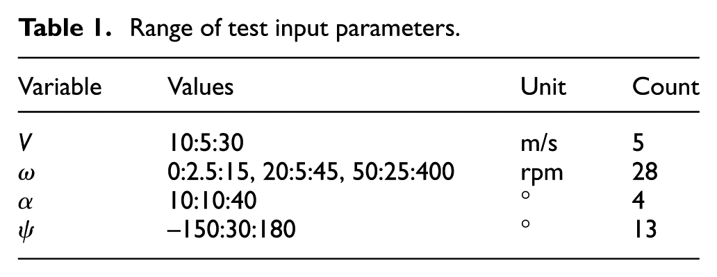
These values aim to test a representative range of shots. Velocities below 10 m/s are not in the air long enough for aerodynamic forces to have a significant effect. The maximum speed is limited by the sensitive spin balance that can be overloaded at very high spin rates and airspeeds. The chosen spin speeds are aimed to test low spin rates where orientation-dependent forces dominate,⁷ high spin where Magnus forces dominate and some intermediate points where both are significant. The elevations primarily aim to incorporate the effect a longer duration may have on the flight, but there is also an element of understanding the effect of changing the velocity in flight. A steeper launch will have a greater vertical velocity component, which will become zero at the apex of the shot. The reduction this has on the velocity magnitude can introduce phenomena such as the reverse Magnus effect, which would not be seen at lower elevations. Finally, the yaw positions are intended to test the sensitivity of the ball to the start orientation.

While there is no definitive dataset on football shot speeds and spin rates publicly available, it is believed that Table 1 gives a balanced overall measure of the ball’s characteristics, based on literature in the field and anecdotal evidence. A more definitive dataset will be an important addition to develop test protocols and standards in the future. Specific aspects of a ball’s performance can be assessed by deliberately manipulating the input parameters. For example, if a ball’s low spin performance was of particular interest, using more, or only, low spin rates can bias the results. All four of the parameters can affect the final results, so it is important that they reflect the analysis required.

Flight characterisation techniques

It is the aim of this article to develop standardised methods of drawing direct, quantitative comparisons between ball designs to improve performance analyses. In this article, a ball’s performance is characterised by quantifying the amount of lateral movement in the air, including the shape of a ball’s flight and how orientation-dependent the lateral forces are on the ball. When these characteristics are combined across a pre-determined range of flights, an overall performance profile can be built for the ball under test. The key elements of a good measure of performance are that it can be statistically combined across a range of shots, is simple to interpret into real terms, and is sensitive enough to differentiate between balls. This section presents a number of potential measures and outlines the positives and negatives of each.

Central tendency measures

The first approach to characterising a ball’s performance is to quantify the deviation from a central tendency, such as the initial shot vector or from a line drawn from the start to finish points. Two methods to do this are the end and maximum lateral deviations (ELD and MLD) from the initial shot vector. Another potential measure is the RMS residual deviation, referred to as residual. This is defined as the RMS of the distances for each point of the flight path from a line drawn between the initial and final positions. This value is then the average deviation from a straight flight. A graphical description of these methods and the results for these flights can be seen in Figure 6. The ELD describes how far the ball finished from the initial shot vector. If the MLD is different to the ELD (such as shot 2), it means that the flight has changed direction and returns closer to the initial shot vector. A low residual means that the ball oscillates closely around a straight line (such as shot 1) and a large residual indicates more deviation (such as shot 3) as represented by the shaded areas in Figure 6. While these methods may seem similar, the features of the flight they describe are different. It is important to understand how effective these methods at quantifying a range of shots and which methods are most intuitive and applicable to a real shot.

Figure 6.

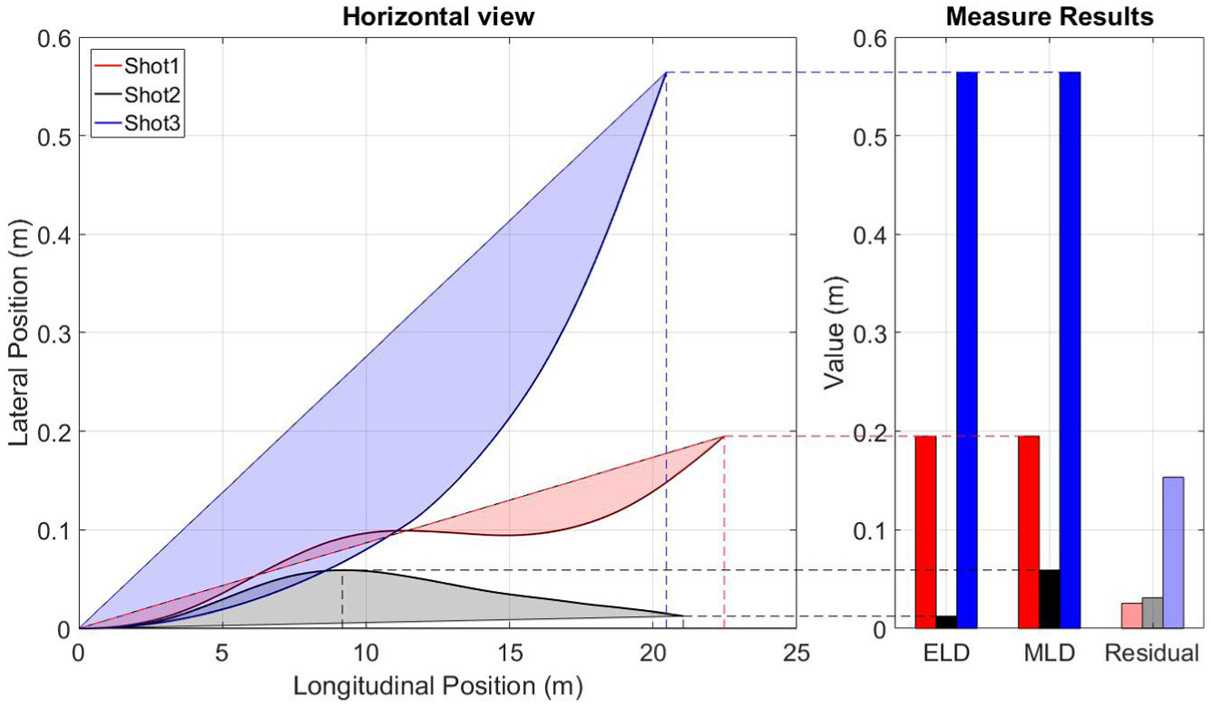
Graphical description of central tendency methods: flight paths (left) and measure results (right).

Central tendency methods are generally simple to understand and are effective at analysing the result of a shot, but do not provide sufficient detail on the shot path as a whole to draw conclusions about the general shape of the shot.

Shape profile measures

To gain an understanding of the flight path, methods must be employed that can quantify the shape or predictability of a shot. A possible measure to describe the shape of the flight is to fit low-order polynomials to the flight path. The higher the order required to effectively match the trajectory, the more irregular the flight. To calculate what order polynomial is required to adequately model the curve, increasing orders of polynomial are fitted and an arbitrary threshold value is imposed on the RMS residual error between the true flight path and fitted polynomial. Once the residuals drop below the threshold, that flight can be modelled effectively by that order polynomial. The decay of residuals with polynomial order for two shots can be seen in Figure 7. It can be seen that the more complex shot 1 requires fourth-order to effectively model, whereas shot 2 only requires a quadratic. This method will capture changes of lateral direction in flight and define the shape, but needs the central tendency measures to provide real world context.

Figure 7.

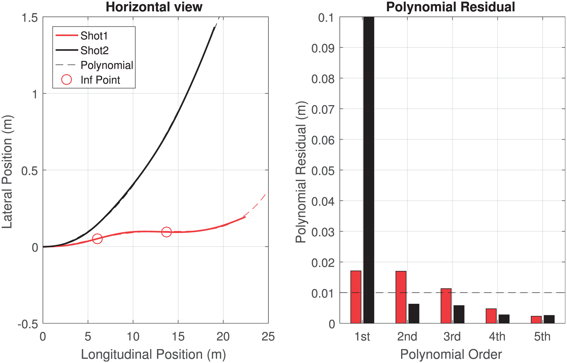
Polynomial fitting: flight paths with accepted polynomials and inflection points (left) and residual decay with increasing order (right).

Analysing the polynomial coefficients to determine the severity of change in direction was also investigated to provide more detail on the severity of the inflections. The coefficients could also be combined across the shots to build an ‘average’ shot path. While this can work well for a small number of similar runs, combining the coefficients across a wide range of shots will mask many important features of the flight, such as high-order deviations.

Another pair of measures, proposed by Rogers,¹⁷ is to count the number of inflection points and calculate an auto-correlation coefficient for the shot path. An inflection point is defined when the concavity of the line changes, in this case relative to the line drawn from the start to the finish point as shown by markers in Figure 7. The number of inflection points is a definite, easily understood result. One drawback is that there is a sensitivity to a ball oscillating closely about a central line; this would indicate a high level of instability, whereas the actual path may, from the player’s perspective, appear straight. To counteract this, Rogers used an auto-correlation method to describe the predictability of a flight path based on previous points with a low value indicating a more random flight path. For example, shot 1 has a lower auto-correlation coefficient than shot 2. This value could be used to classify the flight as having ‘major’ or ‘minor’ inflections.

Magnus deviation

The previous methods have attempted to model the flight as a whole, but do not isolate individual parts of the ball’s performance, such as the ball’s orientation dependency. To calculate this, the simulation is run twice; once with orientation-dependent forces active and once inactive, in combination with spin dependent forces. Comparing these flight paths using an RMS method will provide a direct quantification of the effect of orientation-dependent forces, which are particularly significant at lower spin rates, isolated from spin dependent forces.⁷ This is referred to as the Magnus deviation in this article. Flight paths, both with and without orientation-dependent forces in combination with spin dependent forces are shown in Figure 8. The shaded area represents the Magnus deviation value each shot would generate. Shot 1 has a very small value as the two shots follow similar paths, indicating that the orientation has little effect, either due to the ball, or a high spin rate introducing dominant Magnus forces. Shot 2 has a large value, as the orientation has a significant effect on the flight path.

Figure 8.

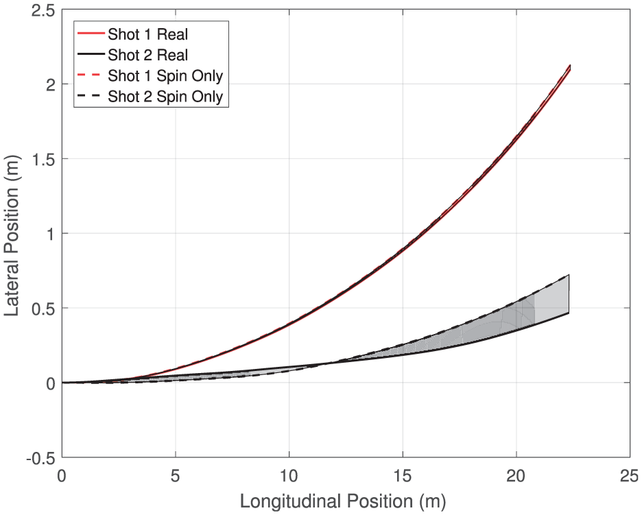
Magnus deviation example for low and high spin shots.

Normalisation

A source of bias in the ELD and MLD measurements is the distance the ball travels during flight, arising due to changes in initial velocity or launch elevation angle. A long and short shot with the same lateral movement should not be recognised as having the same characteristics. To remove this bias, these measures are each divided by the total distance the ball has travelled in the horizontal plane and expressed as the deviation per metre of flight.

Method selection

Each of these methods has its benefits and disadvantages and can be more effective at describing some types of shots than others while in some cases describing similar behaviour of the ball. To provide a concise measure of a ball’s performance, the fewest number of measures should be selected that accurately represent the ball’s overall aerodynamic performance and do not quantify the same characteristics. Cross-correlation coefficients are obtained for the seven measures described in this article and are displayed in Table 2. These are based on a set of results for the three balls obtained using the input test matrix described in this article. All three central tendency measures show high degrees of correlation, as do the polynomial order and auto-correlation coefficient, indicating that they describe similar characteristics. Therefore, to fully describe the flight, only one of each of these is required. The number of inflection points and the Magnus deviation show some correlation to the polynomial order and auto-correlation methods, but there is still value in presenting these as separate measures of the ball’s orientation dependency. This article has selected the polynomial order to model the general shape of the flight. The number of inflection points to quantify the smaller changes in direction. The ELD to provide some real-term context to these results and the Magnus deviation to characterise the orientation dependency of the ball. These have been selected as they do not correlate strongly to one another, are easy to consider in real terms and can be combined across the range of shots. The chosen parameters are in bold in Table 2.

Table 2.

Cross-correlation coefficients.

Measure	End lateral deviation	Maximum lateral deviation	RMS residual deviation	Polynomial order	Auto-correlation coefficient	Inflection points	Magnus deviation
ELD	1.000	0.995	0.953	0.771	0.743	0.402	0.511
MLD	0.995	1.000	0.961	0.770	0.744	0.416	0.497
Residual	0.953	0.961	1.000	0.735	0.667	0.362	0.535
Polynomial	0.771	0.770	0.735	1.000	0.944	0.694	0.720
Auto-correlation coefficient	0.743	0.744	0.667	0.944	1.000	0.791	0.626
Inflection points	0.402	0.416	0.362	0.694	0.791	1.000	0.430
Magnus	0.511	0.497	0.535	0.720	0.626	0.430	1.000

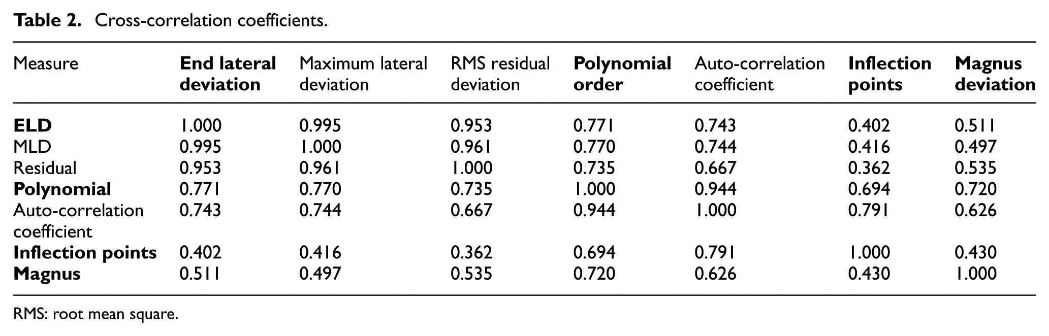
RMS: root mean square.

Result analysis

The three balls described in the wind tunnel testing section were tested using this procedure. These were FIFA approved balls with different numbers of seams and various surface texturing. For each of the shots across the full range of V, $ω, α$ , and $ψ$ , the values of the normalised ELD, the polynomial fit order, Magnus deviation, and number of inflection points were calculated and averaged and are shown in Figure 9. These values can be directly compared to other balls that have undertaken the same tests and analyses. If the ELD is high, this will indicate that the ball tends to move more in flight. The polynomial order will indicate the overall predictability of the ball in flight and the number of inflection points will define the number of changes of direction of the ball in the shot. Finally, the Magnus deviation will isolate the orientation dependency of the ball. These measures were found to vary most with spin rate, as the behaviour of the ball in flight changes significantly from low to high spin rates. Each measure is plotted against spin rate in Figure 9, such that each point represents the mean result from all the combinations of V, $α$ , and $ψ$ described in Table 1 at the given spin rate.

Figure 9.

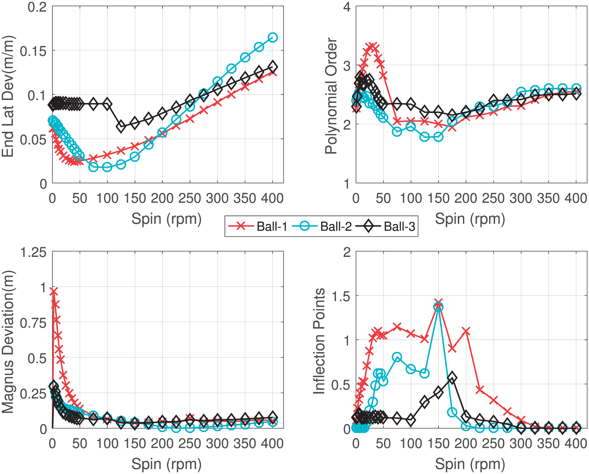
Results against spin rate for three FIFA-approved balls using the specified input conditions. Each datapoint represents the mean result for all the combinations of V, $α$ , and $ψ$ described in Table 1 at the given spin rate—top left: normalised end lateral deviation, top right: polynomial order, lower left: Magnus deviation, and lower right: inflection points.

Ball 2 had very low ELD at 100 rpm, increasing more rapidly with spin rate above this value than the other balls. Ball 1 had a comparable dip, but at a lower spin rate of 50 rpm. Ball 3 had a consistent deviation across spin rates.

Ball 1’s polynomial order was more often higher than those of the other balls at low spin rates, indicating it was the least consistent in flight. As the spin rates increased, the measures converged, indicating that the shape of the trajectory was less dependent on the ball type at higher spin rates. Ball 3 was, again, very consistent across the spin rates.

Ball 1 had the greatest Magnus deviation at low spin rates, which would indicate that its orientation forces (as shown in 1 and discussed by Passmore et al.⁷) had greater influence over the trajectory of the ball. The measurements for Balls 2 and 3 were comparable. Above 100 rpm, the orientation had less influence on the flight; this supports the findings of Passmore et al.⁷ that the orientation-dependent component of lateral forces decays with increasing spin rate.

The number of inflection points indicates that Ball 1 was least stable in flight, while Ball 3 rarely changed direction in flight, even at low spin rates.

The increased orientation sensitivity of Ball 1 suggested by the Magnus deviation correlates to less consistent flights in the polynomial order and inflection point values. This is in agreement with the conclusions drawn by Passmore et al.⁷ It can also be concluded that at higher spin rates, Ball 2 will curve the most, although it has dramatically different behaviour at 100 rpm.

For these results, the main differences occur at lower spin rates, particularly for measures of flight shape. The values tend to be more consistent for the three balls at middling to high spin rates, except for the ELD, which exhibits interesting differences between the balls.

Conclusion

This article has defined a process for characterising a footballs’ flight for a wide range of input initial conditions. These flights were generated using a 6-degree-of-freedom flight model that utilises drag and lateral forces measured in a wind tunnel for a range of speeds and spin conditions for each of the test balls.

The range of flights was analysed using a range of statistical measures applied using methods defined in the article. From the analysis, four parameters were extracted that usefully describe the overall flight behaviour, while other parameters that described similar behaviour or were less intuitive were not included in the analysis:

The ELD defined the magnitude of lateral movement.

The polynomial fit order described the underlying shape of the trajectory.

The Magnus deviation isolated the ball’s orientation dependency from spin dependent forces.

The number of inflection points defined the number of changes of direction for each flight.

The quantitative data obtained using these methods can be applied in a number of practical applications, such as ball development and evaluation processes as well as potentially for regulatory purposes. In addition, if a particular feature of the ball’s performance envelope is of interest, then the test input parameters can be deliberately adjusted to focus on specific conditions.

Further work is required to gain an understanding of the relationship between the characterisation parameters and human perceptions of ball flight performance and to understand how the physical ball features can affect the characterisation values.

Footnotes

Appendix 1 Acknowledgements

The authors thank the adidas FUTURE team for supplying the physical prototype balls and providing their support throughout the project.

Declaration of conflicting interests

The author(s) declared no potential conflicts of interest with respect to the research, authorship, and/or publication of this article.

Funding

The author(s) disclosed receipt of the following financial support for the research, authorship, and/or publication of this article: This work was supported by the Engineering and Physical Sciences Research Council.

ORCID iD

Matthew Ward

References

Passmore

Rogers

Tuplin

, et al. The aerodynamic performance of a range of FIFA approved footballs. Proc IMechE Part P: J Sports Engineering and Technology 2011; 226(1): 61–70.

FIFA. Testing and certification for footballs, international match ball standard. Zürich: FIFA, 2006.

Passmore

Tuplin

Spencer

, et al. Experimental studies of the aerodynamics of spinning and stationary footballs. Proc IMechE Part C: J Mechanical Engineering Science 2008; 222(2): 195–205.

Achenbach

. The effects of surface roughness and tunnel blockage on the flow past spheres. J Fluid Mech 1974; 65(1): 113–125.

Achenbach

. Experiments on the flow past spheres at very high Reynolds numbers. J Fluid Mech 1972; 54(3): 565–575.

Mehta

. Aerodynamics of sports balls. Ann Rev Fluid Mech 1985; 17: 151–189.

Passmore

Tuplin

Stawski

. The real-time measurement of football aerodynamic loads under spinning conditions. Proc IMechE Part P: J Sports Engineering and Technology 2016; 231: 262–274.

Carré

Goodwill

Haake

. Understanding the effect of seams on the aerodynamics of an association football. Proc IMechE Part C: J Mechanical Engineering Science 2005; 219(7): 657–666.

Barber

Chin

Carré

. Sports ball aerodynamics: a numerical study of the erratic motion of soccer balls. Comp Fluids 2009; 6(38): 1091–1100.

10.

Kim

Choi

Park

, et al. Inverse Magnus effect on a rotating sphere: when and why. J Fluid Mech 2014; 754(2): R2.

11.

Rogers

Passmore

Harland

, et al. An experimental validation method of wind tunnel measurements on FIFA approved footballs using kicking tests in wind-free conditions. In: Sabo

Litzenberger

Kafka

, et al. (eds) 8th conference of the international sports engineering association. Vienna: Procedia Engineering, pp 2481–2486.

12.

Bray

Kerwin

. Modelling the flight of a soccer ball in a direct free kick. J Sports Sci 2003; 21: 75–85.

13.

Ronkainen

Holmes

Harland

, et al. A comparative study of ball launch measurement systems; soccer case study. In: Estivalet

Brisson

(eds) 7th conference of the international sports engineering association. Biarritz: Springer, pp 239–246.

14.

Asai

Seo

. Aerodynamic drag of modern soccer balls. Springerplus 2013; 2: 171.

15.

Murakami

Kondoh

Iwai

, et al. Measurement of aerodynamic forces and flow field of a soccer ball in a wind tunnel for knuckle effect. In: Sabo

Litzenberger

Kafka

, et al. (eds) 8th conference of the international sports engineering association. Vienna: Procedia Engineering, pp 2467–2472.

16.

Hong

Sakamoto

Washida

, et al. The influence of panel orientation on the aerodynamics of soccer balls. In: James

Wheat

Choppin

, et al. (eds) The 2014 conference of the international sports engineering association. Sheffield: Procedia Engineering, pp 786–791.

17.

Rogers

. A study of the relationship between surface feature and the in-flight performance of footballs. PhD Thesis, Loughborough University, Loughborough, 2011, dspace.lboro.ac.uk/dspace-jspui

18.

Johl

Passmore

Render

. The design methodology and performance of an in-draft wind tunnel. Aeronaut J 2004; 108(1087): 465–473.

19.

Sawada

Suda

. Study on aerodynamic force acting on a sphere with and without boundary layer trips around the critical Reynolds number with a magnetic suspension and balance system. Exp Fluids 2011; 50: 271–284.

20.

Myers

Mitchell

. A mathematical analysis of the motion of an in-flight soccer ball. Sports Eng 2013; 16(1): 29–41.

21.

Tuplin

Passmore

Rogers

, et al. The application of simulation to the understanding of football flight. Proc IMechE Part P: J Sports Engineering and Technology 2012; 226(2): 134–142.

22.

Carré

Asai

Akatsuka

, et al. The curve kick of a football II: flight through the air. Sports Eng 2002; 5(4): 193–200.

23.

Shinkai

Nunome

Isokawa

, et al. Ball impact dynamics of instep soccer kicking. Med Sci Sports Exer 2009; 41(4): 889–897.

Characterisation of football trajectories for assessing flight performance

Abstract

Keywords

Introduction

Background

Characterisation procedure

Experimental method

Wind tunnel measurements

Flight model

Input parameters

Flight characterisation techniques

Central tendency measures

Shape profile measures

Magnus deviation

Normalisation

Method selection

Result analysis

Conclusion

Footnotes

Appendix 1

Acknowledgements

Declaration of conflicting interests

Funding

ORCID iD

References