For scientists conducting research, fractional integral differential equation analysis is crucial. Therefore, in this study, we investigate analysis utilizing a novel method called the fractional decomposition method, which is applicable to fractional nonlinear fractional Fredholm integro-differential equations. Then, we apply the approach to five test problems for a general fractional derivative involving fractional Fredholm integro-differential equations. To the best of our knowledge, we are the first to ever do so because of the very complicated calculations involved when dealing with the general case . For fractional Fredholm integral-differential equations, we provide both exact and approximate solutions. Throughout this work, the fractional Caputo derivative is discussed. This technique leads us to say that the method is precise, accurate, and efficient, according to the theoretical analysis.
Fractional integro-differential equation (FIDE) is used in a variety of scientific fields, including demography, insurance mathematics, and physics.1–5 Any IVP or BVP that is converted to an IE typically produces an integral-differential equation (IDE), which may be seen in a variety of scientific models.6,7 Many integro-differential equations contain both integral and differential operators. As a result, we must look for an effective method for locating analytical solutions to fractional differential equations.
Due to their usefulness in several disciplines of science and engineering, FIDEs have attracted the attention of numerous researchers in recent years.8–17 in particular, fractional Volterra and Fredholm FIDEs.
The research community is aware of many methods to handle FIDE. To name a few, the fractional decomposition method (FDM),18–22 the fractional adomian decomposition method,23,24 the interpolation correction for collocation,6 the second-kind Chebyshev wavelet,7,8 the least squares method and shifted Laguerre polynomials pseudo-spectral method,15 the spectral-collocation method,11 the Taylor expansion method,12 the cubic b-spline operational matrix,13 and the13 are recent examples of effective and dependable techniques9,16 are recent examples of effective and dependable techniques.15 Additionally, M. Rawashdeh has produced additional theorems that support utilizing the FNDM to obtain analytical approximations of solutions to fractional nonlinear PDEs. They were the first researchers to integrate both the natural decomposition technique and the adaptive decomposition technique to solve linear and nonlinear ODEs and PDEs in a thesis written by S. Maitama in 2014 and the first author of the current work.
We use the newly developed approaches (FDM) to five linear and nonlinear Fredholm integro-differential equations in order to demonstrate the viability and efficiency of our new approach, which will also demonstrate the ease and simplicity of the current procedure.
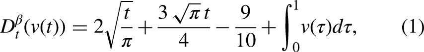
First, we explore the linear fractional Fredholm integro-differential equations (FFIDE) with given by:
a company with its IC:
It is known that is the exact solution when of the above equation (1).
Second, we take a look at the linear FFIDE given by:
a company with its I.C:
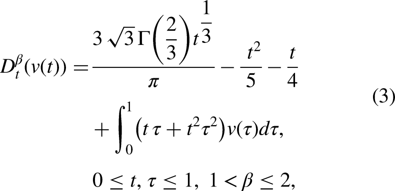
Third, we examine the nonlinear FFIDE with given as:
a company with its I.C:
Fourth,we explore the nonlinear FFIDE given as:
a company with its I.C:
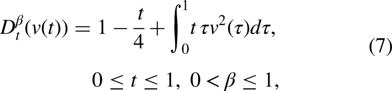
Finally, we inspect the nonlinear FFIDE given as:
a company with its I.C:
The current research work is presented as follows: Definitions and some background information about fractional calculus are presented in the ‘Fractional Calculus Background’ section. ‘The natural-adomian method’ section is devoted to some theories of N-transformation as well as some significant properties of the natural transform. The convergence study of the FDM used with the nonlinear FFIDE is thoroughly examined in the ‘Convergence Analysis of the FDM for nonlinear FFIDE’ section. In the ‘Numerical results and applications’ section, we apply the FDM to five linear and nonlinear FFIDEs. The ‘Concluding Remarks’ section will serve as the conclusion to the current work.
Fractional Calculus Background
We begin by going over some crucial concepts and properties that are helpful whenever someone discusses the topic of fractional calculus.1–5
If , where . Then is in the space if such that , where in , and if .
The Riemann-Liouville fractional integral for a function of order , is defined as:
The Caputo fractional derivative of is given by:
for .
The Gamma function can be defined as:
Given a complete metric space. Then is called a contraction mapping on if we can find a such that , for all .
Given complete nonempty metric space , and is a contraction mapping, then has a unique fixed-point, such that .
Given a non-empty complete metric space with a map which is of a contraction type. Then the mapping has a unique fixed-point (i.e. ). Furthermore, can be found as follows: start with an arbitrary element and define a sequence by for . Then .
The natural-adomian method
We recommend that readers learn more about the history of the general integral transform, the Laplace, Sumudu, and natural transform methods, as well as their related properties, for any given function , , see for example.25–27
Let be a piece-wise continuous function on . If with , define So, for i.e. and for i.e. .
Note that for any in the class with we have:
Which is convergent provided that and , which implies that i.e. . Loosely speaking, is a function of exponential order.
Then, one can define the natural transformation (N-transformation) as:
where is the N-transform of and and are the N-transform variables. Note that one can write Equation (refeq3.1) as,
where,
Moreover,
Thus, equation (15) is the natural transformation and equation (16) is the inverse natural transformation.
We will use the following helpful N-transforms properties throughout this paper, see Abassy24, Belgacem25 and Bulut et al.26:
.
Suppose that , where and is the natural transformation of the function , then the natural transformation of the fractional derivative in the Caputo sense of the function of order denoted by is given by:
Convergence analysis of the FDM for nonlinear FFIDE
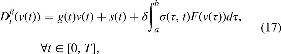
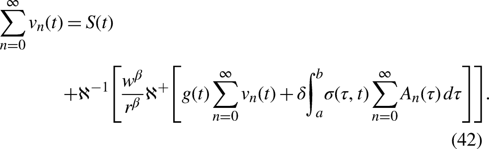
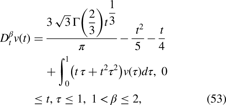
In this section, we first give proofs for the uniqueness and convergence theorems, and then we give an error estimate using the FDM. Consider the general nonlinear nonhomogeneous FFIDEs:
where .
Along with I.C:
Note that the fractional derivative of the function is in the sense of Caputo, is a nonlinear continuous function and is the non-homogeneous term and .
Employ the N-transformation and property 4 to equation (17) to find:
So,
Thus,
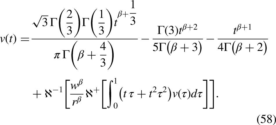
Take the inverse of N-transform to find:
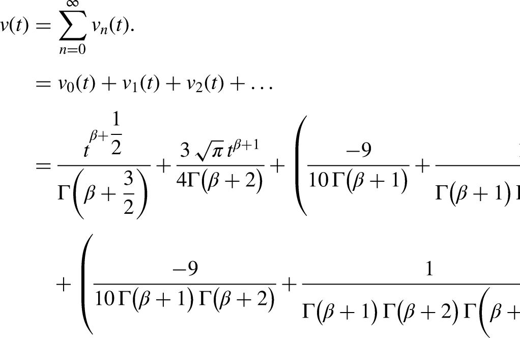
Suppose our solution of given by:
Moreover, the nonlinear part is written as:
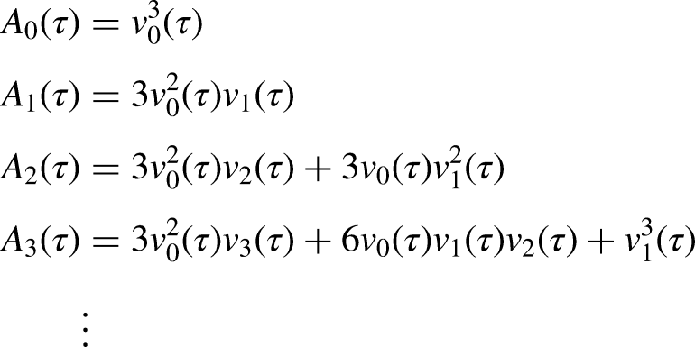
Note that the Adomian polynomial of are represented by ’s which can be computed by:
Note that we can simplify the formula in equation (25) to be:
We can continue in this manner to get the other polynomials.
Substitute equation (23) into equation (22) to arrive at:
Note that represents the initial conditions and the non-homogeneous part. We shall use the new form of Adomian polynomials, see Adomian23 and Abassy24 to find:
, where .
(Uniqueness Theorem). Let with . Then equation (17) has a unique solution.
Consider the Banach space of all functions on which are also continuous, say having a norm . Let be define by:
Assume and . Further, suppose and , where are the Lipschitz constants and are two different solutions of equation (17).
Since , then is contraction mapping and it follows by Theorem (2), then there exists unique solution to equation (17). □
(Theorem of Convergence). The series solution in equation (30) of equation (17) using the FDM converges provided that and .
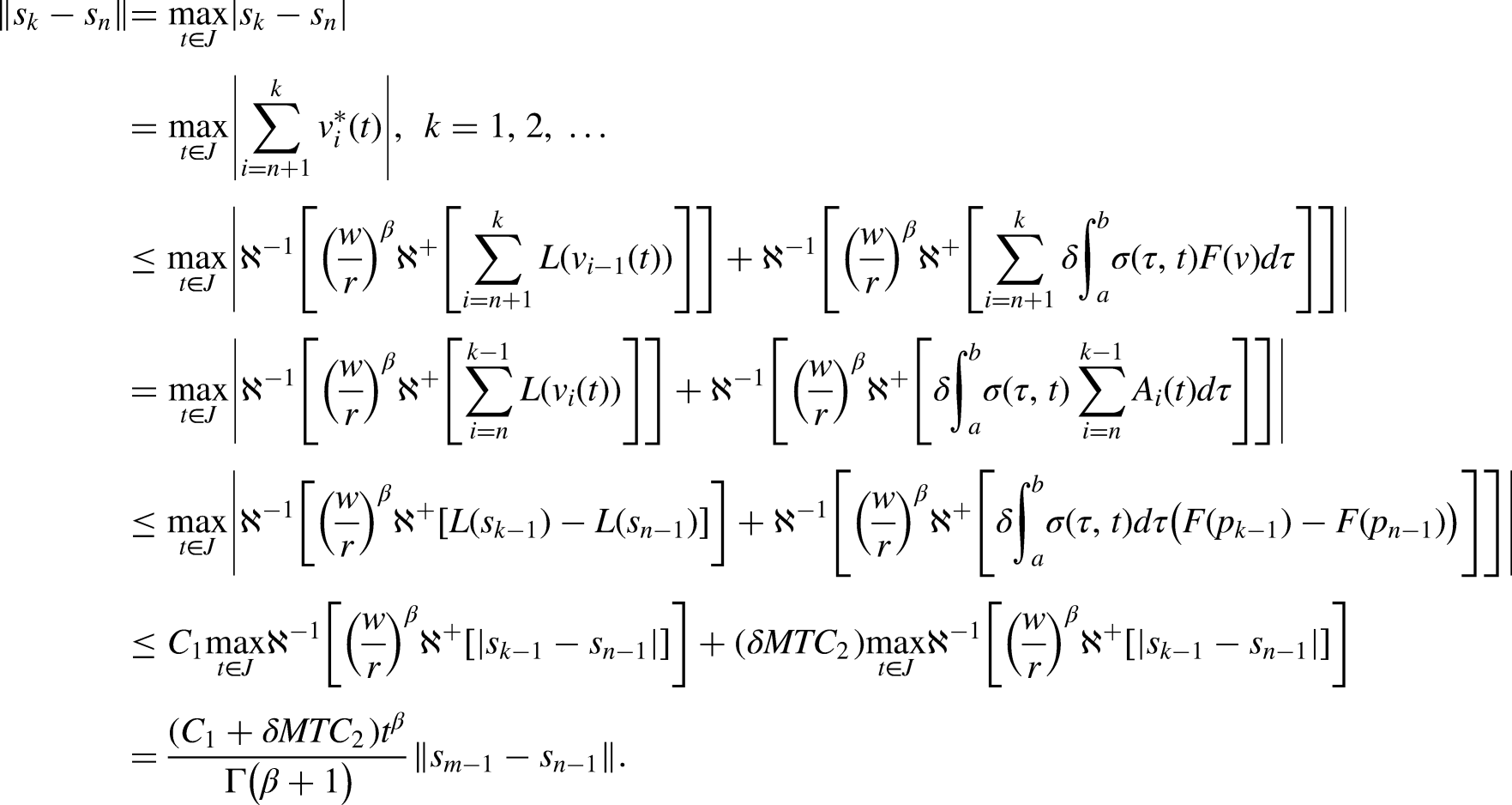
Consider the to be the m-th partial sum, i.e. . We need to show that is a Cauchy sequence in the Banach space . Consider the new formulation of the Adomian polynomials mentioned: . Let and be any two partial sums with . Then,
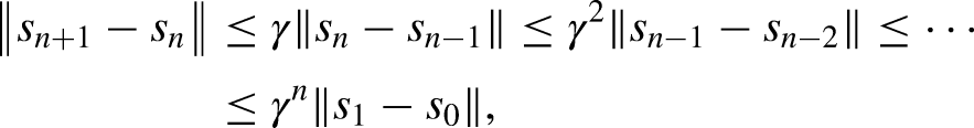
Thus, . Choose , then
where .
Similarly, using the triangle inequality
But, , then . Thus,
Since is bounded, then . So, as , then . Thus, the sequence is a Cauchy in . Hence, converges. □
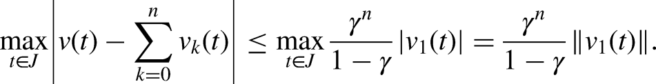
(Estimating the Error). The maximum absolute truncation error of the series solution in Equations (17) to (30) is estimated to be
From Equation (31) in Theorem 4 we conclude that . So as , we have . Then . Therefore, the maximum absolute truncation error in is:
□
Numerical results and applications
In this section, we apply the FDM to five examples and compare the approximate solutions to the exact solutions that are already in place. First, we present the methodology of the FDM: Consider the general nonlinear FFIDEs with initial conditions given by:
A company with I.Cs:
Note that the fractional derivative is in the Caputo sense of , is a nonlinear continuous function and is the non-homogeneous term.
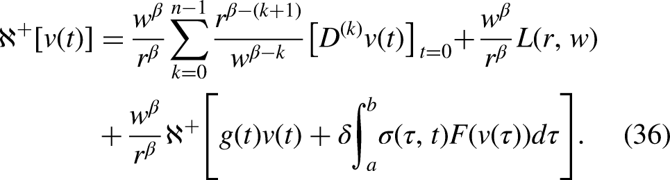
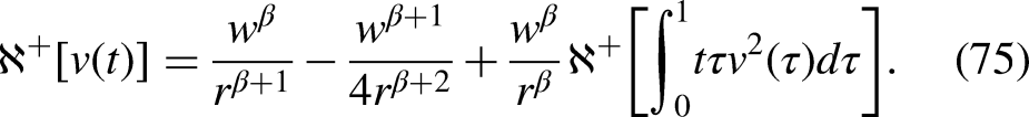
Employing the natural transformation and property (4) to equation (32), we arrive at:
Thus,
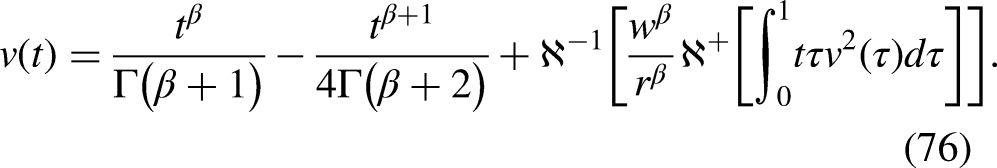
Substituting equation (33) into equation (36) and applying the inverse transform to equation (36), we arrive at:
Here the non-homogeneous part and the I.Cs are represented by . Suppose our intended solution is given by:
Also, the nonlinear term is:
Here, ’s are the polynomials of which can be calculated using:
From equation (67), one can write equation (66) as:
Note that is the Adomian polynomial which represents the nonlinear part.
Note that:
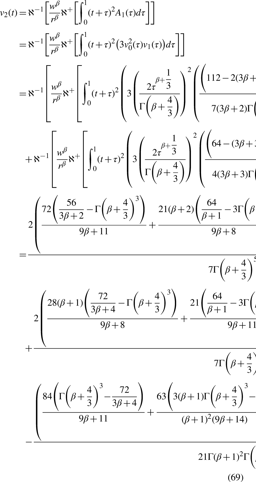
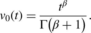
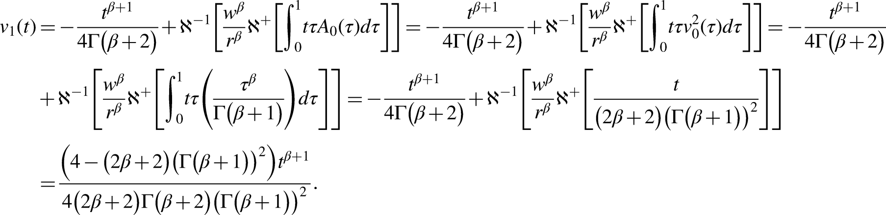
Looking at equation (68) above, one can calculate the iterations as:
And,
Thus,
It is worth mentioning here because this iteration, , is almost three pages; we didn’t include it in the text of the paper, but when we sketched the graph and did the table, we included it in the Mathematica file, and it is available.
Hence,
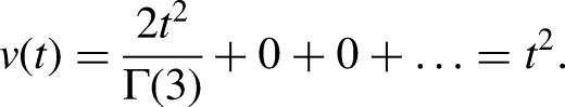
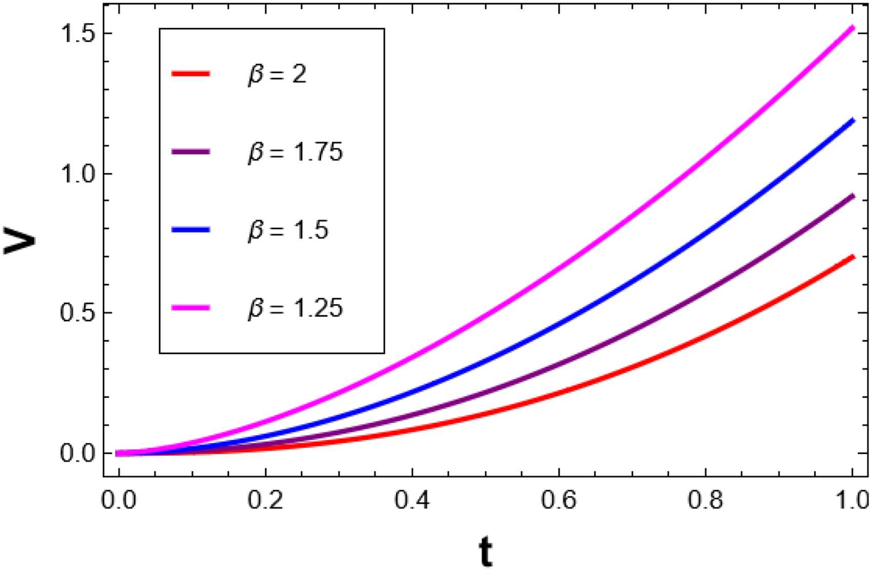
When , we get
Which is in fact the exact solution for equation (61) in the special case .
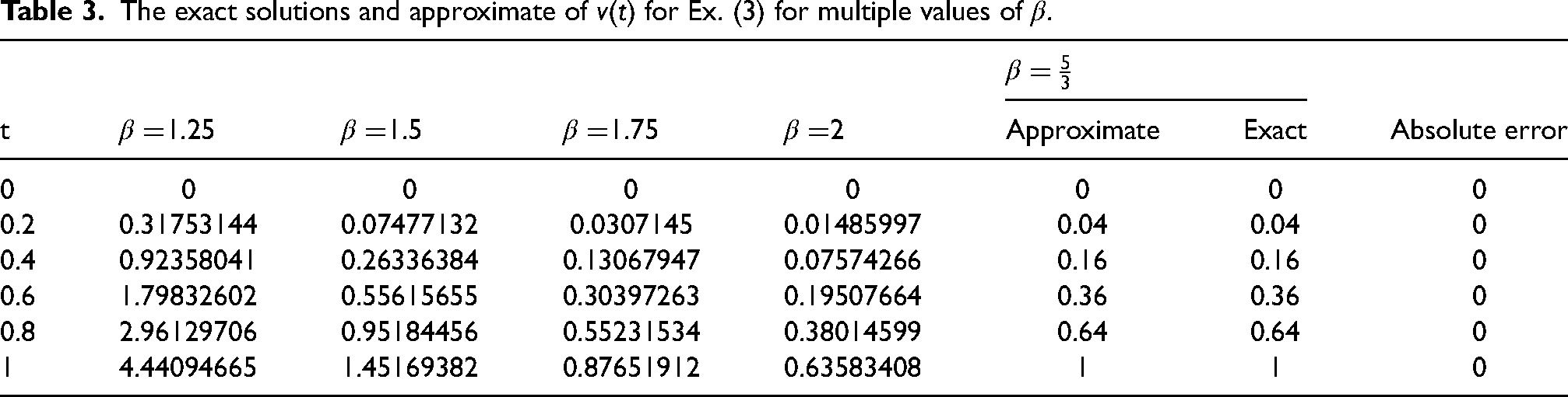
Choosing β = {1.25, 1.5, 1.75, 2} in the above equation, we find Figure 3 and Table 3 below:
Numerical values for of Ex. (3) for multiple values of when .
The exact solutions and approximate of for Ex. (3) for multiple values of .
t
1.25
1.5
1.75
2
Absolute error
Approximate
Exact
0
0
0
0
0
0
0
0
0.2
0.31753144
0.07477132
0.0307145
0.01485997
0.04
0.04
0
0.4
0.92358041
0.26336384
0.13067947
0.07574266
0.16
0.16
0
0.6
1.79832602
0.55615655
0.30397263
0.19507664
0.36
0.36
0
0.8
2.96129706
0.95184456
0.55231534
0.38014599
0.64
0.64
0
1
4.44094665
1.45169382
0.87651912
0.63583408
1
1
0
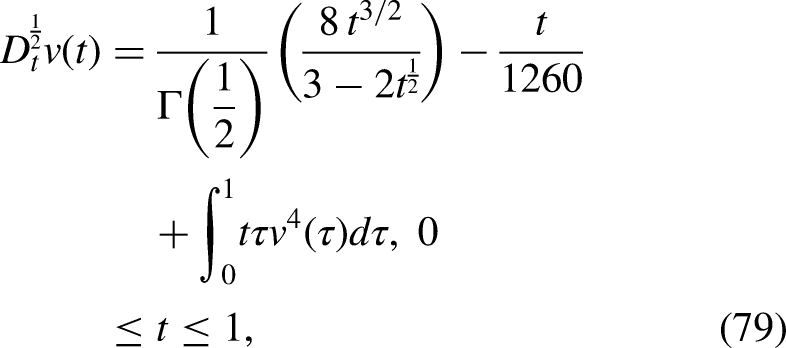
Given the nonlinear FFIDE:
together with I.C:
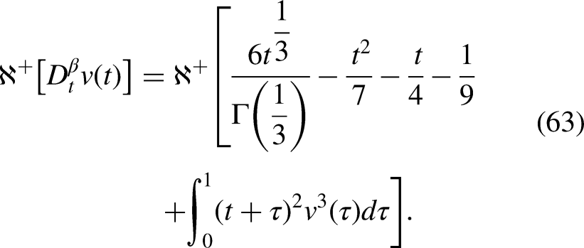
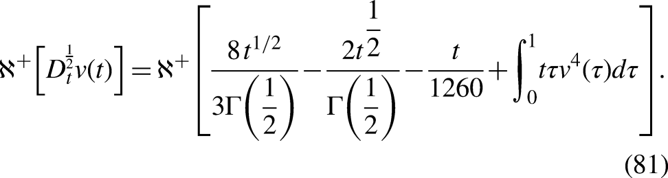
Solution: Using N-transformation of equation (71) to find:
Now using property 4 we get:
Substitute equation (72) into equation (74) to find:
From equation (85), one can write equation (84) as:
Note that, is the Adomian polynomial which represents the nonlinear part.
Note that
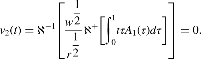
Looking at equation (75) above, one can calculate the remaining iterations as:
And,
So,
Thus, one can concludes that
Hence,
Which is in fact the exact solution for equation (79).
Concluding remarks
The FDM for nonlinear FFIDE convergence analysis was successfully adopted in the current study work. Additionally, we discovered approximate and analytical solutions to the fractional linear and nonlinear Fredholm integro-differential equations. The new method reduces the calculation challenges of some of the well-known and famous methods and allows for simple computations. Utilizing the FDM, some well-known FFIDE applications were investigated, and the results revealed distinct disparities. Without any linearization, discretization, or perturbation, the employed technique can be applied to a variety of linear and nonlinear FFIDEs. Our long-term goals are to use FDM to solve various linear and nonlinear FFIDEs that appear in many branches of applied research, such as physics and engineering.
Footnotes
Acknowledgement
The author(s) would like to send our thanks to the reviewers for finding the time to read and improve our work in the current manuscript.
Declaration of conflicting interests
The author(s) declared no potential conflicts of interest with respect to the research, authorship, and/or publication of this article.
Consent to participate
Participants are aware that they can contact the Jordan University of Science and Technology Ethics Officer if they have any concerns or complaints regarding the way in which the research is or has been conducted.
Funding
The authors received no financial support for the research, authorship and/or publication of this article.
ORCID iD
Mahmoud S Rawashdeh
References
1.
CaputoM. Elasticita e dissipazione. Bologna: Zanichelli, 1969.
2.
HilferR Ed. Applications of fractional calculus in physics. Germany: World scientific, Universität Mainz & Universität Stuttgart, 2000.
3.
KilbasAASrivastavaHMTrujilloJJ. Theory and applications of fractional differential equations, Vol. 204. Amsterdam: Elsevier, 2006.
4.
MillerKSRossB. An introduction to the fractional calculus and fractional differential equations. New York, NY, USA: Wiley, 1993.
5.
PodlubnyI. Fractional differential equations: an introduction to fractional derivatives, fractional differential equations, to methods of their solution and some of their applications. Vol. 198. Elsevier, 1998.
6.
HuQ. Interpolation correction for collocation solutions of fredholm integro-differential equations. Math Comput Am Math Soc1998; 67: 987–999.
7.
ZhuLFanQ. Solving fractional nonlinear fredholm integro-differential equations by the second kind chebyshev wavelet. Commun Nonlinear Sci Numer Simul2012 Jun 1; 17: 2333–2341.
8.
SetiaALiuYVatsalaAS. Solution of linear fractional Fredholm integro-differential equation by using second kind Chebyshev wavelet. 2014 11th International Conference on Information Technology: New Generations. IEEE, 2014.
9.
ArikogluAOzkolI. Solution of fractional integro-differential equations by using fractional differential transform method. Chaos, Solitons Fractals2009; 40: 521–529.
10.
DaraniaPEbadianA. A method for the numerical solution of the integro-differential equation. Appl Math Comput2007; 188: 657–668.
11.
YangYChenYHuangY. Spectral-collocation method for fractional fredholm integro-differential equations. J Korean Math Soc2014; 51: 203–224.
12.
HuangLLiXFZhaoYet al. Approximate solution of fractional integro-differential equations by taylor expansion method. Comput Math Appl2011; 62: 1127–1134.
13.
MesgaraniHSafdariıHGhasemianAet al. The cubic B-spline operational matrix based on haar scaling functions for solving varieties of the fractional integro-differential equations. J Math2019; 51: 45–65. (ISSN 1016-2526).
14.
HamoudAAAbdoMSGhadleKP. Existence and uniqueness results for caputo fractional integro-differential equations. J Korean Soc Indu Appl Math2018; 22: 163–177.
15.
MahdyAMShwayyeaRT. Numerical solution of fractional integro-differential equations by least squares method and shifted laguerre polynomials pseudo-spectral method. Int J Sci Eng Res2016; 7: 1589–1596.
16.
NazariDShahmoradS. Application of the fractional differential transform method to fractional-order integro-differential equations with nonlocal boundary conditions. J Comput Appl Math2010; 234: 883–891.
17.
MohammedDS. Numerical solution of fractional integro-differential equations by least squares method and shifted chebyshev polynomial. Math Probl Eng2014; 2014: 1–5.
18.
RawashdehMSAl-JammalH. New approximate solutions to fractional nonlinear systems of partial differential equations using the FNDM. Adv Differ Equ2016; 2016: 1–19.
19.
RawashdehMS. The fractional natural decomposition method: Theories and applications. Math Methods Appl Sci2017; 40: 2362–2376.
20.
ObeidatNABentilDE. New theories and applications of tempered fractional differential equations. Nonlinear Dyn2021; 105: 1689–1702.
21.
ObeidatNABentilDE. Convergence analysis of the fractional decomposition method with applications to time-fractional biological population models. Numer Methods Partial Differ Equ2023; 39: 696–715.
22.
ObeidatNABentilDE. Novel Technique to Investigate the Convergence Analysis of the Tempered Fractional Natural Transform Method Applied to Diffusion Equations. In Press June 5, 2022, in the Journal of Ocean Engineering and Science. doi:10.1016/j.joes.2022.05.014.
23.
AdomianG. A review of the decomposition method in applied mathematics. J Math Anal Appl1988; 135: 501–544.
24.
AbassyTA. New treatment of adomian decomposition method with compaction equations. Stud Nonlinear Sci2010; 1: 41–49.
25.
BelgacemFBMSilambarasanR. Theory of natural transform. Math Engg Sci Aeros2012; 3: 99–124.
26.
BulutHBaskonusHMBelgacemFBM. The analytical solution of some fractional ordinary differential equations by the Sumudu transform method. Abstract and Applied Analysis. Vol. (2013), Hindawi, 2013.
27.
LoonkerDBanerjiPK. Natural transform and solution of integral equations for distribution spaces. Am J Math Sci2014; 3: 65–72.