Sage Journals: Discover world-class research

Abstract

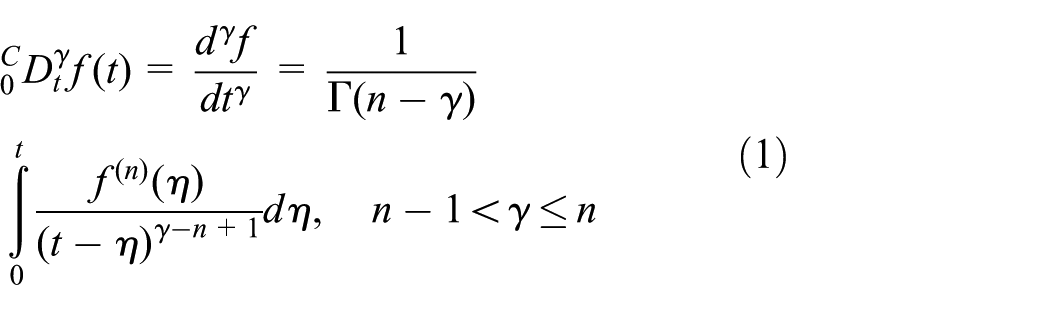
In this article, we obtain the viscous damping coefficient β theoretically and experimentally in the spring–mass–viscodamper system. The calculation is performed to obtain the quasi-period τ. The influence of the viscosity of the fluid and the damping coefficient is analyzed using three fluids, water, edible oil, and gasoline engine oil SAE 10W-40. These processes exhibit temporal fractality and non-local behaviors. Our general non-local damping model incorporates fractional derivatives of Caputo type in the range $(0, 1]$ , and the viscous damping coefficients are determined in terms of the inverse Mittag-Leffler function. The classical models are recovered when the order of the fractional derivatives is equal to 1.

Keywords

Fractional calculus Caputo fractional derivative inverse Mittag-Leffler function fractional-order damping mass–spring–damper system

Introduction

In recent years, the representation of physical models based on non-integer order derivative has attracted a considerable interest due to the fact that these models can describe memory and the hereditary properties of various materials and processes.^1–6 For example, fractional derivatives have been used successfully to model viscoelastic behavior of materials,⁷ frequency-dependent damping behavior,^8–14 viscoelastic single-mass systems,¹⁵ and viscoelasticity and anomalous diffusion.^16–19 Also, they are used in modeling of chemical processes, control theory, electromagnetism, thermodynamics, and many other problems in physics, engineering, and the various works cited therein.^20–23

The spring–mass–viscodamper system is a dynamic system that provides a stage of minimal complexity to essentially study all the phenomena of mechanical vibrations. In this context, some researches concerning classical mechanics introduced fractional-order derivatives, for example, Kutay and Ozaktas²⁴ investigated the relationship of the Fourier transform of fractional order to harmonic oscillation. Ryabov and Puzenko²⁵ studied the fractional oscillator engaging the Riemann–Liouville fractional derivative. Caputo²⁶ studied the classic second-order differential equation of the damped oscillator; using this model, the author quantifies the response and the decaying oscillations of a seismograph; applying the fractional calculus (FC) approach, this model introduces the mathematical memory operator represented by the fractional-order derivative in order to model realistically the response curve of more complex instruments. Stanislavsky²⁷ dealt with generalization of the mechanical oscillator using fractional derivatives. Naber²⁸ found the analytical solution of the damped oscillator fractional equation using the Caputo derivative. The analytical solution of fractional systems mass–spring and spring–damper system formed using Mittag-Leffler function was analyzed in Gómez-Aguilar et al.²⁹

Based on this system, movements of structures in an earthquake can be studied.^30–32 It is the basis for studying more complex dynamics, for example, floating structures could be an offshore floating structure or floating wind turbine;^33,34 for all these cases, it is necessary to determine the coefficient of viscous damping.³² FC has been used successfully to model applications in many branches of engineering, particularly for the design of rail pads, the dynamic analysis was conducted examining a spring–damper–mass system.³⁵ In this article, we are interested in applying FC for evaluating the damping coefficient β, in the fractional underdamped oscillator. The article is organized as follows: in section “Basic tools,” we give basic tools of FC; in section “The fractional damping model,” we present the fractional damping model. Then we present in section “Experimental setup” the experimental setup, and finally section “Conclusion” presents the conclusions.

Basic tools

Consider the space $A C^{n} [0, T]$ of functions with absolutely continuous derivative up to order $n - 1$ and with absolutely continuous $n - 1$ derivative. The Caputo fractional derivative of a function $f \in A C^{n} [0, T], T > 0$ is defined by³

{{}_{0}^{C}D}_{t}^{γ} f (t) = \frac{d^{γ} f}{d t^{γ}} = \frac{1}{Γ (n - γ)} \int_{0}^{t} \frac{f^{(n)} (η)}{{(t - η)}^{γ - n + 1}} d η, n - 1 < γ \leq n

(1)

where $n = 1, 2, \dots, \in N$ and γ is the order of the fractional derivative. From equation (1), it follows that the derivative of a constant is 0 and the initial conditions for the fractional-order differential equations can be given in the same manner as for the ordinary differential equations with a known physical interpretation, unlike other definitions of fractional derivatives.¹ Caputo derivative implies a memory effect by means of a convolution between the integer order derivative and a power of time. For this reason, in this article we prefer to use the Caputo fractional derivative.

Mittag-Leffler function has caused extensive interest among physicists due to its vast potential of applications describing realistic physical systems with memory and delay. A two-parametric function of the Mittag-Leffler type is defined by the series expansion as³

E_{γ, β} (z) = \sum_{k = 0}^{\infty} \frac{z^{k}}{Γ (γ k + β)}, (γ > 0, β > 0)

(2)

In general, z is a complex quantity. When $γ = 1$ and $β = 1$ , we have, $e^{z}$ ; therefore, the Mittag-Leffler function is a generalization of the exponential function. Some common Mittag-Leffler functions are³⁶

E_{1} (\pm z) = e^{\pm z}

(3)

E_{2} (- z^{2}) = \cos (z)

(4)

E_{3} (z) = \frac{1}{2} [e^{z^{1 / 3}} + 2 e^{- (1 / 2) z^{1 / 3}} \cos (\frac{\sqrt{3}}{2} z^{1 / 3})]

(5)

E_{4} (z) = \frac{1}{2} [\cos (z^{1 / 4}) + \cosh (z^{1 / 4})]

(6)

The Laplace transform for the Mittag-Leffler function is given as

\begin{array}{l} \int_{0}^{\infty} e^{- s t} t^{γ m + β - 1} E_{γ, β}^{(m)} (\pm a t^{γ}) d t \\ = \frac{m! s^{γ - β}}{{(s^{γ} \pm a)}^{m + 1}} (Re (s) > a^{1 / γ}) \end{array}

(7)

Then, the inverse Laplace transform has the form

L^{- 1} [\frac{m! s^{γ - β}}{{(s^{γ} \pm a)}^{m + 1}}] = t^{γ m + β - 1} E_{γ, β}^{(m)} (\pm a t^{γ})

(8)

From this expression, we have

L [{{}_{0}^{C}D}_{t}^{γ} f (t)] = s^{γ} F (s) - s^{γ - 1} f (0), 0 < γ \leq 1

(9)

The fractional damping model

The spring–mass–viscodamper system considered in this article is shown in Figure 1

Figure 1.

Mechanical oscillator considered; m is the mass, the viscous damping coefficient is β, and the spring constant is k.

Equation (10) corresponding to the mechanical system

m \frac{d^{2} y (t)}{d t^{2}} + β \frac{dy (t)}{dt} + ky (t) = 0

(10)

In previous studies of the fractional mass–spring–viscodamper system, the authors did not consider the physical dimensionality of the solutions. An alternative procedure for constructing fractional differential equation was reported in Gómez-Aguilar et al.²⁹ and successfully applied in Gómez-Aguilar and colleagues.^37,38 In this context, to keep the dimensionality of the fractional differential equation, a new parameter σ was introduced in the following way

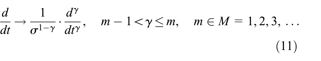
\frac{d}{dt} \to \frac{1}{σ^{1 - γ}} \cdot \frac{d^{γ}}{d t^{γ}}, m - 1 < γ \leq m, m \in M = 1, 2, 3, \dots

(11)

and

\frac{d^{2}}{d t^{2}} \to \frac{1}{σ^{2 (1 - γ)}} \cdot \frac{d^{2 γ}}{d t^{2 γ}}, m - 1 < γ \leq m, m \in M = 1, 2, 3, \dots

(12)

where γ represents the order of the fractional temporal operator and σ has the dimension of seconds; this auxiliary parameter is associated with the temporal components in the system (these components change the time constant of the system).²⁹ Ertik et al.³⁹ used the Planck time, $t_{p} = 5.39106 \times 10^{- 44} s$ , with the finality to preserve the dimensional compatibility. Following Ertik et al.,³⁹ the σ parameter corresponds to the $t_{p}$ in our calculations. For the case $γ = 1$ , expressions (11) and (12) become ordinary temporal operators. Following this idea, the fractional equation of the mass–spring–viscodamper system represented in Figure 1 is given by

{\frac{m}{{t_{p}}^{2 (1 - γ)}}}_{0}^{C} D_{t}^{2 γ} y (t) + {\frac{β}{{t_{p}}^{1 - γ}}}_{0}^{C} D_{t}^{γ} y (t) + ky (t) = 0, 0 < γ \leq 1

(13)

where the mass is m, the viscous damping coefficient is β, and the spring constant is k.

Equation (13) may be written as follows

{{}_{0}^{C}D}_{t}^{2 γ} y (t) + {λ_{γ}}_{0}^{C} D_{t}^{γ} y (t) + ω_{γ}^{2} y (t) = 0, 0 < γ \leq 1

(14)

where

λ_{γ} = \frac{β}{2 m} {t_{p}}^{1 - γ}, ω_{γ}^{2} = \frac{k}{m} {t_{p}}^{2 (1 - γ)}

(15)

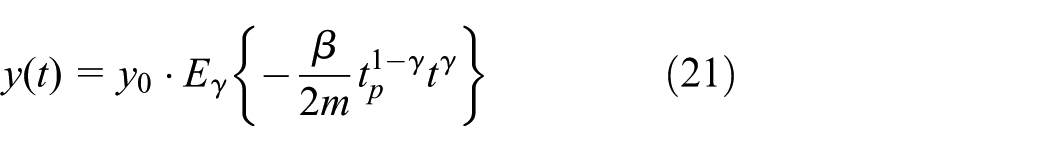
The solution of equation (14) is

y (t) = y_{0} \cdot E_{γ} {- \frac{β}{2 m} {t_{p}}^{1 - γ} t^{γ}} \cdot E_{2 γ} {- [\frac{k}{m} - \frac{β^{2}}{4 m^{2}}] {t_{p}}^{2 (1 - γ)} t^{2 γ}}

(16)

where $E_{γ, 1}$ is given by equation (2).

For the classical case $(γ = 1)$ , expression (16) becomes

y (t) = y_{0} \cdot \exp (- \frac{β}{2 m} t) \cdot \cos (\sqrt{\frac{k}{m} - \frac{β^{2}}{4 m^{2}}} t)

(17)

Experimental setup

First, consider the influence of the viscosity of the water; Figure 2 shows the system used. For this system, the mass m, measured in kilograms, is considered as the sum of the weight of the mass, denoted by $m_{1}$ , and its rod with disk (damper elements), denoted by $m_{2}$ . A bascule is used to determine $m_{1} = 0.20470 kg$ and $m_{2} = 0.015 kg$ . So $m = m_{1} + m_{2} = 0.2197 kg$ .

Figure 2.

Mechanical oscillator used in the laboratory.

The spring constant k is measured (N/m); it is determined by measuring the elongation produced by the weight of the mass m. In view of Hooke’s law, only mass $m_{1}$ is used; that is, disengaged from the damping system. This does not introduce any measurement error for the force with which the spring pulls the mass is proportional to the weight. It is denoted by $f_{r}$ force with which the spring pulls or pushes m. Therefore, $f_{r} = kx$ . The spring without deforming measured 25.5 cm; when the mass $m_{1} = 0.2047 kg$ is placed, it pulls with a force equal to its weight $W = 2.01 N$ , then the spring measured 110.8 cm. Elongation $Δ x = 110.8 - 25.5 cm$ and $Δ x = 0.853 m$ . Then, $k = 2.01 / 0.853$ ; finally, $k = 2.35 N / m$ .

The viscous damping coefficient β (measured in N s/m) is a theoretical parameter able to explain the energy dissipation due to friction that slows motion. It is not an actual physical parameter as the mass m and k spring constant, which can be accessed with a simple measurement.

The methodology followed to find an approximate value is described. In order to make time for which the mass passes through its equilibrium, we have attached a thin cardboard of negligible weight in the center of mass (whose shape is cylindrical). With the help of a timer, a piece of cardboard with dimensions of width 5 mm, length 5 cm, and thickness 1 mm and a laser measure the time it takes to move the mass break even; since the beginning of the experiment until it became indistinguishable to our measuring instruments, we take the time when the laser had an impact on the cardboard. The laser is placed in front of the mass–spring–damper system so that the laser beam formed an angle of 90° to the imaginary vertical line where the movement of the mass happens. The beam of light fell directly on the cardboard when the mass was at rest; see Figure 2.

Here, we show how we determined the viscous damping coefficient for water-based buffer, and for the other two, based on edible oil and motor oil, we did the same. For the first experiment (using water-based damper), Table 1 shows the different times for which the mass passes through its equilibrium.

Table 1.

Different times for which the mass passes through its equilibrium using the water-based damper.

$t_{1} = 0.39$	$t_{7} = 6.47$	$t_{13} = 12.53$	$t_{19} = 18.87$	$t_{25} = 25.13$
$t_{2} = 1.28$	$t_{8} = 7.58$	$t_{14} = 13.59$	$t_{20} = 19.92$	$t_{26} = 26.16$
$t_{3} = 2.26$	$t_{9} = 8.55$	$t_{15} = 14.60$	$t_{21} = 21$	$t_{27} = 27.26$
$t_{4} = 3.17$	$t_{10} = 9.52$	$t_{16} = 15.63$	$t_{22} = 21.95$	$t_{28} = 28.28$
$t_{5} = 4.21$	$t_{11} = 10.53$	$t_{17} = 16.78$	$t_{23} = 23.17$	$t_{29} = 29.26$
$t_{6} = 5.36$	$t_{12} = 11.59$	$t_{18} = 17.77$	$t_{24} = 24.02$	$t_{30} = 30.24$

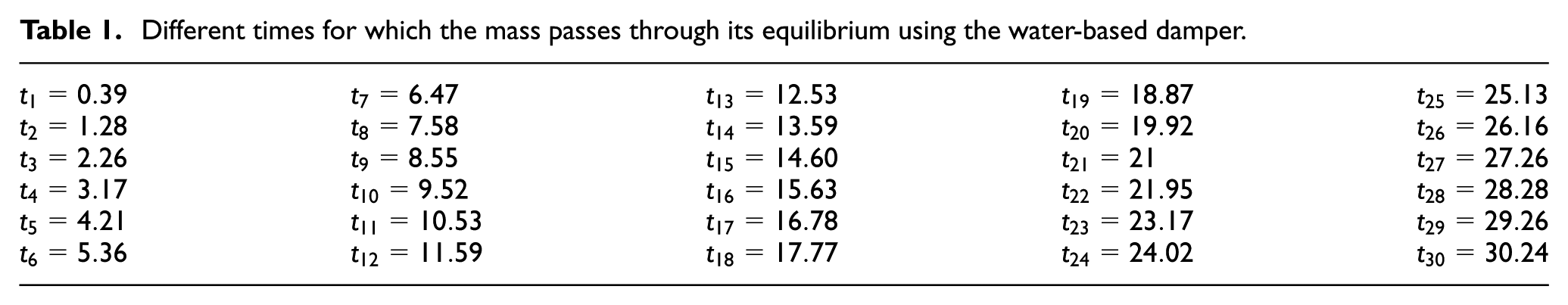
In these times, we will calculate the quasi-period τ, while the mass takes to achieve two consecutive peaks (either maximum or minimum). For this, we consider the average of the consecutive differences in the time it takes to go through its mass equilibrium point; that is to say

\frac{1}{29} \sum_{i = 1}^{29} (t_{i + 1} - t_{i}) = 1.02931034

(18)

The standard deviation of this measure is $SD = 0.08383364$ . Therefore, $τ / 2 \in [0.94547671, 1.11314398]$ . Then we consider $τ / 2 = 1.02931034$ and $τ / 4 = 0.51465517$ as the time it takes to get from the mass equilibrium point to an end point (maximum or minimum). After $t_{30}$ , the movement became indistinguishable; this is seen as the cardboard prevents the laser pass; see Figure 3. Written accurately, it must be

\forall t, t_{30} < t, | y (t) | \leq 0.005 m

(19)

with $τ / 4$ estimated λ and therefore β. Whereas $y (t)$ is the exponential curve that defines the solution of equation (17), we have $y (t) = y_{0} \cdot E_{γ} {- (β / 2 m) t_{p}^{1 - γ} t^{γ}}$ ; from the experiment, we know that $y (0) = 0.05$ and $t_{30}$ was the last time for which the mass passes through its equilibrium point before moving out indistinguishable; with these considerations, we can assume that

\begin{array}{l} y (t_{30} + \frac{τ}{4}) = y (30.24 + 0.51465517) \\ = y (30.75465517) = 0.005 \end{array}

(20)

Figure 3.

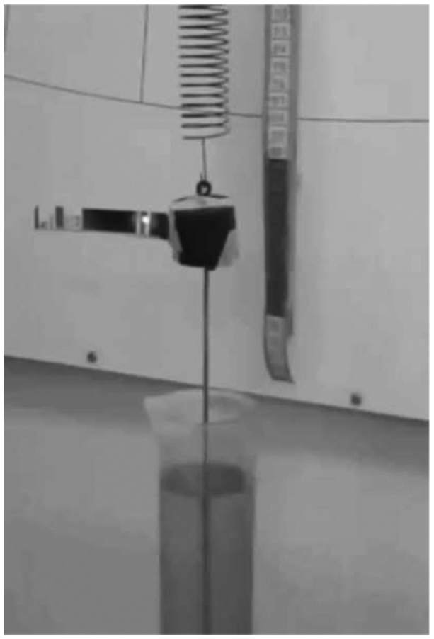
Mass–spring–viscodamper system used in this experiment.

In the fractional case, from equation (16) we have

y (t) = y_{0} \cdot E_{γ} {- \frac{β}{2 m} t_{p}^{1 - γ} t^{γ}}

(21)

where

E_{γ} (- \frac{β}{2 m} t_{p}^{1 - γ} t^{γ}) = \frac{y (t)}{y_{0}}

(22)

For obtaining β, we have

β = - (\frac{2 m}{t_{p}^{1 - γ} t^{γ}}) \cdot L_{γ} (\frac{y (t)}{y_{0}})

(23)

where $m = 0.2197 kg$ , $y (t) = 0.005$ , $y (0) = 0.05$ , β is the non-local damping coefficient, $L_{γ}$ is the inverse Mittag-Leffler function, and γ is the order of the fractional derivative.

Function Mittag-Leffler shape $E_{α, β} (- x)$ can be approximated by the Padé method defined in the range $[0, + \infty)$ as follows

Γ (β - α) x E_{α, β} (- x) \approx \frac{p (x)}{q (x)} = \frac{p_{0} + p_{1} x + \dots + p_{ν} x^{ν}}{q_{0} + q_{1} x + \dots + q_{ν} x^{ν}}

(24)

where ν is an integer. The problem is finding the coefficients $p_{i}$ and $q_{i}$ such that equation (24) be a correct expansion in $x = 0$ and $x = \infty$ .

The solution to the above equation is

E_{α, β} (- x) \approx \frac{1}{Γ (β - α)} \frac{p_{0} + p_{1} x + x^{2}}{q_{0} + q_{1} x + x^{2}} = \frac{\frac{1}{Γ (β)} + \frac{1}{Γ (β - α) q_{0}} x}{1 + \frac{q_{1}}{q_{0}} x + \frac{1}{q_{0}} x^{2}}

(25)

Hilfer and Seybold⁴⁰ studied the inverse Mittag-Leffler function $L_{α, β} (x)$ , defined as the solution of equation^41–43

L_{α, β} (E_{α, β} (x)) = x

(26)

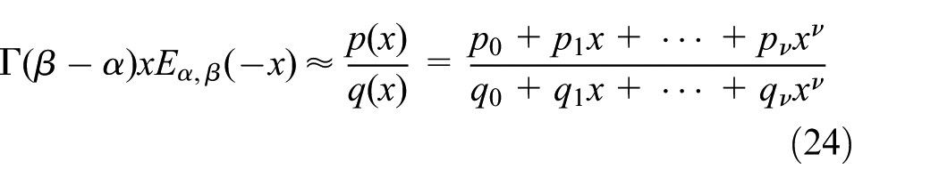
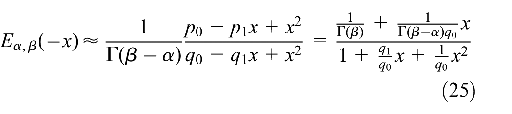
The global Padé approximation^44–46 of the generalized Mittag-Leffler function $E_{α, β} (- x)$ assesses the generalized inverse function $- L_{α, β} (x)$ . Solving the quadratic equation (25) and rearranging, we have the global Padé approximation of $- L_{α, β} (x)$ with grade 2 as

\begin{array}{l} - L_{α, β} (x) \approx \frac{1}{2 Γ (β - α)} - \frac{q_{1}}{2} \\ + \sqrt{{(\frac{q_{1}}{2} - \frac{1}{2 Γ (β - α) x})}^{2} - q_{0} (1 - \frac{1}{Γ (β) x})} \end{array}

(27)

where ${L_{α, β} (x) |}_{x \to 0^{+}} = + \infty$ and ${L_{α, β} (x) |}_{x \to \frac{1}{Γ (β)}} = 0$ .

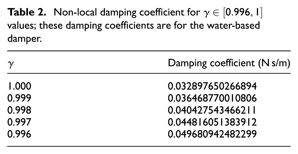
Table 2 shows the non-local damping coefficient defined by different values of γ.

Table 2.

Non-local damping coefficient for $γ \in [0.996, 1]$ values; these damping coefficients are for the water-based damper.

$γ$	Damping coefficient (N s/m)
1.000	0.032897650266894
0.999	0.036468770010806
0.998	0.040427543466211
0.997	0.044816051383912
0.996	0.049680942482299

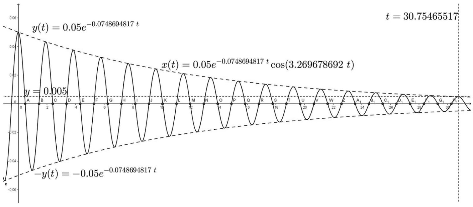
In the classical case, considering $k = 2.35 N / m$ , $m = 0.2197 kg$ , and $β = 0.032897650266894 N s / m$ , the times measured are obtained for which the mass crosses its equilibrium point; see Figure 4.

Figure 4.

Graphical displacement of $x (t)$ . The points A through $H_{1}$ correspond to times $t_{1}$ to $t_{32}$ in Table 3. Note that $x (t_{30} + τ / 4) = 0.005$ .

The graph of $x (t)$ is presented in Figure 4; this figure shows 32 courts with the horizontal axis; these values are listed in Table 3. While our experience in the laboratory with the mass–spring–viscodamper system, we studied only system that crossed 30 times; see Table 1; this is because the quasi-period used came from the average of the measurements we made during the experiment. This approach is sufficient for the purposes of this investigation.

Table 3.

Roots of $x (t)$ using the water-based damper; from $t_{1}$ to $t_{32}$ , they correspond to the points A to $H_{1}$ in Figure 4.

$t_{1} = 0.4804130596$	$t_{12} = 11.0495000950$	t ₂₃ = 21.6185873075
$t_{2} = 1.4412392082$	$t_{13} = 12.0103263559$	t ₂₄ = 22.5794134253
$t_{3} = 2.4020653868$	$t_{14} = 12.9711524644$	t ₂₅ = 23.5402394998
$t_{4} = 3.3628915810$	$t_{15} = 13.9319785728$	t ₂₆ = 24.5010655374
$t_{5} = 4.3237172738$	$t_{16} = 14.8928047281$	t ₂₇ = 25.4618920516
$t_{6} = 5.2845344590$	$t_{17} = 15.8536309531$	t ₂₈ = 26.4227180636
$t_{7} = 6.2453695770$	$t_{18} = 16.8144567021$	t ₂₉ = 27.3835441034
$t_{8} = 7.2061956466$	$t_{19} = 17.7752829600$	t ₃₀ = 28.3443702046
$t_{9} = 8.1670221348$	$t_{20} = 18.7361092120$	t ₃₁ = 29.3051963520
$t_{10} = 9.1278480236$	$t_{21} = 19.6969354444$	t ₃₂ = 30.2660225297
$t_{11} = 10.0886743314$	$t_{22} = 20.6577761145$

Figure 5(a)–(d) shows different solutions of equation (16) for the classical case $γ = 1$ and $β = 0.036468770010806 Ns / m$ , $β = 0.040427543466211 Ns / m$ , $β = 0.044816051383912 Ns / m$ , and finally when $β = 0.049680942482299 Ns / m$ , respectively.

Figure 5.

Graphical displacement of $x (t)$ with different β values, the damping coefficients corresponding to water.

Now they are going to consider the results of studying a pair of oil-based buffers, one edible (sunflower oil) and one with gasoline engine oil (SAE 10W-40). Declining oil reserves worldwide have brought to the field of research on the physical properties of vegetable oils as lubricants for being renewable and have a high rate biodegradability.⁴⁷ The times measured for edible oil damper are shown in Table 4.

Table 4.

Times when the mass passes through its equilibrium point for the shock of edible oil.

t ₁ = 0.69	t ₆ = 5.99	t ₁₁ = 11.53
t ₂ = 1.70	t ₇ = 7.09	t ₁₂ = 12.60
t ₃ = 2.73	t ₈ = 8.13	t ₁₃ = 13.68
t ₄ = 3.88	t ₉ = 9.16	t ₁₄ = 14.67
t ₅ = 4.87	t ₁₀ = 10.32	t ₁₅ = 15.90

With the times in Table 4, $τ / 2$ is determined calculating the average of the consecutive differences, as before, when the water-based damper was studied

\frac{1}{14} \sum_{i = 1}^{14} (t_{i + 1} - t_{i}) = 1.08642857

(28)

The standard deviation of this measure is $SD = 0.07840792$ . Therefore, $τ / 2 \in [1.00802065, 1.16483649]$ . Then we consider $τ / 2 = 1.08642857$ and $τ / 4 = 0.54321429$ as the approximate time it takes to go from its mass equilibrium point to immediate peak (either maximum or minimum). We shall assume, as before, that $y (t)$ function is the exponential curve that defines the solution of equation (17); we have $y (t) = y_{0} \cdot E_{γ} {- (β / 2 m) t_{p}^{1 - γ} t^{γ}}$ ; from the experiment, we know that $y (0) = 0.05$ and $t_{15}$ was the last time for which the mass passes through its equilibrium point before moving out indistinguishable; with these considerations, it can be assumed that

\begin{array}{l} y (t_{15} + \frac{τ}{4}) = y (15.90 + 0.54321429) \\ = y (16.44321429) = 0.005 \end{array}

(29)

Considering $m = 0.2197 kg$ , $y (t) = 0.005$ , and $y (0) = 0.05$ , the solutions of equation (23) are shown in Table 5. Table 5 shows the non-local damping coefficient defined by different values of γ.

Table 5.

Non-local damping coefficient for $γ \in [0.996, 1]$ values; these damping coefficients are for the buffer-based edible oil.

γ	Damping coefficient (N s/m)
1.000	0.061530298883041
0.999	0.061581751641900
0.998	0.061633474367095
0.997	0.061685468536235
0.996	0.061737735637375

In the classical case, considering $k = 2.35 N / m$ , $m = 0.2197 kg$ , and $β = 0.061530298883041 Ns / m$ , the times are obtained for which the mass crosses its equilibrium point; see Figure 6. The graph of $x (t)$ has 17 cuts with respect to the horizontal axis; these values are listed in Table 6. While our experience in the laboratory with the spring–mass–viscodamper system, we studied only system that crossed 15 times; see Table 4; this is because the quasi-period average employee came from measurements that we made during the experiment. This approach is sufficient for the purposes of this investigation.

Figure 6.

Graph of $x (t)$ displacement of the mass using the damper-based edible oil. Note that the roots numbered from A to Q shown in Table 6 are twice more observed in the experiment listed in Table 4.

Table 6.

Roots of numerical simulation for $x (t)$ solution in the case of damper-based edible oil (see Figure 6).

$t_{1} = 0.4807279951$	$t_{7} = 6.2494640294$	$t_{13} = 12.0182000384$
$t_{2} = 1.4421838833$	$t_{8} = 7.2109198694$	$t_{14} = 12.9796563551$
$t_{3} = 2.4036401999$	$t_{9} = 8.1723760703$	$t_{15} = 13.9411121495$
$t_{4} = 3.3650960145$	$t_{10} = 9.1338320225$	$t_{16} = 14.9025679857$
$t_{5} = 4.3265518089$	$t_{11} = 10.0952882451$	$t_{17} = 15.8640242104$
$t_{6} = 5.2880080653$	$t_{12} = 11.0567441269$

Figure 7(a)–(d) shows different solutions of equation (16) for the classical case $γ = 1$ and $β = 0.061581751641900 N s / m$ , $β = 0.061633474367095 N s / m$ , $β = 0.061685468536235 N s / m$ , and finally when $β = 0.061737735637375 N s / m$ , respectively.

Figure 7.

Graphical displacement of $x (t)$ with different β values, the damping coefficients corresponding to edible oil.

The times measured for which the mass passes through the equilibrium point with oil motor–based damper are shown in Table 7.

Table 7.

Times for which the mass passes through its equilibrium using the damper with motor oil.

t_{1} = 0.63

t_{2} = 1.64

t_{3} = 2.74

t_{4} = 3.88

t_{5} = 5.08

With the times in Table 7, $τ / 2$ is determined calculating the average of the consecutive differences

\frac{1}{4} \sum_{i = 1}^{4} (t_{i + 1} - t_{i}) = 1.1125

(30)

The standard deviation of this measure is $SD = 0.07973916$ . Therefore, $τ / 2 \in [1.03276084, 1.19223916]$ . Then we consider $τ / 2 = 1.1125$ and $τ / 4 = 0.55625$ as the approximate time it takes to go from its equilibrium point to immediate peak (either maximum or minimum). We shall assume, as before, that the $y (t)$ function is the exponential curve that defines the solution of equation (17); we have $y (t) = y_{0} \cdot E_{γ} {- (β / 2 m) t_{p}^{1 - γ} t^{γ}}$ ; from the experiment, we know that $y (0) = 0.05$ and $t_{5}$ was the last time for which the mass passes through its equilibrium point before moving out indistinguishable; with these considerations, it can be assumed that

y (t_{5} + \frac{τ}{4}) = y (5.08 + 0.55625) = y (5.63625) = 0.005

(31)

Considering $m = 0.2197 kg$ , $y (t) = 0.005$ , and $y (0) = 0.05$ , the solutions of equation (23) are shown in Table 8. Table 8 shows the non-local damping coefficient defined by different values of γ.

Table 8.

Non-local damping coefficient for $γ \in [0.996, 1]$ values; these damping coefficients are for the damper-based motor oil.

γ	Damping coefficient (N s/m)
1.000	0.179508696360450
0.999	0.198657428298286
0.998	0.219848813000371
0.997	0.243300746373796
0.996	0.269254367936689

In the classical case, considering $k = 2.35 N / m$ , $m = 0.2197 kg$ , and $β = 0.179508696360450 N s / m$ , the times measured for which the mass crosses its equilibrium point are obtained; see Figure 8.

Figure 8.

Graphical mass displacement of $x (t)$ using the damper-based motor oil. Zero crossings A to F correspond to the times $t_{1}$ to $t_{6}$ in Table 9.

This graph has six cuts with the horizontal axis; these values are listed in Table 9. While our experience in the laboratory with the spring–mass–viscodamper system, we studied only system that crossed five times; see Table 7; this is because the quasi-period average employee came from measurements that we made during the experiment. This approach is sufficient for the purposes of this investigation.

Table 9.

Roots of numerical simulation for $x (t)$ solution in the case of oil-based damper motor (see Figure 8).

t ₁ = 0.4840783702

t ₂ = 1.452235811

t ₃ = 2.4203929387

t ₄ = 3.3885499778

t ₅ = 4.356707158

t ₆ = 5.3248646445

Figure 9(a)–(d) shows different solutions of equation (16) for the classical case $γ = 1$ and $β = 0.198657428298286 N s / m$ , $β = 0.219848813000371 N s / m$ , $β = 0.243300746373796 N s / m$ , and finally when $β = 0.269254367936689 N s / m$ , respectively.

Figure 9.

Graphical displacement of $x (t)$ with different β values, the damping coefficients corresponding to motor oil SAE 10W-40.

Conclusion

In this work, we obtain the viscous damping coefficient β theoretically and experimentally in the spring–mass–viscodamper system. The influence of the viscosity of the fluid and the damping coefficient is analyzed using three fluids, water, edible oil, and gasoline engine oil SAE 10W-40. Applying the Caputo fractional derivative to the classical equation of harmonic oscillator equation (16), a generalized model of this oscillator is obtained; the obtained solution incorporates and describes long-term memory effects (attenuation or dissipation); these effects are related to an algebraic decay related to the Mittag-Leffler function; in this context, when γ is less than 1, the fractional differentiation with respect to the time represents a non-local displacement effect of dissipation of energy (internal friction) represented by the fractional order γ; the fractional order is related to the displacement of the oscillator in fractal geometries.

In the classic case when $γ = 1$ , the system displays the Markovian nature and damping coefficient is considered constant, which is close enough to reality to no turbulent viscous dampers. However, for values of $γ = 1$ , the equations describe systems non-conservative (non-local in time); in this context, the different γ values modified the time constant of the systems and exhibit fractional structures (components that show an intermediate behavior between a system conservative and dissipative). Applying the inverse function of Mittag-Leffler coefficient, non-local damping for different values of γ is obtained, which are reported in Tables 2, 5, and 8 for $γ \in (0.996, 1)$ . At the range $γ \in (0.996, 1)$ , the figures show that the system presents dissipative effects that correspond to the nonlinear situation of the physical process (realistic behavior that is non-local in time). In these cases, the systems modified the damping capacity, for example, when $γ = 0.996$ , the damping capacity is bigger that when $γ = 0.999$ . Due to the viscous energy dissipation, the damping coefficients may have very complex properties, for example, this damping capacity is of viscoelastic type when having both viscous and elastic characteristics that avoid or dampen oscillation-free system. The damping rate viscous-viscoelastic it occurs when at high speed the system only presents viscous friction and when at low speeds only becomes viscoelastic friction; in the opposite case, when the system acquires at high speeds only viscoelastic friction and when at low speeds only acquires viscous friction then damping coefficient is called viscoelastic-viscous.^48,49

Because some authors replace the derivative of a fractional entire order in a purely mathematical context, the physical parameters involved in the differential equation do not have the dimensionality obtained in the laboratory; from the physical point of view of engineering, this is not entirely correct; in this representation, an auxiliary parameter $σ = t_{p}$ is introduced; this parameter characterizes the existence of the fractional temporal components and relates the time constant of the system; in this context, the solutions presented here preserve the dimensionality of the studied system for any value of the exponent of the fractional derivative. The advantage of this alternative representation when compared with the models presented in the literature is the physical compatibility of the solutions.

The methodology used to approximate the value of the damping coefficient is very accurate; discrepancies between the times measured in the laboratory with the numerical solutions are due to the way in which data and the dependence of the damping coefficient with the quasi-period were taken. But laboratory tests, even with their own technical difficulties of the experiment, are sufficient to support our research in analytical terms from the perspective of FC. Since they allowed to find the solution for the fractional dynamic model where the fractional order of damping changes continuously. We consider that these results are useful to understand the behavior of dynamical complex systems, mechanical vibrations, control theory, relaxation phenomena, viscoelasticity, viscoelastic damping, and oscillatory processes.

Footnotes

Acknowledgements

The authors would like to thank Mayra Martínez for the interesting discussions.

Academic Editor: Norman Wereley

Declaration of conflicting interests

The author(s) declared the following potential conflicts of interest with respect to the research, authorship, and/or publication of this article: José Francisco Gómez Aguilar acknowledges the support provided by Cátedras CONACYT para jóvenes investigadores 2014.

Funding

The author(s) received no financial support for the research, authorship, and/or publication of this article.

References

Oldham

Spanier

The fractional calculus. New York: Academic Press, 1974.

Miller

Ross

An introduction to the fractional calculus and fractional differential equations. New York: John Wiley & Sons, 1993.

Podlubny

Fractional differential equations. San Diego, CA: Academic Press, 1999.

Baleanu

Günvenc

Tenreiro Machado

JA.

New trends in nanotechnology and fractional calculus applications. New York: Springer, 2010.

Baleanu

Fractional calculus models and numerical methods. Singapore: World Scientific Publishing Company, 2012.

Uchaikin

Fractional derivatives for physicists and engineers. New York: Springer, 2013.

Shen

Soong

TT.

Modeling of viscoelastic dampers for structural applications. J Eng Mech: ASCE 1995; 121: 694–701.

Koeller

RC.

Application of fractional calculus to the theory of viscoelasticity. J Appl Mech: T ASME 1984; 51: 299–307.

Enelund

Ahler

Runesson

. Formulation and integration of the standard linear viscoelastic solid with fractional order rate laws. Int J Solids Struct 1999; 36: 2417–2442.

10.

Ingman

Shzdalnitsky

Iteration method for equation of viscoelastic motion with fractional differential operator of damping. Comput Method Appl M 2001; 190: 5027–5036.

11.

Hilfer

Applications of fractional calculus in physics. Singapore: World Scientific Publishing Company, 2000.

12.

Kilbas

Srivastava

Trujillo

JJ.

Theory and applications of fractional differential equations. Amsterdam: Elsevier, 2006.

13.

Kiryakova

Generalized fractional calculus and applications. New York: John Wiley & Sons, 1994.

14.

Das

Functional fractional calculus. New York: Springer, 2011.

15.

Rossikhin

Shitikova

MV.

Application of fractional operators to analysis of damped vibrations of viscoelastic single-mass systems. J Sound Vib 1997; 199: 567–686.

16.

Hilfer

Experimental evidence for fractional time evolution in glass forming materials. Chem Phys 2002; 284: 399–408.

17.

Mainardi

Fractional calculus and waves in linear viscoelasticity. London: Imperial College Press, 2010.

18.

Tenreiro Machado

Galhano

AMSF

Trujillo

JJ.

On development of fractional calculus during the last fifty years. Scientometrics 2014; 98: 577–582.

19.

Gómez-Aguilar

Miranda-Hernández

López-López

. Modeling and simulation of the fractional space-time diffusion equation. Commun Nonlinear Sci 2016; 30: 115–127.

20.

Garra

Giusti

Mainardi

. Fractional relaxation with time-varying coefficient. Fract Calc Appl Anal 2014; 17: 424–439.

21.

Gómez-Aguilar

Yépez-Martínez

Escobar-Jiménez

. Universal character of the fractional space-time electromagnetic waves in dielectric media. J Electromagnet Wave 2015; 29: 727–740.

22.

Magin

RL.

Fractional calculus in bioengineering. Roddin: Begell House Publisher, 2006.

23.

Gómez Aguilar

Baleanu

. Solutions of the telegraph equations using a fractional calculus approach. Proc Rom Acad Ser A 2014; 1: 27–34.

24.

Kutay

Ozaktas

HM.

The fractional Fourier transform and harmonic oscillation. Nonlinear Dynam 2002; 29: 157–172.

25.

Ryabov

Puzenko

Damped oscillations in view of the fractional oscillator equation. Phys Rev B 2002; 66: 1–8.

26.

Caputo

The memory damped seismograph. Boll Geofis Teor Appl 2013; 54: 217–228.

27.

Stanislavsky

AA.

Fractional oscillator. Phys Rev E 2004; 70: 1–6.

28.

Naber

Linear fractionally damped oscillator. Int J Differ Equat 2010; 2010: 197020 (12 pp.).

29.

Gómez-Aguilar

Rosales-García

Bernal-Alvarado

. Fractional mechanical oscillators. Rev Mex Fís 2012; 58: 348–352.

30.

Ambrosini

Cuitiño

Rebecco

Eficiencia de amortiguadores de masa sintonizados en estructuras sismorresistentes. Mec Comput 2004; 23: 447–462.

31.

Donado

Mendoza

Valencia

. Estudio experimental de la viscosidad de un fluido magneto-reológico a base de magnetita mineral. Rev Mex Fís E 2007; 53: 31–40.

32.

Rosales

Filipich

Escalante

Dinámica de una estructura flotante amarrada: modelado de la nolinealidad mediante recurrencias algebraicas. Mec Comput 2003; 22: 1051–1063.

33.

Seixas

Melcio

Mendes

VMF

. Offshore wind turbine simulation: multibody drive train. Back-to-back NPC (neutral point clamped) converters. Fractional-order control. Energy 2014; 69: 357–369.

34.

Brommundt

Muskulus

Strach

. Experiences with object-oriented and equation based modeling of a floating support structure for wind turbines in Modelica. In: Proceedings of the 2012 winter simulation conference (WSC), Berlin, 9–12 December 2012, vol. 1, pp. 1–12. New York: IEEE.

35.

Zhu

Cai

Spanos

PD.

A nonlinear and fractional derivate viscoelastic model for rail pads in the dynamic analysis of coupled vehicle-slab track systems. J Sound Vib 2015; 335: 304–320.

36.

Haubold

Mathai

Saxena

RK.

Mittag-Leffler functions and their applications. J Appl Math 2011; 1: 1–51.

37.

Gómez-Aguilar

Escobar-Jiménez

Olivares-Peregrino

. Nonlocal electrical diffusion equation. Int J Mod Phys C 2016; 27: 1–12.

38.

Gómez Aguilar

Baleanu

. Fractional transmission line with losses. Z Naturforsch 2014; 69: 539–546.

39.

Ertik

Çalik

Sirin

. Investigation of electrical RC circuit within the framework of fractional calculus. Rev Mex Fis 2015; 61: 58–63.

40.

Hilfer

Seybold

Computation of the generalized Mittag-Leffler function and its inverse in the complex plane. Integr Transf Spec F 2006; 17: 637–652.

41.

Seybold

Hilfer

Numerical algorithm for calculating the generalized Mittag-Leffler function. Siam J Numer Anal 2008; 47: 69–88.

42.

Gorenflo

Loutchko

Luchko

Computation of the Mittag-Leffler function E_a,b(z) and its derivatives. Fract Calc Appl Anal 2002; 5: 491–518.

43.

Hanneken

Narahari

ABN

. Finite series representation of the inverse Mittag-Leffler function. Math Probl Eng 2014; 1: 1–18.

44.

Atkinson

Osseiran

Rational solutions for the time-fractional diffusion equation. SIAM Appl Math 2011; 71: 92–106.

45.

Mainardi

. On some properties of the Mittag-Leffler function E_α(−t^α), completely monotone for t > 0 with 0 < α < 1, 2013, http://arxiv.org/abs/1305.0161

46.

Garrappa

Popolizio

Evaluation of generalized Mittag-Leffler functions on the real line. Adv Comput Math 2013; 39: 205–225.

47.

Rodrguez-Martnez

Lafargue-Pérez

Sotolongo-Pérez

. Determinación de las propiedades fsicas y carga crtica del aceite vegetal jatropha curcas l. Ing Mec 2012; 15: 170–175.

48.

Eslahchi

Dehghan

Parvizi

Application of the collocation method for solving nonlinear fractional integro-differential equations. J Comput Appl Math 2014; 257: 105–128.

49.

Lakes

RS.

Viscoelastic materials. Cambridge: Cambridge University Press, 2009.

Experimental evaluation of viscous damping coefficient in the fractional underdamped oscillator

Abstract

Keywords

Introduction

Basic tools

The fractional damping model

Experimental setup

Conclusion

Footnotes

Acknowledgements

Declaration of conflicting interests

Funding

References