On finding exact and approximate solutions to fractional systems of ordinary differential equations using fractional natural adomian decomposition method
Open accessResearch articleFirst published online 2022
On finding exact and approximate solutions to fractional systems of ordinary differential equations using fractional natural adomian decomposition method
In this work, we present proofs for new theorems that deal with natural transform method (NTM) with Caputo derivative. Also, we give exact and approximate solutions to systems of fractional differential equations along with fractional ordinary and partial differential equations using the fractional natural decomposition method (FNDM). The Caputo derivative is used here to minimize the amount of computational, and this is of great significance for large-scale problems. The work outlines the significant features of the FNDM. Our work can be considered as another technique to existing methods, and will have many applications in variant areas of science and engineering.
Fractional derivatives have proven their capability to describe several phenomena associated with memory and aftereffects due to their non-locality property.1 Such phenomena are commonplace in physical processes, biological structures, and cosmological phenomena. For instance, the fractional Kelvin-Voigt rheological models have been employed to examine the low applied force frequencies.2–5 For this reason, this became necessary to illuminate the solutions of the models that describe these phenomena. Several analytical techniques were presented to achieve their objectives. Actually, all these approaches were accommodation for the existing methods to handle the integer case models which is natural since the fractional derivative generalizes the classical derivative to an arbitrary order.
Recently, fractional calculus and their applications have been treated by many researchers, see4–9 and the references therein. Even though fractional derivatives have existed as long as their integer order counterparts, but only in recent decades have fractional derivative models became exciting new tools in the study of practical problems in disciplines as diverse as physics,10–12 finance,13,10 biology5,6 and hydrology.3,14,9,15 As fractional derivative models are becoming increasingly popular among the wider scientific community, is the main motivation to study numerical schemes for fractional differential equations. There are many applications of fractional differential equations and just to name few: control systems, elasticity, electric drives, circuits systems, continuum mechanics, heat transfer, quantum mechanics, fluid mechanics, signal analysis, biomathematics, biomedicine, social systems and bio-engineering.
Lately, many techniques discussed the way how to explore approximate solutions of FDEs, such as FDTM,16 the fractional sub-equation method,9 the FNDM,11,12,17,18 the FVM,4 the modified homotopy perturbation method (MHPM),19 the Conformable Sumudu Decomposition Method20 and the (FADM).21,15 The outline of our work is as follows: First, in Chapters 2, we give the history of natural transform method, definitions of fractional derivatives. In chapter 3, we present proofs to theorems related to the natural fractional derivatives. Chapter 4 is devoted for applications model of FDEs using the proposed method. In chapter 5, we solve fractional systems of ODEs. Finally, our concluding remarks is presented, in chapter 6, to outline of what we have accomplished in this research.
Related Materials
We explore some definitions terminologies of natural transform that will be needed later on in the proofs of our results, (see for example,22,13,10).
We say a function , where , if with , such that , and , and we say , if where .
If . We define the Caputo type of as
23 The Mittag-Leffler in two parameters is given by
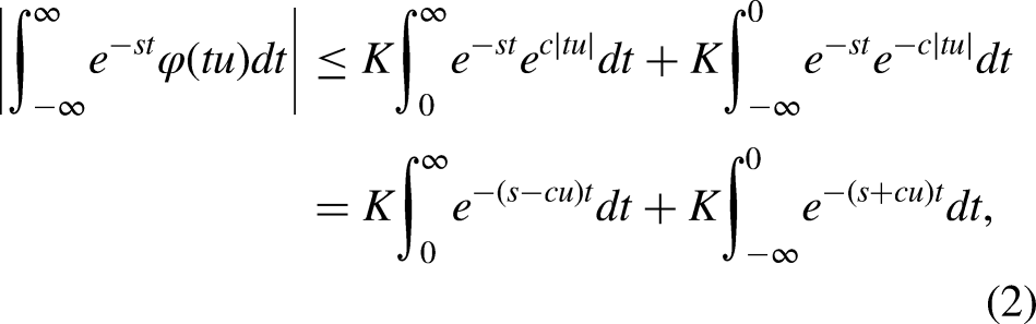
Let denote the Heaviside function, more precisely for and for . We introduce a real-valued function, on which -transform can be defined on [0, ), where , . Let be continuous on . For some . Consider
Note that for any in the class we have
which is convergent provided that . Then, we define the natural transform
Alternatively,
Note that one can obtain the Laplace transform and the Sumudu transform if we plug in , in the above equations, respectively.
We shall use the well-known gamma function through out this paper
where .
Important Properties
Some basic properties of the N-transforms are given as follows22,11,12
.
Natural Caputo Fractional Derivatives
Here we give detailed proofs to some theorems of N-transform of Caputo fractional derivative. The proofs of theorem (1) was given in another published paper by the first author.
Caputo Fractional Derivative
For the sake of readers, we give just some of natural transforms properties. We direct the reader for more properties to see for example.22,11,12
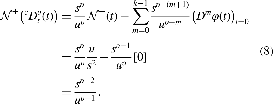
If , where . Then, the N-transform of Caputo derivative of is
The natural transform of the Caputo derivative for is given by
The natural transform of the Caputo derivative for is
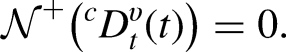
First note that . Then, we get
The proof of Theorem (5) is complete. □
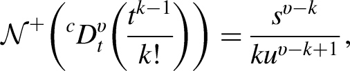
The Caputo Fractional Natural Transform of is
First note that
The proof of Theorem (6) is complete. □
Applications of FNDM for Fractional ODEs and PDEs
For this section, we shall implement the new scheme to solve two nonlinear fractional ODEs and we present solution to the diffusion fractional differential equations. Finally, we present numerical tables for these examples for multiple values of and .
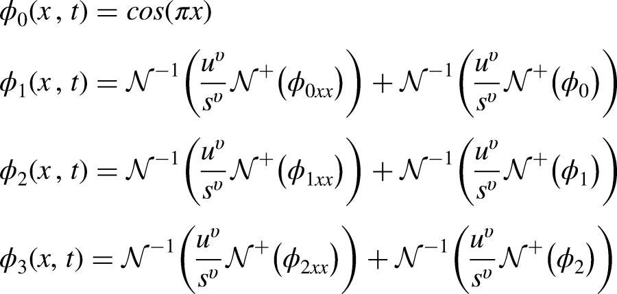
Methodology of FDM
Consider the general nonlinear (FODE)
where and , and along with initial condition
where is the Caputo derivative for , is the linear differential operator and represents the nonlinear part. Also is the non-homogeneous part.
This is indeed the intended solution for equation (29) which exists through out the literature (Figures 2 and 3).
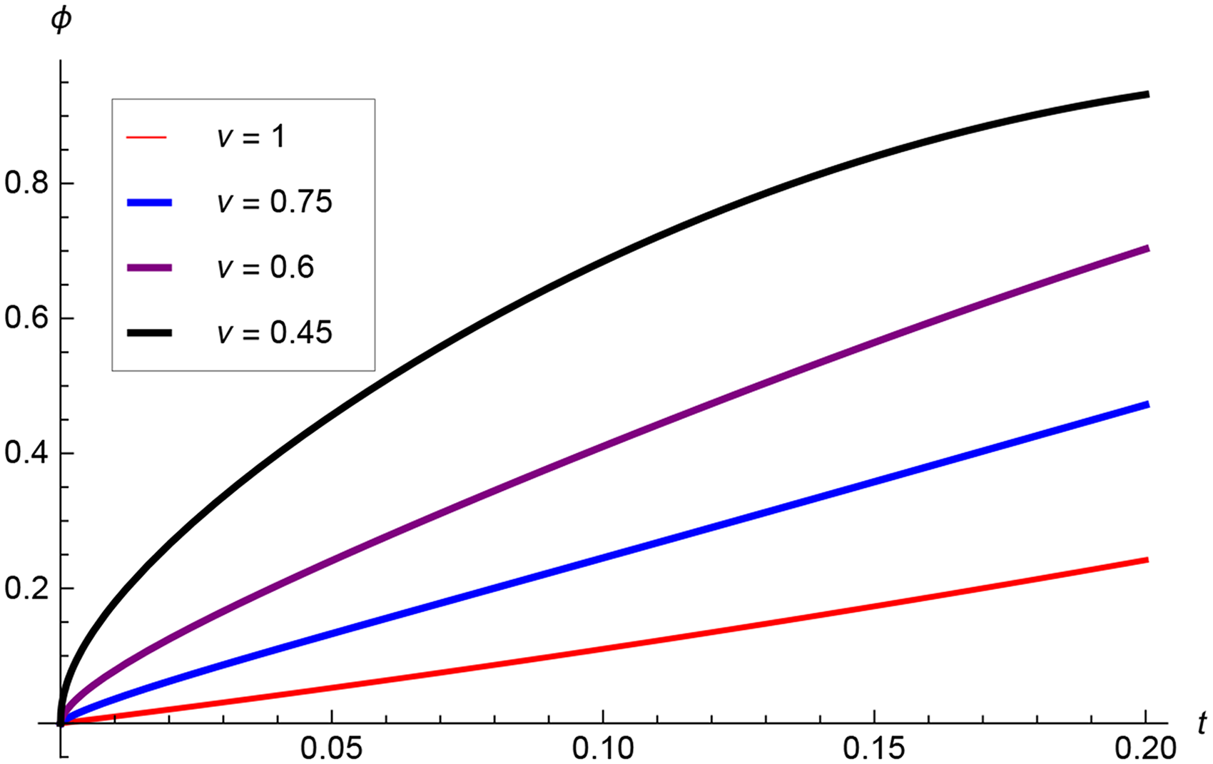
Exact solutions for example 4.2 with , respectively.
Exact solutions for example 4.2 with , respectively.
Remark.Figure 2 shows that the solution peak is high and one can see that the peak of the solutions of the diffusion equation becomes more and more smooth as the fractional factor increases (Table 2).
Numerical results for Example 2 for distinct values for .
x
t
Numerical
Exact
0
0.02
0.20104552
0.36691625
0.61998793
0.83745132
0.83745132
0.04
0.17414299
0.28187077
0.46534302
0.70132479
0.70132479
0.06
0.15978832
0.23813296
0.37076063
0.58732540
0.58732540
0.08
0.1502041
0.21016121
0.30658126
0.49185646
0.49185646
0.1
0.14310464
0.19025412
0.26034611
0.41190586
0.41190586
1/4
0.02
0.14216065
0.25944897
0.43839767
0.59216754
0.59216754
0.04
0.12313769
0.19931273
0.32904721
0.49591151
0.49591151
0.06
0.11298741
0.16838543
0.26216736
0.41530177
0.41530177
0.08
0.10621033
0.14860641
0.21678569
0.34779504
0.34779504
0.1
0.10119026
0.13452998
0.1840925
0.29126143
0.29126143
1/3
0.02
0.10052276
0.18345812
0.30999396
0.41872568
0.41872568
0.04
0.087071497
0.14093539
0.23267151
0.35066239
0.35066239
0.06
0.079894162
0.11906648
0.18538032
0.29366270
0.29366270
0.08
0.075102048
0.1050806
0.15329063
0.24592823
0.24592823
0.1
0.071552321
0.09512706
0.13017306
0.20595293
0.20595293
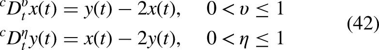
Fractional Systems of Ordinary Differential Equations
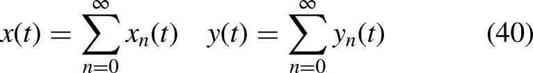
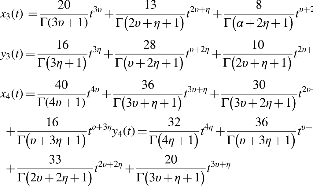
Now let us examine two models of systems of FDEs. Then, we present numerical values in tables for some values of . We only used 5 order approximate solutions for the two functions.
Finally, the approximate solutions for these functions are as follows:
It follows that,
Note that when , then the exact solutions are .
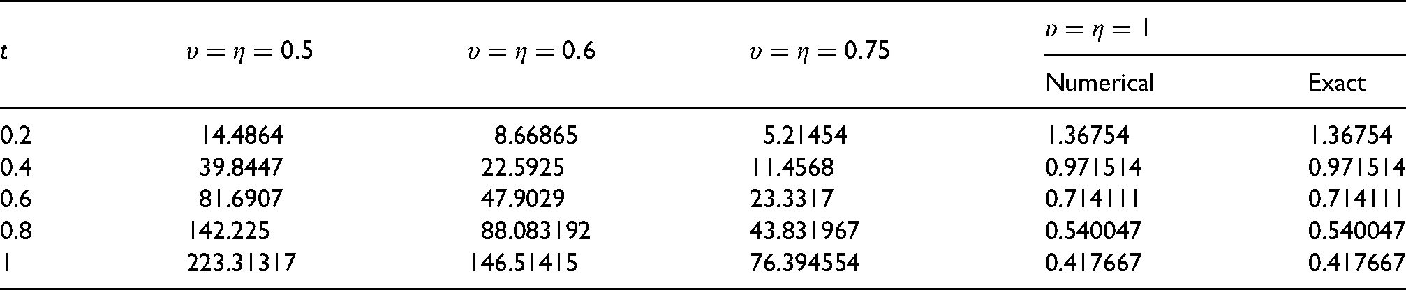
Approximate solutions for example 2 with some values of , respectively.
The results obtained for with different values of and
Numerical
Exact
0.2
14.4864
8.66865
5.21454
1.36754
1.36754
0.4
39.8447
22.5925
11.4568
0.971514
0.971514
0.6
81.6907
47.9029
23.3317
0.714111
0.714111
0.8
142.225
88.083192
43.831967
0.540047
0.540047
1
223.31317
146.51415
76.394554
0.417667
0.417667
Conclusion
Prior to this work, many techniques were used to handle FDEs. We successfully explore solutions for both linear and nonlinear ordinary FDEs and systems of FDODEs using the FNDM. We found exact and approximate solutions to systems of ordinary fractional differential equations and fractional diffusion differential equations such as diffusion model using fractional natural decomposition method (FNDM). The results showed that the new scheme is accurate and efficient. We were being able to explore solutions to physical models when . The next step for our research is to further apply the new scheme to other FDEs that arises in other areas of scientific fields.
Footnotes
Acknowledgements
We are thankful to the referees for their comments and remarks that will help in improving the quality of our work.
Funding
Funding not applicable.
Competing interests
The authors declare that they have no competing interests.
Authors contributions
All authors contributed equally to the manuscript. All authors read and approved the final manuscript.
Availability of data and materials
Data sharing not applicable to this article as no data sets were generated or analyzed during the current study.
ORCID iD
Mahmoud S. Alrawashdeh
References
1.
DuMWangZHuH. Measuring memory with the order of fractional derivative. Sci Rep2013; 3: 3431.
2.
NigmatullinRR. To the theoretical explanation of the “universal response”. Phys Stat Solidi B1984; 123(2): 739–745.
3.
CoussotCKalyanamSYappRet al. Fractional derivative models for ultrasonic characterization of polymer and breast tissue viscoelasticity. IEEE Trans Ultrason Ferroelectr., req Control2009; 56(4): 715–725.
4.
SongDYJiangTQ. Study on the constitutive equation with fractional derivative for the viscoelastic fluids-modified jeffreys model and its application. Rheol Acta1998; 37(5): 512–517.
5.
DjordjevicVDJaricJFabryBet al. Fractional derivatives embody essential features of cell rheological behavior. Ann Biomed Eng2003; 31(6): 692–699.
6.
EringenACEdelenDG. On nonlocal elasticity. Int J Eng Sci1972; 10(3): 233–248.
7.
AdomianG. A new approach to nonlinear partial differential equations. J Math Anal Appl1984; 102: 420–434.
8.
GhoshUSarkarSDasS. Solution of system of linear fractional differential equations with modified derivative of Jumarie type.” arXiv preprint arXiv:1510.00385, 2015.
9.
GuoSMeiLLiYet al. The improved fractional sub-equation method and its applications to the space–time fractional differential equations in fluid mechanics. Phys Lett A2012; 376: 407–411.
RawashdehMS. The fractional natural decomposition method: Theories and applications. Math Methods Appl Sci2017; 40(7): 2362–2376.
12.
RawashdehMSHadeelA-J. Numerical solutions for systems of nonlinear fractional ordinary differential equations using the FNDM. Mediterranean Journal of Mathematics2016; 13(6): 4661–4677.
13.
OldmanKBSpanierJ. The Fractional Calculus. New York: Academic Press, 1974.
14.
BaleanuDJassimHKAl QurashiM. Solving helmholtz equation with local fractional derivative operators. Fractal and Fractional2019; 3(3): 43.
15.
HuaYLuoaYLuZ. Analytical solution of the linear fractional differential equation by adomian decomposition method. J Comput Appl Math2008; 215: 220–229.
16.
RawashdehM. A new approach to solve the fractional harry dym equation using the FRDTM. Int J Pure Appl Math2014; 95(4): 553–566.
17.
LiZBHeJH. Fractional complex transform for fractional differential equations. Math Comput Appl2010; 15: 970–973.
18.
AlrawashdehMSBani-IssaS. An efficient technique to solve coupled–time fractional boussinesq–burger equation using fractional decomposition method. Advances in Mechanical Engineering2021 Jun; 13(6): 16878140211025424.
19.
BaleanuDJassimHK. Exact solution of two-dimensional fractional partial differential equations. Fractal and Fractional2020; 4(2): 21.
20.
ObeidatNABentilDE. New theories and applications of tempered fractional differential equations. Nonlinear Dyn2021; 105(2): 1689–1702.
21.
MomaniSShawagfehN. Decomposition method for solving fractional riccati differential equations. Appl Math Comput2006; 182(2): 1083–1092.
22.
BelgacemFBMSilambarasanR. Maxwell’s equations solutions through the natural transform. 2012; 3(3): 313–323.
23.
Mittag-LefflerGM. Sur la nouvelle fonction . C R Acad Sci Paris1903; 137: 554–558.