Sage Journals: Discover world-class research

Abstract

Methods for solving differential equations based on neural networks have been widely proposed in recent years. However, limited open literature to date has reported the choice of loss functions and the hyperparameters of the network and how it influences the quality of numerical solutions. In the present work we intend to address this issue. Precisely we will focus on possible choices of loss functions and compare their efficiency in solving differential equations through a series of numerical experiments. In particular, a comparative investigation is performed between the natural neural networks and Ritz neural networks, with and without penalty for the boundary conditions. The sensitivity on the accuracy of the neural networks with respect to the size of training set, the number of nodes, and the penalty parameter is also studied. In order to better understand the training behavior of the proposed neural networks, we further investigate the approximation properties of the neural networks in function fitting. A particular attention is paid to approximating Müntz polynomials by neural networks.

Keywords

Neural networks differential equations loss function parameter sensitivity

Introduction

Differential equations have received enormous attention for hundreds of years because of their applications in describing various phenomena and processes. For some differential equations, of classical types in particular, there exist explicit expressions for their exact solutions.¹ On the other side, a huge body of literature has been devoted to studying their numerical solutions, it is impossible to give even a very brief review here. Nevertheless, we refer to^2–4 for a review on some classical numerical methods, such as finite difference, finite element, and spectral methods, frequently used for numerically solving differential equations.

However there is still a need to develop more efficient and universal methods to solve differential equations. With the emergence of computer science and scientific computing, artificial neural networks (ANN for short) is considered as one of such methods. Algorithms based on ANN have been extensively proposed since Lee & Kang’s pioneer work on neural network algorithms for solving first-order ordinary differential equations.⁵ Later on Meade & Fernandez introduced an algorithm^6–8 based on feedforward neural networks for solving ordinary differential equations. Subsequently, Lagaris et al. proposed algorithms for solving partial differential equations on regular and irregular domains.^9,10 The key idea of their algorithm is to use the output of a single-layer neural network to construct numerical solutions that satisfy the exact boundary conditions. Based on the same idea, Mall & Chakraverty introduced a Legendre neural network¹¹ to solve ordinary differential equations. Some related works include the ANN by Pakdaman et al. proposed for solving fractional differential equations¹², and Deep Galerkin Method by Sirignano & Spiliopoulos¹³ for high-dimensional PDEs. A number of parabolic equations were used to demonstrate the efficiency of their method. E & Yu¹⁴ proposed a deep neural network method, which consists in minimizing the Ritz functional associated to the underlying boundary value problems. They termed their approach as Deep Ritz Method. Recently, Piscopo et al. applied a neural network method to the calculation of cosmological phase transitions. Michoski et al.¹⁵ investigated deep networks for compressible Euler equations, and compared the ANN to conventional finite element and finite volume methods.

For decades, ANN has been used as black boxes with a lack of theoretical understanding. Although it is an effective method for solving a wide range of problems, there has been no breakthrough in related theoretical research. To have an idea about how error analysis is possible, let’s take the example of elliptic equations. For some classical methods, such as finite element or spectral methods formulated in the Galerkin framework, the numerical solution is indeed the minimizer of the associated energy functional, and the error of the numerical solution can be bounded above by the best approximation of the exact solution in the polynomial or piecewise-polynomial space. In ANN, if the problem is formulated as the same minimization problem, that means one seeks the best approximation among all neural network functions. Therefore in principle the error of the ANN solution depends on how good the network approximates the exact solution. However one of main obstacles in ANN comes from the fact that the energy functional or other commonly used loss functions are rarely convex with respect to the hyperparameters. Thus the minimizer may never be attained. As a consequence the best approximation of the network functions tells not much about the quality of actual ANN solution. Glorot & Bengio¹⁶ showed that standard gradient descent from random initialization converges poorly with deep neural networks. They also investigated the influence of the non-linear activation functions, and proposed an initialization scheme leading to faster convergence. On the other side, there exist approximation results on neural network functions. The first contribution at this direction can be traced back to the late 80’s when Cybenko proved that a single hidden layer network can approximate any function with arbitrary errors.¹⁷ In the following years, some analysis of the function approximation using single hidden layer networks have been carried out successively; see, e.g.,^12,18–22 However, few studies have focused on the choice of the hyperparameters of the network and how it influences the numerical solution of differential equations. Nevertheless we notice the work by Shen et al.,²³ who have studied deep network approximation, characterized by the number of neurons.

To summarize, the weaknesses of the ANN in solving differential equations include: (i) loss functions are generally non-convex with respect to the hyperparameters. (ii) lack of theoretical convergence guarantees for the non-convex residual minimization. (iii) lack of efficient tool for the error analysis of ANN-based approaches for differential equations.

The aim of the present paper is to address some of these weaknesses, and intend to get a better understanding on some points. Precisely, we will first discuss possible choices of the objective functionals to be minimized in ANN for solving differential equations. Then we investigate the convergence behavior for different choices of objective functions, and how does the accuracy depend on the chosen network architecture. Finally we study the parameter sensitivity of ANN and how the hyperparameters have impact on the solution accuracy and algorithm efficiency.

The paper is organized as follows: In the next section we discuss the possible choice of the objective functionals and neural network approaches to be used in solving differential equations. Then presents numerical tests to demonstrate how the ANN solution behaves for different choices of loss functions. The treatment of the boundary condition is also discussed. In the subsequent section a series of numerical experiments will be conducted to study the effect of the parameters on the accuracy, including number of training points, number of hidden layer nodes, penalty parameter, etc. The penultimate section is devoted to studying the approximation behavior of ANN methods to target functions, and characterizing the training process in approximating specific functions. Finally, we give some concluding remarks in the final section.

Artificial neural networks and choices of loss function

This section is devoted to discuss about the possible ways to find an approximation solution to differential equations and attempts to provide some choices for loss functions in which ANN solutions can be obtained. First we regard neural networks as functions to fit exact solutions of differential equations. Notice that ANN are well suited to solving optimization problems, and a wide class of differential equations can be cast as an optimization task. Considering an ANN of a single hidden layer, that means we look for solution under the form

φ_{p} (x) : = u (x, a, W, b) = a^{T} σ (W x + b)

where

x \in R^{n}, a \in R^{H}, b \in R^{H}

and

W \in R^{H \times n}

are parameters and p represents the set of

a, W, b

. Hereafter, we use boldface letters to denote vectors or vector functions, and capital letters to mean matrices. Our task is to find these parameters to form the numerical solution

φ_{p} (x)

that is close enough to the exact solution. If we take the activation function as

σ (x) = \frac{1}{1 + e^{- x}}

, then the ANN function of single layer networks reads:

φ_{p} (x) = \sum_{i = 1}^{H} \frac{a_{i}}{1 + e^{- (w_{i} \cdot x + b_{i})}}, w_{i} \in R^{n}, a_{i}, b_{i} \in R

(1)

In the following subsections, we will explain the specific steps of solving differential equations by this method and how to construct the loss function.

Conventional numerical methods

Consider the general form of differential equations:

{\begin{array}{l} L u (x) = f (x), x \in Ω, \\ B u (x) = g (x), x \in \partial Ω, \end{array}

(2)

where

L

is a differential operator,

B

is a boundary operator,

u (x)

is the exact solution to be approximated,

x \in R^{n}

is the independent variable over the domain

Ω \subset R^{n}

, f is a given function, g is the boundary condition. If

L

is an elliptic operator, then we can find a suitable function space V and bilinear form

a (\cdot, \cdot)

such that

a (u, v) = (L u, v), \forall u, v \in V .

In many cases, the problem (2) is equivalent to the following variational problem: find $u \in V$ , such that

a (u, v) = F (v), \forall v \in V,

(3)

where

F (\cdot)

belongs to the dual space of V, which incorporates the source function f and a part of the boundary conditions (Neumann condition for example). Furthermore, if

a (\cdot, \cdot)

is coercive and symmetric, then (3) is equivalent to: find

u \in V

, such that

J (u) = \min_{v \in V} J (v),

(4)

where

J (v) = \frac{1}{2} a (v, v) - F (v) .

(5)

The problem turns out to be finding the function in the admissible function space V so that it minimizes the functional $J (\cdot)$ . Some of conventional numerical methods consist in seeking a function, i.e., approximation solution u_h, in suitable subspaces of V, say V_h, such that

a (u_{h}, v_{h}) = F (v_{h}), \forall v_{h} \in V_{h} .

(6)

Or equivalently, if $a (\cdot, \cdot)$ is coercive and symmetric: find $u_{h} \in V_{h}$ , such that

J (u_{h}) = \min_{v_{h} \in V_{h}} J (v_{h}) .

(7)

The choice of V_h distinguishes one method from another. For example, the spectral method or finite element method takes V_h as polynomial or piecewise polynomial space, while the wavelet method makes use of the space spanned by the so-called Wavelets functions.

Another way to construct numerical solutions is the so-called collocation method. To explain the idea, let’s consider the polynomial space, where the collocation approach is by far more successful than any other one. The spectral collocation solution is a polynomial u_N of degree N that satisfies

{\begin{array}{l} L u_{N} (x_{i}) = f (x_{i}), x_{i} \in Ω, \\ B u_{N} (x_{i}) = g (x_{i}), x_{i} \in \partial Ω, \end{array}

(8)

where

x_{i}

is a set of collocation points in

\bar{Ω}

. The number of the points is usually equal to the degree of freedom of the approximation solution u_N. Generally speaking, there is no available tool for numerical analysis of the collocation method, with rare exception if the collocation points are carefully selected. One of the few exceptions is the case that

x_{i}

are the Gauss-Lobatto points in a tensorial domain. In this case the collocation method for some kind of differential operators

L

can be equivalently rewritten as a variational formulation, so that an error analysis becomes possible.^2,24,25

Natural ANN method

As we have seen in the collocation method, to obtain a numerical solution for (2), we first need is to decide how to represent the solution, and then how to determine the solution. A natural idea is to take some points ${x_{i}}$ in the domain, and ask the solution to satisfy the original equation at these discrete points, or, if it is not possible, to satisfy the original equation as good as possible at these points. In collocation methods, these points are termed as collocation points, and the polynomial or piecewise polynomial is used to represent the solution. In the common practice of ANN, the discrete points are called training points, and a combination of activation functions is used as the approximation solution.

In commonly proposed ANN methods for differential equations, the numerical solution is constructed under the form

u_{p} (x) = \hat{u} (x) + b (x) φ_{p} (x),

(9)

where

φ_{p} (x)

is defined in (1),

b (x)

is chosen so as

B b (x) = 0

for all

x \in \partial Ω

and

\hat{u} (x)

exactly satisfies the boundary condition

B \hat{u} (x) = g (x), \forall x \in \partial Ω

. The advantage of this framework is that the seeked solution

u_{p} (x)

satisfies the boundary condition exactly. The task is then reduced to adjust the parameters p so that it satisfies the equation as best as possible. This can be done by, for example, minimizing the loss function:

J (p) = \frac{1}{N} \sum_{i = 1}^{N} (L u_{p} (x_{i}) - f (x_{i}))^{2},

(10)

where N is the number of training points. We will term hereafter this method as ANN with exact boundary conditions (ANN with exact BC for short).

To illustrate this method, we consider the following problem:

{\begin{array}{l} - Δ u (x, y) = f (x, y), (x, y) \in {(0, 1)}^{2}, \\ u (0, y) = u (1, y) = 0, y \in [0, 1], \\ u (x, 0) = 0, u (x, 1) = \sin (π x), x \in [0, 1] . \end{array}

Then the ANN solution can take the form

u_{p} (x, y) = y \sin π x + x (x - 1) y (y - 1) φ_{p} (x, y) .

Obviously the choice is not unique. One usually chooses the form that is easier to perform the derivatives. The drawback of the method lies in the fact that it is not always possible to find simple function satisfying the exact boundary condition, especially for complex domains.

To avoid the difficulty in constructing the boundary function, we may consider to relax the exact boundary condition by treating it as a penalty term in the loss function. That is, instead of minimizing the loss function (10), we look for a solution of form $φ_{p} (x)$ which minimizes the loss function defined by

\begin{array}{l} J (p) = \frac{1}{N} \sum_{i = 1}^{N} {(L φ_{p} (x_{i}) - f (x_{i}))}^{2} \\ + β \sum_{x_{i} \in \partial Ω} {(B φ_{p} (x_{i}) - g (x_{i}))}^{2} \end{array}

(11)

where β is a penalty parameter. Hereafter we call this method the ANN with penalty.

For both loss functions, (10) and (11), the ANN solution will be obtained by finding $p^{*}$ such that

J (p^{*}) = \min_{p} J (p) .

The superiority of the penalty method (11) over the ANN with exact BC (10) is that it is more universal, and can be easily used for any type of boundary condition. Apart from the different features of these two methods emphasized above, another interesting and important issue is about their performance, which, as far as we know, has not yet been addressed in the literature. One of the purpose of the present paper is to carry out numerical experiments to compare the performance of these two methods in term of the accuracy and convergence.

Ritz ANN method

The Ritz ANN method for differential equations was inspired by the observation that ANN is well suited for solving optimization problems, and many of differential equations can be formulated as optimization problems.

Supposing we are solving the equation (2). As we have pointed out in subsection ‘Conventional numerical methods’ , in some cases (2) can be reformulated as a minimization problem (4). Contrastly to the conventional methods which consist in finding the approximative solution in polynomial or piecewise polynomial space, the Ritz ANN method aims at seeking a function $u_{p} (x) \in V$ based on (1) such that it minimizes the functional $J (\cdot)$ defined in (5). Precisely, the Ritz ANN method is to find $p^{*}$ , such that

J (p^{*}) = \min_{p} J (p),

where

J (p) = \frac{1}{2} a (u_{p}, u_{p}) - F (u_{p})

(12)

with u_p being admissible function in V constructed based on (1) such that the essential boundary condition is satisfied. This formulation will be termed as Ritz-ANN with exact BC hereafter.

If we don’t want to have trouble with constructing admissible function in V, we can choose to relax the essential boundary condition by treating it as a penalty term in the loss function. In this case we seek the solution $φ_{p}^{*} (x)$ of the form (1) such that it minimizes the functional defined by

\begin{array}{l} J (φ_{p}) : = \frac{1}{2} a (φ_{p}, φ_{p}) - F (φ_{p}) + β \sum_{x \in \partial Ω_{e}} {(B φ_{p} (x) - g (x))}^{2}, \end{array}

(13)

where

\partial Ω_{e}

is the essential boundary. This will be called Ritz-ANN with penalty.

In actual calculations, it may be difficult to accurately calculate the integral, especially in high-dimensional space. Therefore some kind of numerical integral becomes indispensable. In our numerical experiments carried out later we will use Monte Carlo integral approximation as follows:

\int_{Ω} v (x) d x \approx | Ω | \frac{1}{N} \sum_{i = 1}^{N} v (x_{i}),

where

{x_{i}}

are the training points we take from the domain Ω.

It now remains to compute the gradient of the loss functions, which can be (10), (11), (12), or (13). This is necessary if we want to use the gradient method to solve the minimization problems. Consider an ANN with n input units, one hidden layer with H sigmoid units and one output unit. For a given input vector $x = (x_{1}, \dots, x_{n})$ , let w_ij denotes the weight from the input unit j to the hidden unit i, a_i denotes the weight of hidden unit i, and σ_i denotes the output of hidden unit i after transformed by the activation function. Then we have:

\frac{\partial^{k} φ_{p} (x)}{\partial x_{j}^{k}} = \sum_{i = 1}^{H} a_{i} w_{i j}^{k} σ_{i}^{(k)}, j = 1, 2, \dots, n,

where

σ^{(k)}

denotes the k-th order derivative of the function σ. If we take

σ (x) = \frac{1}{1 + e^{- x}}

, then

σ^{(1)} = σ (1 - σ), σ^{(2)} = σ (1 - σ) (1 - 2 σ)

, etc.

With the help of the above formulas, we can give the expression of each term of the loss function. To minimize the loss function $J (p)$ , we will use the “AdamOptimizer” module in the Tensorflow, whose mathematical principle is similar to the Newton gradient descent method. That is, the value of each parameter in the neural network during each iteration is updated in the following way:

\begin{array}{l} w_{i j} \leftarrow w_{i j} - η_{1} \frac{\partial J}{\partial w_{i j}}, \\ a_{j} \leftarrow a_{j} - η_{2} \frac{\partial J}{\partial a_{j}}, \\ b_{j} \leftarrow b_{j} - η_{3} \frac{\partial J}{\partial b_{j}}, \end{array}

where η_i are the step sizes.

In practice, there are many factors that affect the efficiency of optimizing the loss function, such as the structure of the ANN, the structure of the loss function, the value of learning rate, and so on. We will study these in depth in subsequent sections.

Comparative investigation among conventional, natural, and Ritz ANN methods

In this section, we carry out a series of numerical tests to compare the accuracy and convergence behavior between the conventional method and ANN method, and investigate the impact of different forms of loss functions on the performance of ANN method. We will give three differential equations as examples to figure how different loss functions can influence the accuracy of the numerical solutions. To ensure that the numerical solutions obtained by different loss functions are comparable, our ANN only has one hidden layer, and its nodes will be fixed. The minimization algorithm used in our numerical experiments that follow below is the AdamOptimizer module in TensorFlow.

Example 1 Consider:

{\begin{array}{l} - u ″ (x) - \frac{π^{2}}{4} u (x) = 0, x \in [0, 1], \\ u (0) = 0, u (1) = 1. \end{array}

The exact solution is $u (x) = \sin \frac{π x}{2}$

This is a classical elliptic problem, which can be reformulated into an equivalent symmetric variational problem so that its solution can be obtained either by solving a conventional Galerkin-based numerical method or by solving the corresponding minimization problem. We first compare the accuracy of the conventional Galerkin-based piecewise linear finite method (6) and the method of minimizing the Ritz functional (5) in the piecewise linear finite element. i.e., (7). The computed results are shown in the left figure in Figure 1, in which we compare the errors of the two methods using 130 equidistance grid points. It is observed that the pointwise errors of the numerical solutions computed by the two methods are almost the same. This implies that the minimization algorithm successfully found the global minimizer of (7) in the finite element space, which is also the solution of the Galerkin-based finite element problem (6). In the right figure of Figure 1 we plot the error history of the solutions as a function of the number of the grid point. 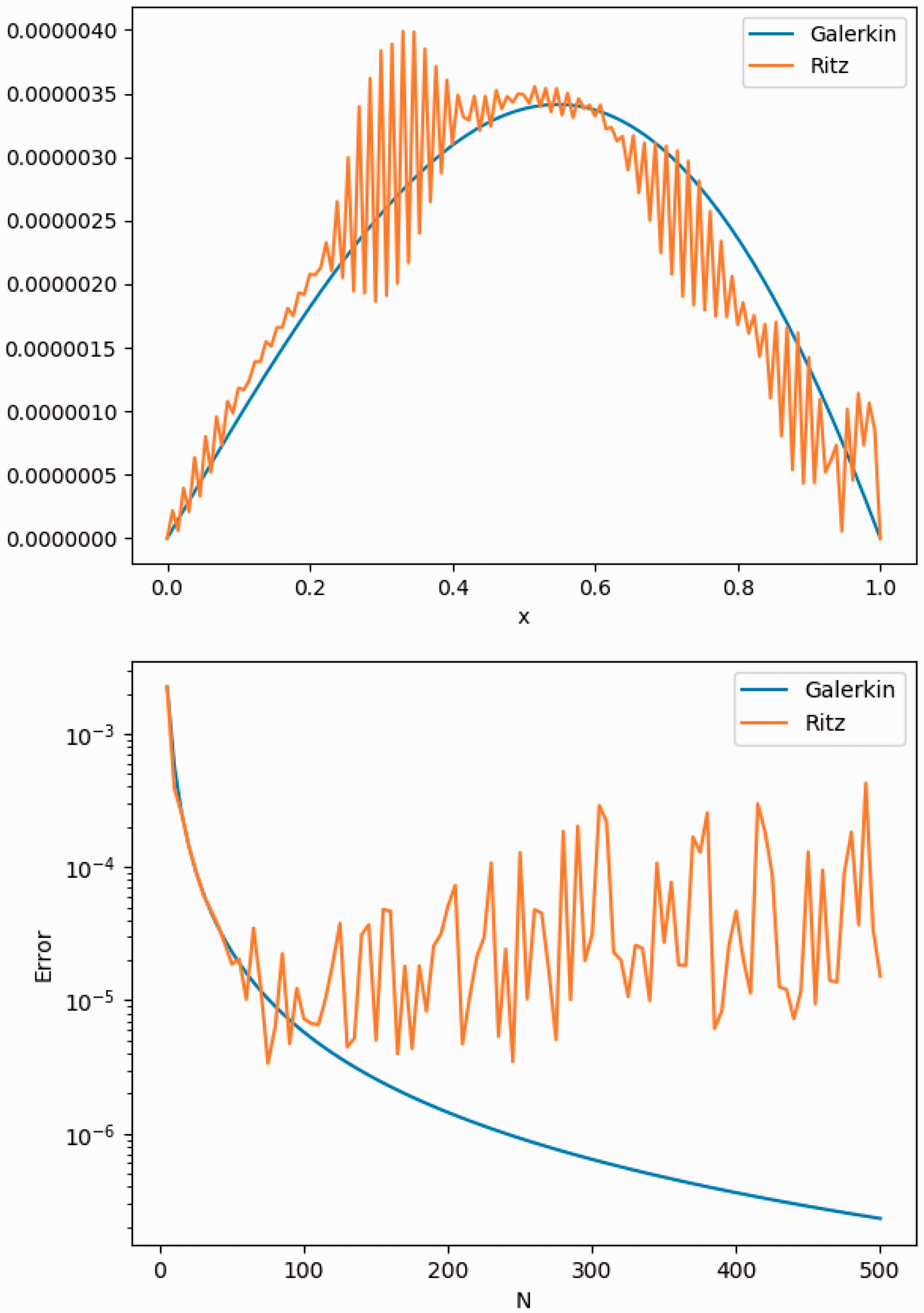It is found that the error decays as ${(1 / N)}^{2}$ for the conventional piecewise linear finite method, which is in a good agreement with a known theoretical estimate. However, the error stop decreasing with increasing N for the Ritz minimization method. This is probably due to the fact that the minimization algorithm fails to find the global minimizer. Instead, only local minimizers are found for large N. This is also one of main drawback of ANN method: increasing the dimension of the parameter space theoretically improves the best approximation, but not always improves the quality of the actual numerical solution because the best approximation is not always accessible by running the minimization algorithm.

Figure 1.

Upper: errors for the piecewise linear finite element method and Ritz minimization with 130 equidistance points. Lower: errors versus the grid number N.

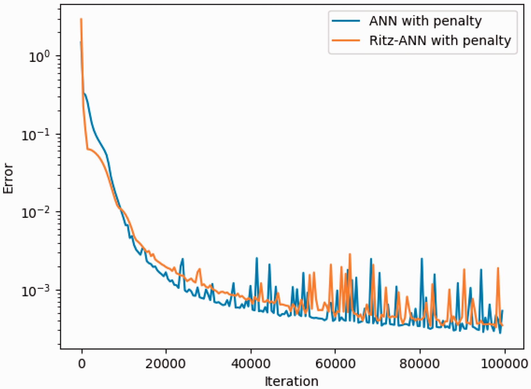
Next test concerns the performance of the ANN method, and the accuracy comparison among different loss functions. We will test the ANN method with the loss functions defined in (10), (11), (12), and (13). The error history versus the iteration number of the minimization algorithm is presented in Figure 2 for all four methods, i.e., ANN with exact BC (10), ANN with penalty (11), Ritz-ANN with exact BC (12), and Ritz-ANN with penalty (13). The calculation is performed with $N = 100, H = 16$ . In (11) we take β = 1, while in (13) we fix $β = 10^{3}$ . The ANN function used in (10) and (12) is constructed as

u_{p} (x) = x + x (x - 1) φ_{p} (x),

where

φ_{p} (x)

is given in (1).

Figure 2.

Error decay with respect to the iteration number for the loss functions (10), (11), (12), and (13).

From Figure 2 we can see that all four ANN methods generate numerical solutions with relatively high accuracy, which confirms the effectiveness of the ANN methods.

Also observed from this figure is that the error curves become flat or oscillating after about 20,000 iterations, which means that the minimization algorithm reaches the minimizer (probably local minimizer) at this iteration, and continuing running the algorithm does not improve the accuracy. The minimum errors captured during the iterations for different methods are listed in Table 1. As can be seen from this table, although the traditional Galerkin FEM has high accuracy dealing with this equation, some ANN methods, like (10) and (11), achieve higher accuracy with fewer parameters. It’s also obvious from this example that the accuracy of the natural ANN method is much higher than that of the Ritz ANN method. In the meanwhile, for the same type of the loss functions (natural or Ritz), a better accuracy is obtained if we enforce the numerical solution to exactly satisfy the boundary conditions. This experiment shows the superiority of enforcing the exact boundary conditions in the ANN function space compared to the penalty strategy. It is worth to point out that in the penalty formulations the choice of the penalty parameter β is an issue, and in some case, taking β = 1 in (13) for instance, the algorithm does not converge to the exact solution.

Table 1.

$L^{\infty}$ errors comparison among different methods.

Methods	Parameters	Errors
Galerkin-FEM	130	$3.41 \times 10^{- 6}$
Ritz-Functional	130	$3.98 \times 10^{- 6}$
ANN with exact BC	48	$1.18 \times 10^{- 6}$
ANN with penalty	48	$2.25 \times 10^{- 6}$
Ritz-ANN with exact BC	48	$1.92 \times 10^{- 3}$
Ritz-ANN with penalty	48	$8.59 \times 10^{- 3}$

Eaxmple 2 consider

{\begin{array}{l} - ε u ″ (x) + u' (x) = 0, x \in (0, 1), \\ u (0) = 0, u (1) = 1. \end{array}

The exact solution is $u (x) = \frac{e^{x / ε} - 1}{e^{1 / ε} - 1}$

Notice that the bilinear form associated to this example is no longer symmetric, so we can’t apply Ritz ANN methods in this situation. We will only compare the Galerkin method and the natural ANN method. First, we fix $ε = 0.1$ . The Galerkin FEM uses 100 grid points. In ANN we take $N = 100, H = 16$ . The penalty parameter β in (11) is fixed to 1. The errors of numerical solutions obtained by the Galerkin FEM (6), ANN with exact BC (10), and ANN with penalty (11) are plotted in Figure 3. We see that, as in Example 1, the accuracy of the numerical solution by the ANN method with even fewer parameters is better than the Galerkin FEM. It has been known that the Galerkin FEM with uniformly distributed grid points can’t well resolve the boundary layer of the solution, especially when ε is small. This demonstrates that the ANN has advantages over the conventional method for some difficult problems.

Figure 3.

Upper: pointwise errors for Galerkin method. Lower: $L^{\infty}$ errors versus the iteration number for the natural ANN methods when $ε = 0.1$ .

Then we test the accuracy for the same problem with a smaller ε, i.e., $ε = 0.05$ . In this situation, the exact solution exhibits a thinner boundary layer, which is harder to capture. The computed result is shown in Figure 4. It is observed from this figure that both methods produce lower accuracy, but the ANN method has more significant advantages over the conventional FEM.

Figure 4.

Upper: pointwise errors for Galerkin method. Lower: $L^{\infty}$ errors versus the iteration number for the natural ANN methods when $ε = 0.05$ .

In the following example, we will solve a two dimensional partial differential equation by the natural ANN and Ritz ANN methods, and compare their performance. Due to the difficulty of constructing exact boundary conditions for multiple dimensional problems or complex domains, we will only consider the loss functions (11) and (13). We take $N = 10^{2}$ uniformly distributed points in the domain as training points, and fix H = 16. The error behavior of the numerical solutions with respect to the iteration number is presented in Figure 5.

Figure 5.

Error evolution during the training process for Example 3.

Eaxmple 3 Consider:

{\begin{array}{l} - Δ u (x, y) = 0, (x, y) \in {(0, 1)}^{2}, \\ u (x, y) = x y, (x, y) \in \partial {(0, 1)}^{2} . \end{array}

The exact solution is $u (x, y) = x y$

It is readily seen from the presented numerical result that the minimization algorithm has almost same behavior for the two loss functions (11) and (13), and minimizing the two functions in the ANN function space gives almost same accuracy. This is in contrast with what we have observed in Example 1, where the result reported in Figure 1 showed that the accuracy of using (11) is better than that of (13). This seemingly contradictory result implies that the type of differential equations will affect the effectiveness of different ANN methods, and we would better not claim that one method is definitely better than others by only a few examples.

Parameter sensitivity investigation on single-layer network

In the previous section, we have shown by several examples that the ANN function has good approximation property, and minimizing suitable loss function (natural or Ritz type) in the ANN function space led to satisfying numerical solutions. We now turn to investigate how the ANN parameters have impact on the approximation property of the ANN function and on the convergence of the minimization algorithm. Before doing numerical experiments, a few things need to be stated in advance.

Firstly, we will use the examples tested in section ‘Comparative investigation among conventional, natural, and Ritz ANN methods’ for experiments. In each example, we fix the values of other parameters and only vary the parameter being tested. We will record the errors in $L^{\infty}$ norms through this process. Secondly, to be consistent with section ‘Comparative investigation among conventional, natural, and Ritz ANN methods’, we will always take 100² equidistant points in the domain as test points. Thirdly, in this section, the neural networks used are all single hidden layer with sigmoid activation functions.

For some differential equations whose operator $L$ and $B$ satisfy the Lipschitz condition, the error can be controlled by the value of loss function; see, e.g.,.²⁶ However in most cases, we don’t know how to predict the error of the numerical solution from the value of the loss function. Therefore, in the following numerical experiments, we are not concerned about the corresponding error when the loss function is at the minimum, but about the minimum error that can be achieved by adjusting the parameters during the training process.

Size of the training set

In this subsection, the network will be trained over a training set of equidistant points of increasing sizes. That is, we will increase the value of $N = 2^{k}, k = 2, 3, \dots, 10$ for Example 1 and 2, and $N = k^{2}, k = 5, 6, \dots, 15$ for Example 3. Then we observe how the errors in $L^{\infty}$ norms will react. Theoretically, the more training points, the smaller the error on the test points will be. Other parameters are fixed as follows: hidden layer nodes H = 16, activation function = Sigmoid, learning rate= $10^{- 3}$ , iteration = 100000. The errors as a function of the the number of training points are showed in Figure 6. We observe from this figure that for Examples 1 and 2, the error decreases with the number of training points at the beginning up to some value, but further increase of the training points does not allow to improve the accuracy. This observation suggests use of a moderate number of training points. It is notable that for Example 3, the number of training points seems have little impact on the error. In fact, highly accurate solutions have already been achieved by using a small number of training points. This is most likely due to the simple structure of the exact solution in this example.

Figure 6.

Errors of different methods versus the number of training points N. Upper: Example 1. Middle: Example 2 with $ε = 0.1$ . Lower: Example 3.

Number of nodes in hidden layer

In this subsection, the network will be trained over a fixed training set of equidistant points with increasing number of hidden layer nodes $H = 2^{k}, k = 2, 3, \dots, 8$ . The used parameters are: size of training set N = 100, activation function = Sigmoid, learning rate= $10^{- 3}$ , iteration = 100000. Figure 7 presents the error behavior versus the hidden layer nodes for different ANN methods.

Figure 7.

Errors versus the hidden layer nodes H for different methods. Upper: Example 1. Middle: Example 2 when $ε = 0.1$ . Lower: Example 3.

It is found that for Example 1, the maximum errors of the numerical solutions from all tested methods remain almost same when the hidden layer node H changes. This is probably due to the fact that the exact solution of Example 1, i.e., a trigonometric function, can be well approximated by only a few nodes. For Examples 2 and 3, the error decreases with increasing hidden layer node H at the beginning up to a value, then increases with increasing H. Notice that the solution space becomes larger as H increases, and theoretically more accurate solution should be found in a larger space. The numerical results given in Figure 7 seems to contradict with the theoretical prediction. To explain this contradiction, let’s emphasize that enlarging the solution space results in an increase of the local minimum, which makes the loss function easily fall into the local minimum. Furthermore, an excessively large solution space will cause overfitting, which will increase the error of the numerical solution at the test point.

Impact of the penalty parameter of loss function

This test concerns investigation of the impact of the penalty parameter used in loss function to deal with the boundary condition. As reported in section ‘Comparative investigation among conventional, natural, and Ritz ANN methods’, when we take β = 1 in (13), the numerical solutions lose accuracy dramatically in Example 1. When optimizing the loss function, the penalty parameter can be regarded as weights to the corresponding term, which plays a role to balance the satisfaction of the equation and boundary condition. Other parameters are fixed as in subsection ‘Number of nodes in hidden layer’. The errors respectively on the domain and the boundary versus the penalty parameter β are plotted in Figure 8. An interesting finding from this test is that increasing the penalty parameter results in damaging the accuracy of the natural ANN methods. This seems to indicate that for the natural ANN methods, we would better fix β to a smaller value to avoid possible lose of the accuracy. On the contrary, the Ritz ANN methods produce more accurate solution for relatively larger β, especially for Example 1. The accuracy of the Ritz ANN method is significantly improved as β gradually increases. However when the penalty parameter becomes extremely large, the same phenomenon as the natural ANN appears. This suggests use of a moderate penalty parameter, say $β = 10^{3}$ , in the Ritz ANN methods.

Figure 8.

Errors versus the penalty parameter β for different ANN methods. Upper: Example 1. Lower: Example 3.

Fitting a target function

In the previous section, we performed a series of sensitivity analyses on the parameters in the neural network algorithm for solving differential equations. As we have observed from the numerical experiments, different forms of loss function and the hyperparameters of ANN will affect the efficiency of the algorithm to find accurate numerical solutions. Theoretically, increasing the number of hyperparameters enlarges the ANN approximation space, and thus results in a better accuracy for the approximation to a given function. However we have seen that this did not equally lead to a better accuracy of the numerical solution as expected in some of the numerical examples. This is one of our key observations from the previous numerical tests, which we want to further understand here. Apparently the efficiency of the ANN methods is related not only to the form of the loss function, but also to the feature of the exact solution. Therefore, in this section we aim at studying the approximation behavior of the ANN methods to target functions using different activation functions, and characterizing the training process in approximating specific functions.

Given a function f, an ANN approximation consists in finding suitable parameters p that minimizes the loss function:

J (p) = \frac{1}{N} \sum_{i = 1}^{N} {(φ_{p} (x_{i}) - f (x_{i}))}^{2},

(14)

where

{x_{i}}

is a set of the training points.

For fitting functions with neural networks, Barron¹⁸ proved that the mean integrated squared error between the output of the network and the target function is bounded by $O (\frac{c}{H}) + O (\frac{H d}{N} \log N)$ , where H is the number of hidden layer nodes, d is the dimension of the input data for the function, N is the number of training points and c is a constant which depends on the target function. The two terms correspond respectively to the approximation error and the estimation error.

Choice of activation function

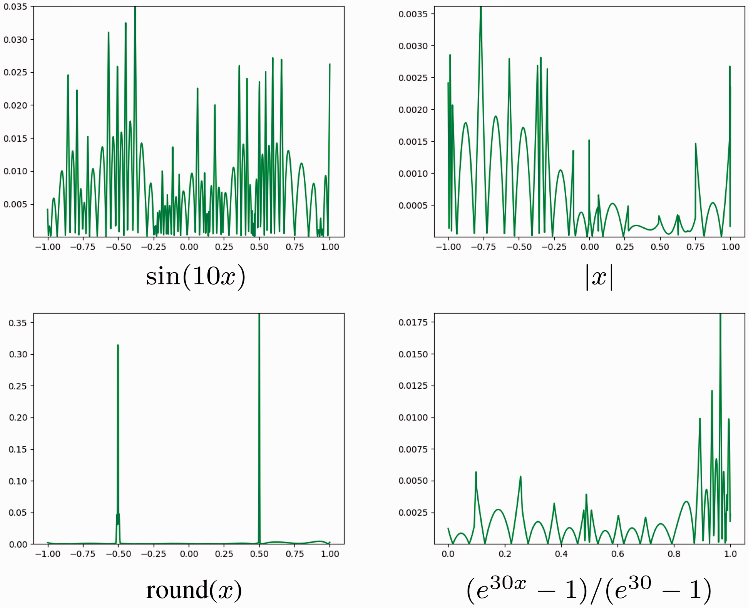
In this subsection, we want to figure out whether an activation is suitable to approximate the target function and how shall we choose the activation function according to the target function. We will use the following functions as examples to test the effect of ANN in fitting functions.

\begin{array}{l} f_{1} (x) = \sin (10 x), x \in [- 1, 1], \\ f_{2} (x) = | x |, x \in [- 1, 1], \\ f_{3} (x) = round (x), x \in [- 1, 1], \\ f_{4} (x) = \frac{e^{30 x} - 1}{e^{30} - 1}, x \in [0, 1] . \end{array}

The above target functions have their own characteristics respectively. Among them, $f_{1} (x)$ is smooth in the domain; $f_{2} (x)$ does not exist derivative at zero, but is differentiable in the rest of the domain; $f_{3} (x)$ has discontinuities in the domain; $f_{4} (x)$ is smooth in the domain, but value increases sharply at the right end of the interval. The hyperparameters are fixed as follows: N = 64 for $f_{1}, f_{2}, f_{4}$ and N = 1000 for f₃, H = 16, iteration = 50,000 learning rate= $10^{- 3}$ , and 1000 test points uniformly selected from the interval.

We first test for a sigmoidal function, and the result is presented in Figure 9. We can observe from this figure that when the target function is smooth, the accuracy is quite satisfying. When there exists a discontinuous point or a non-differentiable point, the ANN method results in a less precise approximation. Nevertheless, it is notable that the effect of the discontinuity on the precision seems to be local. That is, the precision remains satisfying outside a small region surrounding the discontinuities or large gradient. This is one of the superiorities of ANN methods compared to conventional approximations in which the effect of the discontinuity is often global.

Figure 9.

Fitting errors of ANN methods for four functions with a sigmoidal activation function.

We then test for the Relu function, i.e., $σ (x) = \max {0, x}$ , in the ANN fitting method. The computed result is given in Figure 10. The error curves in the figure show that the approximation accuracy is lower as compared to the sigmoidal basis function for smooth functions. On the contrary, the Relu basis function performs better than the sigmoidal basis function for the target functions non-derivable or having discontinuous. This phenomena can be clearly explained by the fact that the Relu basis function itself is less smoother than the sigmoidal basis function.

Figure 10.

Fitting errors of ANN methods for four functions with the Relu activation function.

These observations motivate us to consider a compromise: constructing a mixed ANN approximation using both Relu and sigmoidal basis functions. It is expected that such a mixed ANN may take the advantages from both activation functions. To this end, we divide the hidden layer into two parts, and use the sigmoidal basis function in one part and the Relu basis function in another. More precisely, we construct the mixed ANN as follows:

φ_{p} (x) = \sum_{i = 1}^{\frac{H}{2}} \frac{a_{i}}{1 + e^{- (w_{i} x + b_{i})}} + \sum_{i = \frac{H}{2} + 1}^{H} a_{i} \max {0, w_{i} x + b_{i}}

where

w_{i} \in R^{n}, a_{i}, b_{i} \in R

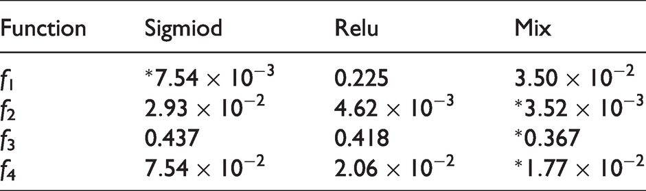
Figure 11 shows the fitting result by using the mixed ANN. It is clearly seen that, except of the first target function for which the sigmoidal basis function produces a little lit better accuracy, the mixed network improves the accuracy for all other three target functions, especially for the second.

Figure 11.

Fitting errors of ANN method with the mixed activation function.

We present some more details of the above experiments in Table 2, from which it becomes clear that the mixed ANN is most accurate for almost all tested target functions.

Table 2.

$L^{\infty}$ errors: accuracy comparison for different activation functions.” *” marks the best accuracy.

Function	Sigmiod	Relu	Mix
f ₁	$^{*} 7.54 \times 10^{- 3}$	0.225	$3.50 \times 10^{- 2}$
f ₂	$2.93 \times 10^{- 2}$	$4.62 \times 10^{- 3}$	$^{*} 3.52 \times 10^{- 3}$
f ₃	0.437	0.418	$^{*} 0.367$
f ₄	$7.54 \times 10^{- 2}$	$2.06 \times 10^{- 2}$	$^{*} 1.77 \times 10^{- 2}$

Fitting Müntz polynomials

Müntz polynomials show unique advantages in many situations, whose application covers a large number of problems. In particular, it has been found²⁷ that the Müntz polynomials can more accurately approximate the solution of some equations, such as integro-differential equations, fractional differential equations, and so on, than the traditional polynomials. In this subsection we aim at investigating the capability of ANN methods to approximate Müntz polynomials. This can be regarded as the first step toward constructing efficient ANN methods to solve integro-fractional differential equations.

A n terms Müntz polynomial can be written as $\sum_{i = 1}^{n} α_{i} x^{λ_{i}}, x \in (0, \infty)$ , where $α_{i} \in R$ is the coefficients, and $λ_{i} \in R^{+}$ is the powers. The idea is to propose an ANN based on Müntz polynomials to approximate a given Müntz polynomial, and it is interesting to see if such an ANN is capable of correctly capturing the coefficients and the powers. Precisely, the proposed ANN method consists in seeking the parameter $p : = {w_{i}, a_{i}}$ , which minimizes the loss function:

J (p) = \frac{1}{N} \sum_{i = 1}^{N} {(\sum_{j = 1}^{n} a_{j} x_{i}^{w_{j}} - \sum_{j = 1}^{n} α_{j} x_{i}^{λ_{j}})}^{2},

where N represents the number of training points. For a Müntz polynomial with n terms, if we use a neural network with n hidden layer nodes, in principle we can get the exact target function. The numerical experiment carried out in this subsection has the purpose of testing the capability of ANN methods of this structure. We still use the AdamOptimizer to optimize the loss function. In what follows we fix N to 20, learning rate to

10^{- 3}

, iteration number to 100000.

Eaxmple 4

f (x) = (\sqrt{3} + 1) x^{- 2} - 0.8 x^{\sqrt{2}}, x \in [1, 2]

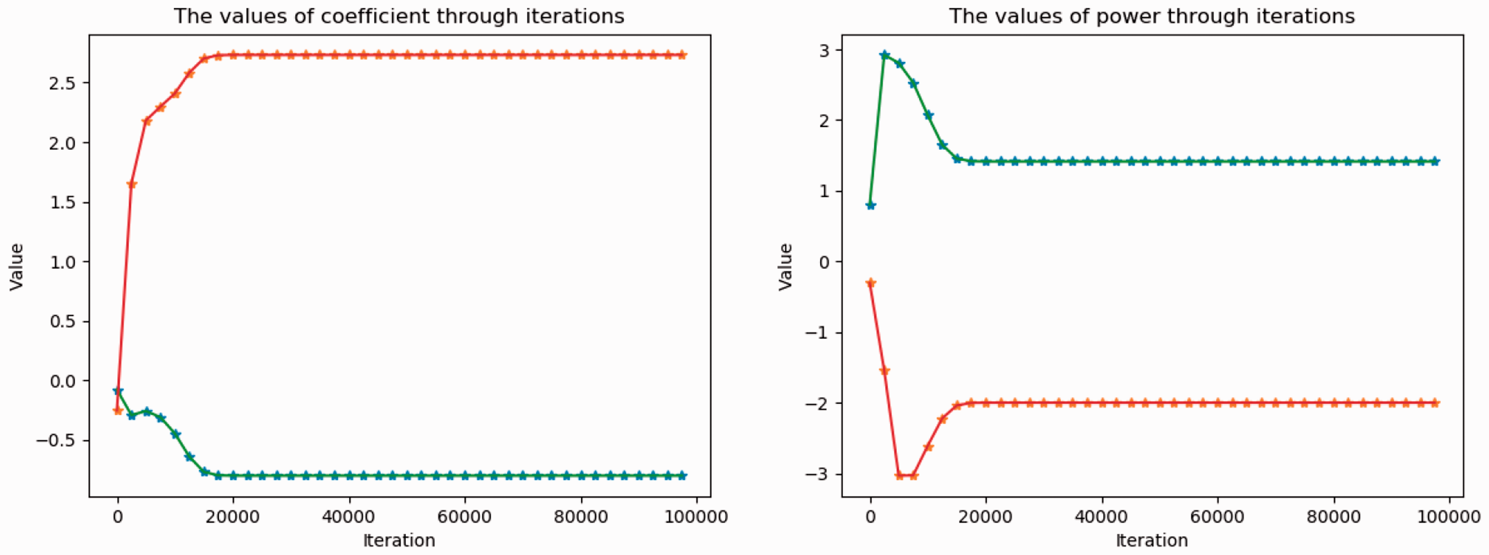
There are only two terms in this Müntz polynomial, therefore there are two coefficients and two power values to be optimized in the neural network. Figure 12 shows parameter fitting during the training process. We can readily see that after 20,000 iterations, both the power w_j and the coefficient parameter a_j in the neural network gradually stabilizes at their exact values, i.e., –2 and $\sqrt{2}$ for w_j and $\sqrt{3} + 1$ and −0.8 for a_j, respectively.

Figure 12.

Parameter fitting during the training process for Example 4.

Figure 13.

Errors of the convergent solution for Example 4 and Example 5.

Example 4 showed how the neural network learns each parameter step by step, and precisely find the parameters of the target function. Now we consider a three-term Müntz polynomial in Example 5. The corresponding result is presented in Figures 13 and 14. Surprisingly, although the approximation error remains good enough, the networks fails to find the exact parameters of the target function, neither the coefficients nor the powers. A reasonable explanation for this failure is that increasing the number of terms, which means increasing the parameter space, makes the number of local or global minimum larger. 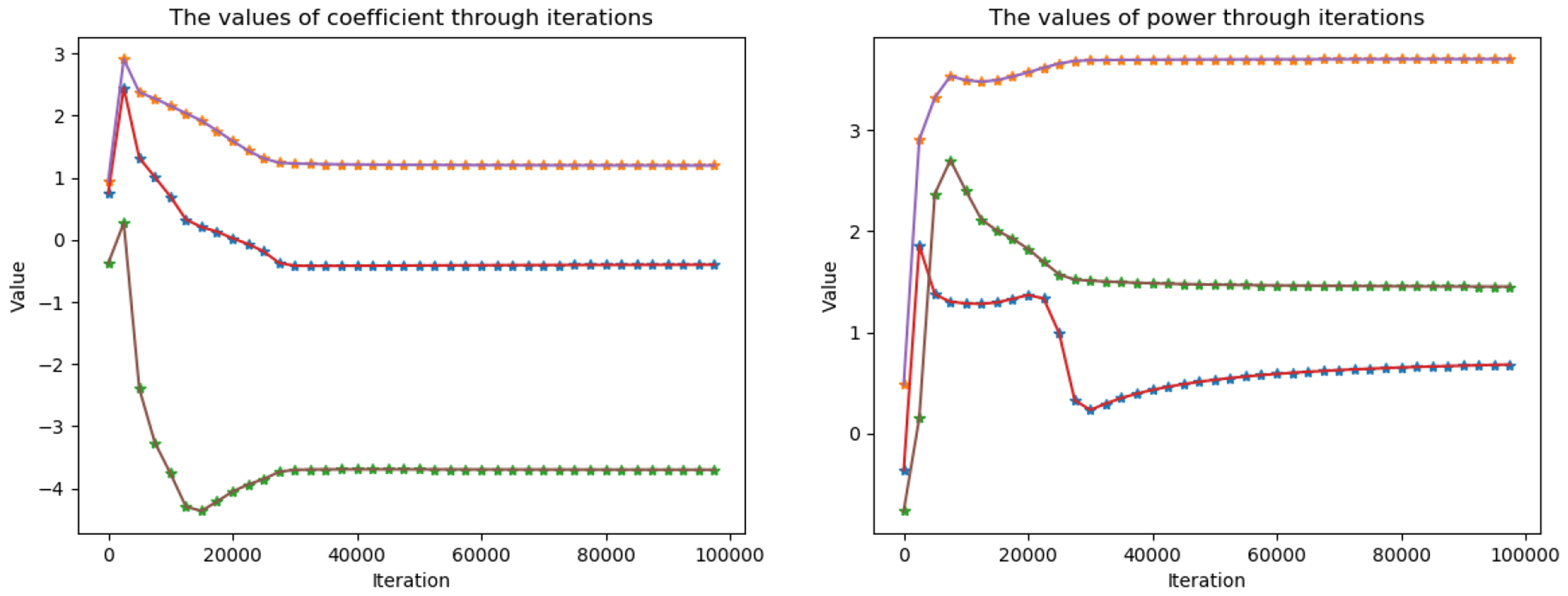In fact, it can be directly checked that for a Müntz polynomial with n terms, there are $n!$ global minimums in the solution space. The current minimization algorithm in use has no guarantee of finding a global minimizer among multi-minimizers (local or global).

Figure 14.

Parameter fitting during the training process for Example 5.

Eaxmple 5

f (x) = 1.2 x^{3.7} - 3.1 x^{1.5} - x, x \in [0.5, 5]

Conclusion and discussion

In this paper, we have discussed possible forms of loss functions in an ANN method for solving differential equations, and investigated their efficiency through a number of numerical examples. In particular, a comparative investigation was carried out between the natural ANN and Ritz ANN methods, and between the penalty strategy and imposing the exact boundary condition in the ANN function space. The sensitivity on the accuracy of the ANN methods with respect to the size of training set, the number of nodes in hidden layer, as well as the penalty parameter was also studied. Finally, in order to better understand the training behavior of the proposed neural networks, we have selected several types of functions, and studied their approximation properties by the ANN methods.

Although no decisive conclusion was reached regarding the choices of loss functions or activation functions, some interesting points can be drawn from our numerical study:

– in most of our tests, the natural ANN has demonstrated its superiority compared to the Ritz ANN;

– an ANN with exact boundary conditions is more accurate than an ANN with penalty;

– smooth activation function is preferable over nonsmooth activation function in approximating smooth functions. On the contrary, it is better to use nonsmooth activation function such as Relu in approximating nonsmooth functions. Generally, mixed use of smooth and nonsmooth activation function is recommended.

– the proposed Müntz ANN is only capable of finding few-term Müntz polynomials, more investigation is needed to see how an ANN can be trained to find a general Müntz polynomials.

The numerical experiments carried out in the current paper did not give a solid mathematical foundation to ANN for solving differential equations, but might provide guidance for subsequent theoretical analysis. As part of the future work, we will try to study the convexity of different forms of loss functions under specific examples. Another interesting direction that is worth exploring is to establish the relationship between loss function and errors.

Footnotes

Declaration of Conflicting Interests

The author(s) declared no potential conflicts of interest with respect to the research, authorship, and/or publication of this article.

Funding

The author(s) disclosed receipt of the following financial support for the research, authorship, and/or publication of this article: The research of the authors is partially supported by NSFC grant 11971408, NNW2018-ZT4A06 project, and NSFC/ANR joint program 51661135011/ANR-16-CE40-0026–01.

ORCID iD

Chuanju Xu

References

Evans

LC.

Partial differential equations. 2nd ed. Providence: American Mathematical Society, 2010.

Alfio

Alberto

Numerical approximation of partial differential equations. In Springer series in computational mathematics, 2008, Vol.23. Springer Science & Business Media.

Dret

Lucquin

Partial differential equations – modeling, analysis and numerical approximation. Basel, Switzerland: Birkhauser, 2016.

Bartels

Numerical approximation of partial differential equations. Berlin: Springer, 2016.

Lee

Kang

IS.

Neural algorithm for solving differential equations. J Comput Phys 1990; 91: 110–131.

Meade

Jr and Fernandez

AA.

The numerical solution of linear ordinary differential equations by feed forward neural networks. Math Comput Modell 1994; 19: 1–25.

Meade

Jr and Fernandez

AA.

Solution of nonlinear ordinary differential equations by feedforward neural networks. Math Comput Modell 1994; 20: 19–44.

Chiaramonte

Kiener

Solving differential equations using neural networks, Project document, 2013.

Lagaris

Likas

Fotiadis

DI.

Artificial neural networks for solving ordinary and partial differential equations. IEEE Trans Neural Netw 1998; 9: 987–1000.

10.

Lagaris

Likas

Papageorgiou

DG.

Neural network methods for boundary value problems with irregular boundaries. IEEE Trans Neural Netw 2000; 11: 1041–1049.

11.

Mall

Chakraverty

Application of Legendre neural network for solving ordinary differential equations. Appl Soft Comput 2016; 43: 347–356.

12.

McCaffray

Gallant

AR.

Convergence rates for single hidden layer feedforward networks. Neural Netw 1994; 7: 147–158.

13.

Justin

Konstantinos

DGM: a deep learning algorithm for solving partial differential equations. J. Comput. Phys, 2018; 375: 1339–1364.

14.

Weinan

The deep Ritz method: a deep learning-based numerical algorithm for solving variational problems. Commun Math Stat 2018; 6: 1–12.

15.

Michoski

Milosavljevic

Oliver

, et al. Solving differential equations using deep neural networks. Neurocomputing 2020; 399: 193–212.

16.

Glorot X and Bengio Y. Understanding the difficulty of training deep feedforward neural networks. In: Proceedings of the 13th international conference on artificial intelligence and statistics (AISTATS), Vol.9, Chia Laguna Resort, Sardinia, Italy, 13-15 May,2010, pp. 249–256.

17.

Cybenko

GV.

Approximation by superpositions of a sigmoidal function. In: van Schuppen JH (ed) Mathematics of control, signals, and systems. Berlin: Springer International, 1989, pp.303–314.

18.

Barron

AR.

Approximation and estimation bounds for artificial neural networks. Mach Learn 1994; 14: 115–133.

19.

Barron

AR.

Universal approximation bounds for superpositions of a sigmoidal function. IEEE Trans Inform Theory 1993; 39: 930–945.

20.

Lewicki

Marino

Approximation by superpositions of a sigmoidal function. J Anal Appl 2003; 22: 463–470.

21.

Pakdaman

Ahmadian

Effati

, et al. Solving differential equations of fractional order using an optimization technique based on training artificial neural network. Appl Math Comput 2017; 293: 81–95.

22.

Piscopo

Spannowsky

Waite

Solving differential equations with neural networks: applications to the calculation of cosmological phase transitions. Phys Rev D 2019; 100: 016002.

23.

Shen

Yang

Zhang

Deep network approximation charactized by number of neurons. Commun Compu Phys 2020; 28:1768–1811.

24.

ZQJ

Zhang

Xiao

Training behavior of deep neural network in frequency domain. International Conference On Neural Information Processing (ICONIP) 2019; 11953: 264–274.

25.

Shen

Tang

Wang

LL.

Spectral methods: algorithms, analysis and applications. Berlin: Springer, 2011.

26.

Remco van der Meer

Oosterlee

Borovykh

Optimally weighted loss functions for solving PDEs with neural networks. arXiv e-print, arXiv: 2002.06269v3, 2020.

27.

Hou D, Lin Y, Azaiez M, et al. A Müntz-collocation spectral method for weakly singular volterra integral equations. J Sci Comput 2019; 81: 2162–2187.

A comparative investigation of neural networks in solving differential equations

Abstract

Keywords

Introduction

Artificial neural networks and choices of loss function

Conventional numerical methods

Natural ANN method

Ritz ANN method

Comparative investigation among conventional, natural, and Ritz ANN methods

Parameter sensitivity investigation on single-layer network

Size of the training set

Number of nodes in hidden layer

Impact of the penalty parameter of loss function

Fitting a target function

Choice of activation function

Fitting Müntz polynomials

Conclusion and discussion

Footnotes

Declaration of Conflicting Interests

Funding

ORCID iD

References