Keeping it together: A phase-field version of path-connectedness and its implementation

Abstract

We describe the implementation of a topological constraint in finite-element simulations of phase-field models, which ensures path-connectedness of preimages of intervals in the phase-field variable. The constraint takes the form of an energetic penalty for a suitable geodesic distance between all pairs of points in the domain. The main application of our method presented here is a discrete steepest descent of a phase-field version of a bending energy with spontaneous curvature and additional surface area penalty. This leads to disconnected surfaces without our topological constraint but connected surfaces with the constraint. Numerically, our constraint is treated by first transforming the double integral over all pairs of points in the domain to a weighted graph structure and then using Dijkstra’s algorithm to calculate the distance between discrete connected components.

Introduction

In this article, we describe how to incorporate a topological constraint into a phase-field simulation for certain geometric functionals. In three dimensions (3D), the prototypical example of such an energy is Willmore’s energy, that is, the integral of mean curvature squared, restricted to the class of $C^2$ -manifolds embedded into a bounded domain $\mathrm{\Omega }\subset {\mathbb{R}}^3$ such that the embedding has surface area $S>0$ and is connected. A number of more general functionals are also admissible – the precise theoretical setting for our methods is presented in section ‘Geometric energies’. It is also possible to use our algorithm in the case of functionals controlling only the perimeter of sets contained in a bounded domain $\mathrm{\Omega }\subset {\mathbb{R}}^2$ .^1,2 To simplify the presentation, we focus here on the 3D case with a control of Willmore’s energy.

Our method to enforce this connectedness constraint for diffuse interfaces is based on a functional ${\mathcal{C}}_{\epsilon }$ introduced in Dondl et al. ³ and given by

$${\mathcal{C}}_{\epsilon }(u)={\int }_{\mathrm{\Omega }\times \mathrm{\Omega }}\frac{1}{\epsilon }\tilde{W}(u(x))\frac{1}{\epsilon }\tilde{W}(u(y))d^{F(u)}(x,y)\mathrm{d}x\mathrm{d}y$$

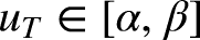
where $\tilde{W},F$ are continuous functions such that

$$\tilde{W},F\ge 0,F(z)=0\iff z\in [\alpha ,\beta ],\tilde{W}(z)>0\iff z\in (\alpha ,\beta )$$

for some $-1<\alpha <\beta <1$ and

$$d^{F(u)}(x,y)=inf\left\{{\int }_{\gamma }F(u)\mathrm{d}{\mathcal{H}}^1|\gamma \mathrm{curve}\mathrm{from}x\mathrm{to}y\right\}$$

is a geodesic distance function. For a heuristic interpretation of the functional, see section ‘The topological term’ and Figure 1.

Figure 1.

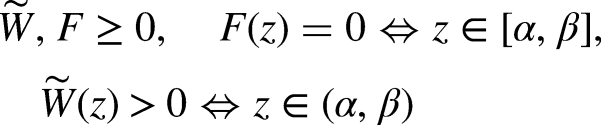
The transition profile $\varphi$ (green) of a phase field $u$ viewed orthogonal to the level sets and typical weight functions $\tilde{W}(\varphi )$ for the integral (red) and $F(\varphi )$ for the geodesic distance (blue). If the pre-image $u^{-1}(\alpha ,\beta )$ is connected, then every two points in the pre-image can be connected by a curve of weighted length zero.

Despite the intimidating appearance of the functional ${\mathcal{C}}_{\epsilon }$ as a double integral coupled to a geodesic distance, an efficient algorithm to treat this term can be implemented. We rely on a decomposition into connected components and a Dijkstra or fast marching-type method to approximate the geodesic distance as well as its variation. An important change compared to previous work(e.g. Bonnivard et al. ⁴ ) is a decomposition due to the fact that the distance function in the discrete setting introduced in section ‘Discretizing the geodesic distance’ is exactly zero among all points in one component. This allows us to transform the double integral into a sum of (usually) only a few terms, which enables us to treat the topology in phase-field problems efficiently, even in 3D and in a setting where not only connectedness between a finite set of fixed points is enforced.

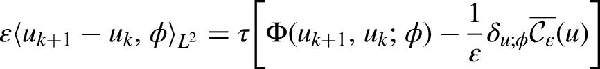
In our simulations, we compute a discrete-time gradient flow (approximately) solving in each time step the minimization problem

$$u_{n+1}\in \mathrm{argmin}(u\mapsto \frac{\epsilon }{2\tau }\Vert u-u_n{\Vert }_{L^2(\mathrm{\Omega })}^2+{\mathcal{F}}_{\epsilon }(u)+\frac{a}{\epsilon }{\mathcal{C}}_{\epsilon }(u))$$

(1)

where ${\mathcal{F}}_{\epsilon }$ is an admissible phase-field approximation of a geometric functional $\mathcal{F}$ and $a\ge 0$ is a constant. Note that the case $a=0$ of course provides no penalty for disconnectedness. The parameter $\tau >0$ is the size of a discrete time step in this minimizing movements scheme.

To the best of our knowledge, this is the first practical method that can incorporate a connectedness constraint for evolving surfaces in 3D into phase-field simulations. This compares to previous work, for example, in Bonnivard et al. ⁴ and Chambolle et al., ⁵ where Steiner-tree-type problems (i.e. keeping connected a fixed set of points) in two space dimensions were addressed using phase fields.

The article is structured as follows. In section ‘Geometric energies’, we recall precise statements regarding the sharp interface limit of functionals of the form ${\mathcal{F}}_{\epsilon }+\frac{1}{\epsilon }{\mathcal{C}}_{\epsilon }$ , where ${\mathcal{F}}_{\epsilon }$ is a term controlling a diffuse version of Willmore’s energy as well as the perimeter.^6,7 In the following parts of section ‘Preliminaries’, we give a heuristic explanation of our topological functional and briefly review the background material on the distance function on graphs which will be required below. In section ‘The algorithm’, we describe an implementation of the connectedness constraint. In section ‘Numerical results’, we present simulations with and without the topological constraint.

Preliminaries

Geometric energies

Our main numerical example in this article is the treatment of the functional

$$\begin{array}{rl}{\mathcal{F}}_{\epsilon }(u)& ={\mathcal{W}}_{\epsilon }(u)+\lambda S_{\epsilon }(u)\\ & =\frac{1}{c_0\epsilon }{\int }_{\mathrm{\Omega }}{(-\epsilon \mathrm{\Delta }u-\frac{1}{\epsilon }{W}^{\prime }(u)-H_0\sqrt{2W(u)})}^2\mathrm{d}x\\ & +\lambda \frac{1}{c_0}{\int }_{\mathrm{\Omega }}\frac{\epsilon }{2}|\mathrm{\nabla }u{|}^2+\frac{1}{\epsilon }W(u)\mathrm{d}x\end{array}$$

(2)

with $\lambda >0$ and $H_0\in \mathbb{R}$ in three ambient space dimensions. For $c_0={\int }_{-1}^1\sqrt{2W(s)}\mathrm{d}s$ and $W(u)=\frac{1}{4}(u^2-1{)}^2$ , this functional approximates the sum of curvature energy and surface area

$$\mathcal{F}(\mathrm{\Sigma })={\int }_{\mathrm{\Sigma }}|H-H_0{|}^2\mathrm{d}A+\lambda {\int }_{\mathrm{\Sigma }}1\mathrm{d}A$$

(3)

if $\mathrm{\Sigma }$ is a $C^2$ surface in $\mathrm{\Omega }$ with mean curvature $H$ and area element $\mathrm{d}A$ . If $H_0=0$ , this can be made rigorous in the sense of $\mathrm{\Gamma }$ convergence, while the situation is more complicated for $H_0\ne 0$ . We refer the reader to Röger and Schätzle, ⁷ Dondl et al. ³ and Bellettini and Mugnai ⁶ for a more detailed account of the convergence results. The curvature energy in (3) has been proposed as a model for the bending of thin membranes.^8,9 In such a phase-field computation, the zero level set $\{u=0\}$ is usually interpreted as an approximation for the surface $\mathrm{\Sigma }$ .

The simplified geometric model does not control other physical aspects of the membranes. In applications concerning mitochondrial membranes, the surface $\mathrm{\Sigma }$ is typically connected and the boundary of a connected subset of $\mathrm{\Omega }$ . The phase-field model naturally incorporates the aspect that $\mathrm{\Sigma }$ should be a boundary, and boundary conditions for $u$ can be used to ensure that $\mathrm{\Sigma }$ touches $\mathrm{\partial }\mathrm{\Omega }$ only tangentially. In this article, we describe how to furthermore incorporate the connectedness constraint in computational methods for purely geometric models. Note however that we retain the flexibility of phase-field models for other topological transitions (changes of genus).

The topological term

Functions for which ${\mathcal{F}}_{\epsilon }$ is finite are continuous in dimensions $n=2,3$ due to Sobolev embeddings, so the following notions are well-defined. While, usually, the interface is approximated by the zero level set $\{u=0\}$ , it is equivalent to approximate it by the pre-image of any interval $(\alpha ,\beta )⋐(-1,1)$ , for a precise statement see Dondl and Wojtowytsch ¹⁰ Theorem 2.20. Thus it is possible to introduce a quantitative notion of path-connectedness of the interface $I:=u{}^{-1}(\alpha ,\beta )$ at two points $x,y\in I$ through a geodesic distance function

$$d^{F(u)}(x,y)=inf\left\{{\int }_{\gamma }F(u)\mathrm{d}{\mathcal{H}}^1|\gamma \mathrm{curve}\mathrm{from}x\mathrm{to}y\right\}$$

with a weight $F(u)$ satisfying

$$F\in C^1(\mathbb{R}),F\equiv 0\mathrm{on}[\alpha ,\beta ],F>0\mathrm{outside}[\alpha ,\beta ]$$

In particular, if $I$ is (path-)connected, then $d^{F(u)}(x,y)=0$ for all $x,y\in I$ . If, however, there are multiple connected components of $I$ with a positive spatial separation, then any curve $\gamma$ should have a uniformly positive length between $x$ and $y$ if the two points are in different connected components. We now measure the total disconnectedness of $I$ by a double integral of the quantitative path-disconnectedness of $I$ at $x$ and $y$ over the entire interface with respect to both $x$ and $y$

$${\mathcal{C}}_{\epsilon }(u)={\int }_{\mathrm{\Omega }\times \mathrm{\Omega }}\frac{1}{\epsilon }\tilde{W}(u(x))\frac{1}{\epsilon }\tilde{W}(u(y))d^{F(u)}(x,y)\mathrm{d}x\mathrm{d}y$$

where $\tilde{W}$ is a bump function

$$\tilde{W}\in C^1(\mathbb{R}),\tilde{W}>0\mathrm{on}(\alpha ,\beta ),\tilde{W}\equiv 0\mathrm{outside}(\alpha ,\beta ).$$

The dependence of ${\mathcal{C}}_{\epsilon }$ on the choices of $F$ and $\tilde{W}$ , and therefore on $\alpha$ and $\beta$ , should be kept in mind, but for notational convenience, we will not make it explicit in the remainder of this article. Along the usual optimal profile recovery sequence for a connected, smooth, embedded manifold, ${\mathcal{C}}_{\epsilon }$ vanishes identically. The bound on ${\mathcal{W}}_{\epsilon }+S_{\epsilon }$ enforces a strong mode of convergence for $u_{\epsilon }$ to $\pm 1$ away from $\mathrm{spt}\mu$ , which suffices for ${\mathcal{C}}_{\epsilon }$ to detect a disconnected interface in the sense that $lim inf{\mathcal{C}}_{\epsilon }(u_{\epsilon })>0$ if $\mu$ has more than one connected component, see Dondl et al. ³ and Dondl and Wojtowytsch. ¹⁰ The normalization factor $\frac{1}{\epsilon }$ is used since an interface has a width proportional to $\epsilon$ .

We note that the topological penalty term ${\mathcal{C}}_{\epsilon }$ vanishes when approximating $C^2$ surfaces for small $\epsilon >0$ . It therefore does not change the behaviour of ${\mathcal{F}}_{\epsilon }$ in the situations that we are interested in.

Remark 1

The double-well potential $\tilde{W}$ depends on $W$ only in the sense that $\mathrm{supp}(\tilde{W})$ must lie strictly between the wells of $W$ , and furthermore that multiple topological functionals ${\mathcal{C}}_{\epsilon }^{+},{\mathcal{C}}_{\epsilon }^{-}$ can be used to keep level sets $u^{-1}({\alpha }^{+},{\beta }^{+})$ and $u^{-1}({\alpha }^{-},{\beta }^{-})$ connected for different ${\alpha }^{+}<{\beta }^{+}$ and ${\alpha }^{-}<{\beta }^{-}$ , for example a level set close to $+1$ and another one close to $-1$ . This will be useful for the numerical implementation later.

Discretizing the geodesic distance

Let $\mathrm{\Gamma }$ be a finite connected (undirected) graph with vertices $v$ and edges $e$ that are assigned weights $w_e\ge 0$ . The distance of two vertices $v,v^{\prime }$ is defined by the length of the shortest path in the graph connecting $v$ and $v^{\prime }$ where the length of an edge $e$ is measured by the weight $w_e$ , that is

$$\begin{array}{rl}& d(v,v^{\mathrm{\prime }})\\ & =inf\left\{\sum _{i=1}^n{w}_{e_i}|v=v_0,v^{\mathrm{\prime }}=v_n,v_{i-1},v_i\in e_i,n\in \mathbb{N}\right\}.\end{array}$$

In our finite-element setting, we consider a sequence of quasi-uniform triangulations (or tetrahedralizations in 3D) ${\mathcal{T}}_h$ of our domain $\mathrm{\Omega }$ with a spatial grid scale $h$ for $h\to 0$ . We furthermore assume that $u$ is a given continuous function on $\mathrm{\Omega }$ . Let now ${\mathrm{\Gamma }}_h(u)$ be the dual graph associated with a tesselation ${\mathcal{T}}_h$ , that is, a vertex $v$ of ${\mathrm{\Gamma }}_h(u)$ corresponds bijectively to a triangle or tet (i.e. tetrahedron) $T=T_v\in {\mathcal{T}}_h$ and that if $T_1\in {\mathcal{T}}_h$ shares an edge (or a face in 3D) with $T_2\in {\mathcal{T}}_h$ , then the corresponding vertices in ${\mathrm{\Gamma }}_h(u)$ are connected by an edge. To such an edge $e=e(T_1,T_2)$ , we associate the weight $w_e(u_{T_1},u_{T_2})=[F(u_{T_1})+F(u_{T_2})]/2\cdot [\mathrm{diam}(T_1)+\mathrm{diam}(T_2)]/2$ , where $u_T=\frac{1}{|T|}{\int }_{T}u\mathrm{d}x=:-{\int }_{T}u\mathrm{d}x$ . This gives rise to a discrete distance $d^{{\mathrm{\Gamma }}_h(u)}$ depending on a phase-field function $u$ . We denote by $d^{{\mathrm{\Gamma }}_h(u)}(T,T^{\prime })$ the distance between individual tets/triangles and by ${\mathrm{dist}}^{{\mathrm{\Gamma }}_h(u)}(C,C^{\prime })=inf\{d^{{\mathrm{\Gamma }}_h(u)}(T,T^{\prime })\mathrm{for}T\in C,T^{\prime }\in C^{\prime }\}$ the distance between sets.

The tesselations may force a minimal path to zig-zag to connect two points, so the distance on the graph may not approximate the distance function

$$d^{F(u)}(x,y)=inf\left\{{\int }_{\gamma }F(u)\mathrm{d}{\mathcal{H}}^1|\gamma \mathrm{curve}\mathrm{from}x\mathrm{to}y\right\},$$

as $h\to 0$ , but, due to the non-degeneracy assumptions on the tesselation and the $W^{2,2}$ -bound on $u$ , we note that the discrete distance $d^{{\mathrm{\Gamma }}_h(u)}$ is equivalent to $d^{F(u)}$ in an almost bi-Lipschitz sense uniformly in $h$ , that is

$$c{d}^{{\mathrm{\Gamma }}_h(u)}(T,T^{\prime })-\overline{c}h\le d^{F(u)}(x,x^{\prime })\le C{d}^{{\mathrm{\Gamma }}_h(u)}(T,T^{\prime })+\overline{C}h$$

for all $x,x^{\prime }\in \mathrm{\Omega }$ and $T,T^{\prime }\in {\mathcal{T}}_h$ such that $x\in T,x^{\prime }\in T^{\prime }$ with suitable constants $c,\overline{c},C,\overline{C}$ . This can be seen as follows: If $x,x^{\prime }$ lie in the same tet, then their distance is at most $\overline{C}h$ , and the estimate holds trivially. If $x,x^{\prime }$ lie at the boundary of neighbouring tets, then their distance can be essentially zero. The constant $\overline{c}$ must thus be large enough to compensate for the distance of two neighbouring tets. In all other situations, the distance of two points scales roughly like the distance of the tets they lie in. The constants $c,C$ are needed since $u$ is only approximately constant on tets and since the tesselation may require some ‘zig-zagging’ of connecting curves. They can be taken close to $1$ for small $h$ .

Such a modification clearly does not change the effect of the topological term on connectedness as only a non-zero lower bound and a vanishing upper bound are required for the $lim inf$ -inequality and $lim sup$ -construction, respectively.

As a treatment of the time-step minimization problem will require a variation of the distance as well, so we note that if there exists a unique shortest curve $\overline{\gamma }$ between $x$ and $y$ then

$${\frac{\mathrm{d}}{\mathrm{d}t}|}_{t=0}{d}^{F(u+t\varphi )}(x,y)={\int }_{\overline{\gamma }}{F}^{\prime }(u)\varphi \mathrm{d}{\mathcal{H}}^1.$$

This identity will be postulated for the procedure below and we approximate the variation of the geodesic distance on the graph as we vary $u$ in direction $\varphi$ by the discrete term

$$\begin{array}{rl}{\delta }_{u;\varphi }{d}^{{\mathrm{\Gamma }}_h(u)}(T,T^{\prime })& =\sum _{j=1}^n[\frac{\mathrm{diam}(T_j)+\mathrm{diam}(T_{j-1})}{2}\cdot \\ & \frac{1}{2}(F^{\prime }(u_{T_j})-{\int }_{T_j}\varphi \mathrm{d}x+F^{\prime }(u_{T_{j-1}})-{\int }_{T_{j-1}}\varphi \mathrm{d}x)]\end{array}$$

(4)

where $\{T_j{\}}_{j=0}^n$ is a shortest connecting path between triangles $T=T_0$ and $T^{\prime }=T_n$ containing $x$ and $y$ , respectively. The above variation is in the spirit of Benmansour et al. ¹¹ and Bonnivard et al., ⁴ where it was derived for the fast marching method.

The algorithm

In this section, we describe how to include the topological term in an explicit fashion in a given finite element code. We note that the limiting effect on the time-step size of this explicit treatment is moderate, as the term does not depend on spatial gradients of the phase-field function $u$ .

The description is given in the 3D case assuming that the finite-element space corresponds to a tetrahedralization of $\mathrm{\Omega }$ with grid length scale $h$ . Other dimensions and more general basis element shapes can be treated by the same method.

In the setup of the simulation, we create the dual graph ${\mathrm{\Gamma }}_h$ corresponding to the finite-element tesselation ${\mathcal{T}}_h$ as described in section ‘Discretizing the geodesic distance’ (with the edge weights left unassigned for the time being, as they will change in each time step). The data structure for vertices of ${\mathrm{\Gamma }}_h$ should be designed such that it contains the information about its neighbours, its assigned tetrahedron $T$ , its volume $|T|$ and diameter $\mathrm{diam}(T)$ . The implementation is simplified significantly if it also holds a variable for the average of the phase-parameter $u$ over $T$ which can be updated in every iteration as well as a pointer to a neighbouring tetrahedron to keep track of shortest curves in Dijkstra’s algorithm.

Given a Galerkin space function $u=u^k$ in time step $k$ , do the following.

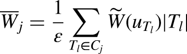
For all tets $T$ in the tesselation, compute the average integral

$$u_T=\frac{1}{|T|}{\int }_{T}u\mathrm{d}x$$

For each edge $e=e(T_1,T_2)$ in ${\mathrm{\Gamma }}_h$ corresponding to two adjacent tets $T_1$ and $T_2$ (i.e. tets sharing a common face), compute its weight as

$$w_e=\frac{F(u_{T_1})+F(u_{T_2})}{2}\cdot \frac{\mathrm{diam}(T_1)+\mathrm{diam}(T_2)}{2}$$

The second factor can be replaced by a generic grid length scale $h$ if the tets are sufficiently uniform. We refer to the associated distance as $d^{{\mathrm{\Gamma }}_h(u)}$ to emphasize the dependence of the distance (but not graph) on $u$ .

Create a list $I$ of all interface elements, that is all tets such that

$$u_T\in [\alpha ,\beta ]$$

Separate the elements in $I$ into connected components $\{C_j{\}}_{j=1}^M$ , where two tets $T_1,T_2\in I$ belong to the same component if $d^{{\mathrm{\Gamma }}_h(u)}(T_1,T_2)=0$ . If there is only one connected component, the algorithm can be terminated here as our approximations of both ${\mathcal{C}}_{\epsilon }$ and its variation vanish.

For $j\in \{1,\dots ,M\}$ calculate

$${\overline{W}}_j=\frac{1}{\epsilon }\sum _{T_l\in C_j}\tilde{W}(u_{T_l})|T_l|$$

For $i,j\in \{1,\dots ,M\}$ , $i\ne j$ calculate the component distances ${\overline{d}}_{ij}={\mathrm{dist}}^{{\mathrm{\Gamma }}_h(u)}(C_i,C_j)$ as well as the shortest connecting paths between components ${\overline{\gamma }}_{ij}=\{T_0^{ij},T_1^{ij},\dots ,T_{L(i,j)}^{ij}\}$ , $T_0^{ij}\in C_i$ , $T_{L(i,j)}^{ij}\in C_j$ .

The distance ${\mathrm{dist}}^{{\mathrm{\Gamma }}_h(u)}(C_i,C_j)$ is computed as $d^{{\mathrm{\Gamma }}_h(u)}(T_i,T_j)$ - for any two tets $T_i\in C_i$ and $T_j\in C_j$ . The exact choice of $T_i$ and $T_j$ is immaterial, since the distance between two elements in the same component is exactly zero. For any other pair $T_i^{\prime }\in C_i,T_j^{\prime }\in C_j$ we therefore have

$$d^{{\mathrm{\Gamma }}_h(u)}(T_i^{\prime },T_j^{\prime })\le d^{{\mathrm{\Gamma }}_h(u)}(T_i^{\prime },T_i)+d^{{\mathrm{\Gamma }}_h(u)}(T_i,T_j)+d^{{\mathrm{\Gamma }}_h(u)}(T_j^{\prime },T_j^{\prime })=d^{{\mathrm{\Gamma }}_h(u)}(T_i,T_j)$$

by the triangle inequality. The inverse inequality and invariance to choice of elements follow by exchanging the roles of $T_i,T_i^{\prime }$ and $T_j,T_j^{\prime }$ .

These computations can be performed using a variant of Dijkstra’s algorithm on ${\mathrm{\Gamma }}_h$ , which keeps track of the preceding tet in a shortest connecting path, see Dijkstra ¹² and Benmansour et al. ¹¹

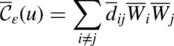
The approximate topological energy can now be computed as

$${\overline{\mathcal{C}}}_{\epsilon }(u)=\sum _{i\ne j}{\overline{d}}_{ij}{\overline{W}}_i{\overline{W}}_j$$

We note that, compared to the original double integral term, this is a major simplification, which is due to the specific choice of $F$ vanishing identically on the support of $\tilde{W}$ .

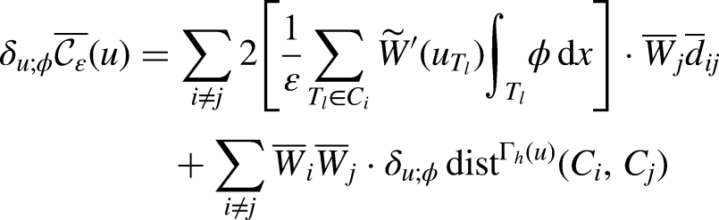
Our discrete approximation of the variation of ${\overline{\mathcal{C}}}_{\epsilon }$ with respect to a finite-element basis function $\varphi$ is then given by

$$\begin{array}{rl}{\delta }_{u;\varphi }\overline{{\mathcal{C}}_{\epsilon }}(u)& =\sum _{i\ne j}2[\frac{1}{\epsilon }\sum _{T_l\in C_i}{\tilde{W}}^{\prime }(u_{T_l}){\int }_{T_l}\varphi \mathrm{d}x]\cdot {\overline{W}}_j{\overline{d}}_{ij}\\ & +\sum _{i\ne j}{\overline{W}}_i{\overline{W}}_j\cdot {\delta }_{u;\varphi }{\mathrm{dist}}^{{\mathrm{\Gamma }}_h(u)}(C_i,C_j)\end{array}$$

where ${\delta }_{u;\varphi }{\mathrm{dist}}^{{\mathrm{\Gamma }}_h(u)}(C_i,C_j)={\delta }_{u;\varphi }{d}^{{\mathrm{\Gamma }}_h(u)}(T_i,T_j)$ for any $T_i\in C_i$ , $T_j\in C_j$ is given by (4).

This algorithm can be added to a given finite-element implementation. We may compute the time step from $u^k$ to $u^{k+1}$ with any scheme

$$\epsilon ⟨u_{k+1}-u_k,\varphi {⟩}_{L^2}=\tau [\mathrm{\Phi }(u_{k+1},u_k;\varphi )-\frac{1}{\epsilon }{\delta }_{u;\varphi }\overline{{\mathcal{C}}_{\epsilon }}(u)]$$

that treats the topological term explicitly. Here $\tau$ is the time-step size and $\mathrm{\Phi }$ is an explicit, implicit or mixed approximation of the variation $-\delta {\mathcal{F}}_{\epsilon }$ . As mentioned in Remark 1, in practical application, it has been proven useful to use the sum of two functionals of type ${\mathcal{C}}_{\epsilon }$ : one, ${\mathcal{C}}_{\epsilon }^{+}$ , to keep the portion of the interface close to $+1$ connected (i.e. with ${\alpha }^{+}$ and ${\beta }^{+}$ close to $+1$ ) and one, ${\mathcal{C}}_{\epsilon }^{-}$ to keep the portion of the interface close to $-1$ connected (i.e. with ${\alpha }^{-}$ and ${\beta }^{-}$ close to $-1$ ).

Remark 2

The high computational efficiency of our algorithm is due to step (7), as in practice this sum is only a sum of $<10$ components. This is the reason for discretizing the geodesic distance in the specific form of equation (4). Transport-based schemes, for example, proposed in Chambolle et al. ⁵ thus seem not suitable here.

Numerical results

We compare the discrete gradient flow (1) of ${\mathcal{F}}_{\epsilon }+\frac{a}{\epsilon }({\mathcal{C}}_{\epsilon }^{+}+{\mathcal{C}}_{\epsilon }^{-})$ , where ${\mathcal{F}}_{\epsilon }$ is given by (2) and either $a=0$ or $a=6.0\times {10}^1$ . The parameters in the simulation are $\epsilon =0.03$ , $\lambda =0.1$ , and $H_0=6$ .

Topological constraint

As mentioned at the end of section ‘The algorithm’, we implement the connectedness constraint using the sum of two functionals of type ${\mathcal{C}}_{\epsilon }$ , in this specific case ${\mathcal{C}}_{\epsilon }^{+}$ with $\alpha ={\alpha }^{+}=0.85$ , $\beta ={\beta }^{+}=0.95$ (in order to keep the part of the transition layer close to the phase $u=+1$ connected) and ${\mathcal{C}}_{\epsilon }^{-}$ one with $\alpha ={\alpha }^{-}=-0.95$ , $\beta ={\beta }^{-}=-0.85$ (in order to keep the part of the transition layer close to the phase $u=-1$ connected). We then write (with some abuse of notation) from now on ${\mathcal{C}}_{\epsilon }={\mathcal{C}}_{\epsilon }^{+}+{\mathcal{C}}_{\epsilon }^{-}$ .

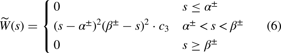
The functions $F$ and $\tilde{W}$ in ${\mathcal{C}}_{\epsilon }^{\pm }$ are given by

$$\begin{array}{rl}F(s)& =\{\begin{array}{cc}(s-\alpha {)}^2\cdot c_1& s<{\alpha }^{\pm }\\ 0& {\alpha }^{\pm }\le s\le {\beta }^{\pm }\\ ({\beta }^{\pm }-s{)}^2\cdot c_2& s>{\beta }^{\pm }\end{array}\end{array}$$

(5)

and

$$\begin{array}{rl}\tilde{W}(s)& =\{\begin{array}{cc}0& s\le {\alpha }^{\pm }\\ (s-{\alpha }^{\pm }{)}^2({\beta }^{\pm }-s{)}^2\cdot c_3& {\alpha }^{\pm }<s<{\beta }^{\pm }\\ 0& s\ge {\beta }^{\pm }\end{array}\end{array}$$

(6)

respectively, with $c_1$ , $c_2$ chosen such that $F(-1)=F(+1)=1$ and $c_3$ such that ${\int }_{-\mathrm{\infty }}^{\mathrm{\infty }}\tilde{W}(s)\mathrm{d}s=1$ .

The choices of parameters can be motivated heuristically. Fix $0<\alpha <\beta$ . We picture $u$ as a function with a steep transition layer of width on the order of $\epsilon$ which separates domains $\{u>\beta \}$ and $\{u<-\beta \}$ . As the surface $\mathrm{\Sigma }=\{u=0\}$ separates into two components ${\mathrm{\Sigma }}_1$ and ${\mathrm{\Sigma }}_2$ , one of the level sets ${\mathrm{\Sigma }}^{+}=\{u=(\alpha +\beta )/2\}$ and ${\mathrm{\Sigma }}^{-}=\{u=-(\alpha +\beta )/2\}$ must already be disconnected. In fact, since $u$ changes on a length scale $\epsilon$ , there exist two connected components ${\mathrm{\Sigma }}_1^{\pm },{\mathrm{\Sigma }}_2^{\pm }$ of at least one of the surfaces ${\mathrm{\Sigma }}^{\pm }$ such that

$${\mathrm{dist}}^{F(u)}({\mathrm{\Sigma }}_1^{\pm },{\mathrm{\Sigma }}_2^{\pm })\ge \overline{c}\epsilon$$

for some $\overline{c}$ which depends on the weight function $F$ and $|\alpha |$ as a measure how close ${\mathrm{\Sigma }}_{\pm }$ can be to $\mathrm{\Sigma }$ (compare Figure 4). The topological energy behaves roughly as

$${\mathcal{C}}_{\epsilon }(u)={\mathcal{C}}_{\epsilon }^{+}(u)+{\mathcal{C}}_{\epsilon }^{-}(u)\ge 2\left|{\mathrm{\Sigma }}_1^{\pm }\right|\cdot \left|{\mathrm{\Sigma }}_2^{\pm }\right|\cdot {\mathrm{dist}}^{F(u)}({\mathrm{\Sigma }}_1^{\pm },{\mathrm{\Sigma }}_2^{\pm })\ge |{\mathrm{\Sigma }}_1|\cdot |{\mathrm{\Sigma }}_2|\cdot \overline{c}\epsilon ,$$

since ${\int }_{\alpha }^{\beta }\tilde{W}(u)\mathrm{d}u=1$ . Depending on the magnitude of penalty parameter $a$ , the topological energy can therefore prevent ‘big’ pieces from disconnecting from $\mathrm{\Sigma }$ . Breaking off small pieces, on the other hand, is energetically unfavourable since every connected component has a minimum curvature energy

$${\int }_{\mathrm{\Sigma }}|H{|}^2\mathrm{d}A\ge {\int }_{S^2}|H{|}^2\mathrm{d}A=16\pi ,$$

see, for example, Dondl and Wojtowytsch. ¹⁰ If $H_0\ne 0$ , the same can be noted for very small surfaces, where $|H|\gg |H_0|$ on average. It is therefore almost always energetically favourable to absorb small amounts of the excess area into a global deformation rather than creating a new connected component for it.

Figure 4.

The figures show the sets $\{-0.95<u_T<-0.85\}$ (in blue) and $\{0.85<u_T<0.95\}$ (in red) as well as the zero-level set of $u$ (in grey), cut open for visibility. The picture on the left is taken just before the start of disconnectedness of either the blue or the red set. The image on the right shows the state after connectedness of the zero-level set of $u$ was lost (in the simulation without disconnectedness penalty). Clearly, disconnectedness of $\{u=0\}$ implies disconnectedness of $\{0.85<u_T<0.95\}$ here, thus there are two connected components of this set. Their connecting geodesic is shown in gold. The functional ${\mathcal{C}}_{\epsilon }$ is zero in the left image (as there is only one connected component of $\{-0.95<u_T<-0.85\}$ and $\{0.85<u_T<0.95\}$ ). It is non-zero in the right image, as there are two connected components of $\{0.85<u_T<0.95\}$ – the penalization would thus prevent this from occurring.

The parameters then can be chosen according to the following requirements:

$1/2<{\alpha }^{+}<{\beta }^{+}<1$ in order to bound $\overline{c}$ away from zero, as $\overline{c}$ is increasing with ${\alpha }^{+}$ and to ensure that $u^{-1}({\alpha }^{+},{\beta }^{+})$ is a meaningful approximation of the interface. These constants can be chosen independently of $\epsilon$ .

$|{\beta }^{+}-{\alpha }^{+}|$ is large enough compared to $h$ that ${\mathcal{C}}_{\epsilon }$ can be evaluated in a stable fashion. It seems to suffice to require that ${\varphi }^{-1}({\beta }^{+})-{\varphi }^{-1}({\alpha }^{+})\ge 4\frac{h}{\epsilon }$ , where $\varphi (t)=\tanh (t/\sqrt{2})$ is the optimal profile from Figure 1.

The strength of the penalization $a$ is chosen empirically to prevent topological transitions, the value will depend on the amount of energy gained by a pinch-off. By the heuristics above, the minimal weight which prevents the loss of connectedness does not depend on $\epsilon >0$ in a critical way, but may depend on $H_0$ and the initial condition of a given simulation.

Due to the condition $\int \tilde{W}(u)=1$ , the constant $a>0$ does not strongly depend on the choice of ${\alpha }^{+},{\beta }^{+}$ if $({\alpha }^{+},{\beta }^{+})$ is bounded away from $0$ .

It is simplest to set ${\alpha }^{-}=-{\beta }^{+},{\beta }^{-}=-{\alpha }^{+}$ . We note that any choice $a>0$ prevents the loss of connectedness on mesoscopic or macroscopic scales $\gg \epsilon$ .

From a computational standpoint, it is advisable to choose $a$ as small as possible, since the gradient of the topological term acts on $u$ in a somewhat discontinuous fashion as it concentrates on low-dimensional objects. If $a$ is taken too large, the time-step size must become small, even if the curvature energy is treated in an implicit fashion. For more numerical experiments illuminating see also Dondl et al.^1,2

Finite-element simulations

The computational domain is a discretization of the 3D unit ball by $\sim 1.6\times {10}^6$ tetrahedral $P1$ finite elements. Our time-stepping algorithm is a simple first-order fully implicit Euler scheme coupled to an explicit treatment of ${\mathcal{C}}_{\epsilon }$ as described in section ‘The algorithm’. The time step size is given by $\tau =5\times {10}^{-7}$ (with a smaller time step $\tau =1\times {10}^{-8}$ for the first several hundred time steps during the fast convergence to the optimal profile). The higher spatial gradient in the energy is treated using a Ciarlet–Raviart–Monk mixed formulation^13,14 with clamped boundary conditions $u=-1$ on $\mathrm{\partial }\mathrm{\Omega }$ and $\mathrm{\partial }u/\mathrm{\partial }n=0$ on $\mathrm{\partial }\mathrm{\Omega }$ and we note that on our convex domain this variational crime is only a misdemeanor. ¹⁵

The initial condition is an approximation of the characteristic function of an ellipsoid with principle axes $0.7$ , $0.3$ , and $0.3$ . As seen in Figure 2, in the simulation of the case $a=0$ , without topological constraint, the surface undergoes a pinch-off and the final steady state is given by two spheres of radius $\approx \frac{1}{6}$ . A similar result of pinch-off was observed in Du et al. ^{16 1}

Figure 2.

Simulation results for the geometric flow without connectedness penalty. Shown are the initial condition (after some relaxation) at time $t=1\times {10}^{-5}$ , an intermediate configuration just before pinch-off at $t=3.0\times {10}^{-4}$ and the final state which was reached at $t=5.0\times {10}^{-4}$ . The colour indicates the mean curvature, the image shows the zero-level set of the phase-field function $u$ .

The simulation results for the case $a=6.0\times {10}^1$ , that is, including the topological constraint, are shown in Figure 3. One can clearly see that the pinch-off into two components has been suppressed and a dumbbell-like shape is the final result. We conjecture that this shape is in fact a stationary point of the energy as no further motion was observed in the simulation even on a longer time scale.

Figure 3.

Simulation results for the geometric flow with connectedness penalty. The first two images are the same as in Figure 2, since no disconnectedness had occurred yet. The final state in the third image was reached at $t=4.0\times {10}^{-4}$ .

We note that at the pinch-off, the function $u$ dips below $0.85$ and thus the start of the interface becoming disconnected is detected by the algorithm. For an illustration see Figure 4.

The equilibrium was reached in $\sim$ 9 h of wall-time using 8 cores of a computer server equipped with two Intel Xeon E5-2690 v4 processors. We note that the central processing unit (CPU)-time spent computing the topological constraint is negligible (<0.1% of the total CPU-time) – the only computational down-side may thus be the aforementioned restriction on the time-step size due to the necessary explicit treatment of ${\mathcal{C}}_{\epsilon }$ . The implicit treatment of ${\mathcal{C}}_{\epsilon }$ is analytically questionable due to the lack of regularity of ${\mathcal{C}}_{\epsilon }$ .