In this paper, a fractional order avian-human influenza epidemic model with logistic growth for avian population is investigated. The dynamical behavior of this model is discussed. We first establish the existence, uniqueness, non-negativity and positive invariance of the solution. Then we analyze the existence of various equilibrium points, and some sufficient conditions are derived to ensure the global asymptotic stability of the disease free equilibrium point and endemic equilibrium point. Finally, we take some numerical simulations to validate the analytical results.
Avian influenza is an infectious disease of birds caused by type A strains of the influenza virus. Most avian influenza viruses do not cause disease in humans. However, some can infect humans and cause disease. Influenza A virus subtype H5N1 is a highly pathogenic avian influenza virus, which was first detected in 1996 in geese in China and first detected in humans in 1997 during a poultry outbreak in Hong Kong.1 Differing from H5N1, the H7N9 virus is classified as a low pathogenicity avian influenza virus.2 However, the virus can infect humans and most of the reported cases of human H7N9 infection have resulted in severe respiratory illness.3 So it is important for us to take effective measure to prevent the avian influenza and limit its damage at the minimum.
Mathematical modeling represents an important tool for analyzing the epidemiological characteristics of infectious diseases and can provide useful control measures. Various of mathematical compartmental models have been introduced to study the mechanism of the spread of avian influenza.1,4–8 However, most of these studies focused on an integer-order compartmental epidemic model as a key tool for their investigation. In recent years, it has frequently been observed in many areas of engineering, physics, life sciences, and elsewhere that models based on fractional order derivatives can provide better agreement between measured and simulated data than classical models based on integer order derivatives9,10 and the references therein.
In fact, fractional-order differential equations are naturally related to systems with memory which exists in most biological systems, and they have close relations to fractals which are abundant in biological systems. In recent past, fractional order differential equations have been used in several biological systems to explore the underlying dynamics. In Diethelm,11 Diethelm proposed a nonlinear fractional order differential equation model for the simulation of the dynamics of a dengue fever outbreak. Sardar et al.12 proposed two mathematical models to study the spread of a common single strain mosquito-transmitted diseases. Some fractional order models for HIV infection were studied in literature.13,14 In Gonzalez-Parra et al.,15 the authors proposed a SEIR epidemic fractional differential model to explain and understand the outbreaks of influenza A(H1N1). Li et al.16 investigated a fractional-order single-species model, which is composed of patches connected by diffusion. A homogeneous-mixing population fractional model for human immunodeficiency virus (HIV) transmission was proposed in Huo et al.17 A nonlinear fractional order epidemic model was proposed in Ye et al.18 to investigate the spreading dynamical behavior of the avian influenza. Also we refer the interested reader in fractional biological systems19–22 and the references therein for some other recent works in the subject. However, to the best of our knowledge, to this day, less work has investigated the dynamic behavior of fractional-order avian-human influenza model.
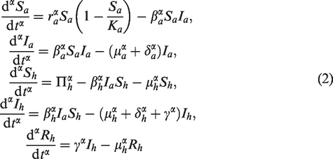
In this paper, we consider the following fractional-order avian-human influenza model:
with denoting the left-sided Caputo fractional derivative of order following Podlubny,23 defined as
where is the Gamma function. In model (1), and are the population densities or numbers of susceptible and infective avian population, respectively; and are the population densities or numbers of susceptible, infective and recovered/removed human population, respectively; ra and Ka are the intrinsic growth rate and maximal carrying capacity of the avian population, respectively; βa is the transmission rate from infective avian to susceptible avian; μa and δa are the natural death rate and disease death rate of the avian population, respectively. Πh represents all new recruitments and newborns of the human population; βh is the transmission rate from the infective avian to the susceptible human, μh is the natural death rate of the human population; δh is the disease related rate of the infected human population; γ is the recovery rate of the infective human. All parameters are assumed to be positive from biological point of view. The case of integer order model, i.e., the counterpart with α = 1 of (1) has been investigated by Liu et al.24
A simple dimensional analysis of model (1) shows that the left-hand side of the system (1) has dimension (time) whereas the right-hand side dimension is (time)–1. This dimension mismatch of the system (1) can be mathematically corrected using the procedure described in Diethelm.11 A corrected form corresponding to model (1) is written as
In this paper we will investigate the above system, subject to an initial condition given at t = t0. The remaining of this paper is organized as follows. In the next section, we derive the well-posedness of the problem. The dynamical behavior of the model are presented in ‘Dynamical behavior’ section. Finally, we present some numerical simulations in the penultimate section to verify our theoretical results. Some concluding remarks are given at the end of the paper.
Well-posedness
In this section, we will prove the existence, uniqueness, non-negativity and boundedness of the solutions. We first introduce some basic results.
Preliminaries
Lemma 2.1(Generalized mean value theorem25) Suppose thatandwiththen we have
where
Lemma 2.220Let u(t) be a continuous function onand satisfywhereandis the initial time. Then, its solution has the form
is the Mittag–Leffler function with parameter α.
Lemma 2.319Letbe a continuous and derivable function. Then, for any time instant,
where
Existence and uniqueness
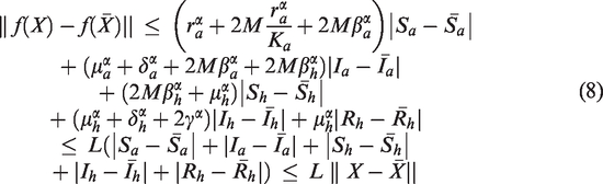
Theorem 2.1The system (2) possesses a unique continuous solution on, whereand M is sufficiently large.
Proof. We denote and . Consider a mapping and
For any , it follows from (3) that
Note that
Furthermore, we obtain that
Similarly, we get
Plugging (5), (6) and (7) into (4), we have
where
Thus f(X) satisfies Lipschitz condition with respect to X, and it follows from the existence and uniqueness theorem (Theorem 3.4 in Podlubny23) that there exists a unique solution X(t) of the system (2) with the initial condition . □
Nonnegativity and boundedness
Considering biological significance of the problem, we are only interested in solutions that are nonnegative and bounded. Denote and
Theorem 2.2All solutions of the system (2) that start inare nonnegative and uniformly bounded.
Proof. Firstly, we prove that the solutions which start in are non-negative. Assuming for t = 0, we first prove that for all . Let us suppose that is not true. Then, there exists a such that for at t = t1 and for From the first equation of (2), we have
According to Lemma 2.1, we have which contradicts the fact , i.e., for Therefore, we have . Using similar arguments, we can prove that are all non-negative for . Next, we show that all solutions of system (2) that start in are uniformly bounded.
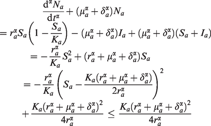
Adding the first two equations of (2) and adding last three equations of (2), we get two fractional order differential equations representing the total avian and human population as follows:
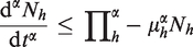
and
where and Then from (9) we have
Applying Lemma 2.2, one gets
Thus, as .
Since , we get from (10) that
Again by Lemma 2.2, we have
Therefore, all the solutions of system (2) which start in are confined to the region
with any . □
We will consider the stability of the equilibria of system (2) and its qualitative behaviors in the following sections.
Dynamical behavior
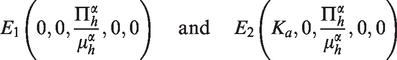
From (2), we can deduce two disease-free equilibria given by
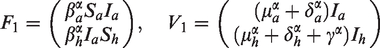
Following the definition and computation procedure in Diekmann et al.26 and van den Driessche and Watmough,27 we can rewrite system (2) as follows:
where and
Let
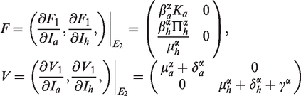
then
and
Hence, we derive the basic reproduction number as follows
where ρ denotes the spectral radius or largest eigenvalue of .
If , we can also derive a unique endemic equilibrium given by where
Before analyzing the dynamical behavior of the full model (2), we study the dynamical behavior of the avian-only subsystem.
Analysis of the avian-only subsystem
In this subsection, we will consider the dynamics of fractional order avian-only subsystem, which is independent of the human system, as follows:
The avian-only subsystem (14) always has two disease-free equilibria given by and . If , the system also has a unique endemic equilibrium given by .
Lemma 3.1(i) The disease-free equilibriumof (14) is always unstable; (ii) If, then the disease-free equilibriumof (14) is locally asymptotically stable, otherwise it is unstable. (iii) If, the endemic equilibriumof (14) is locally asymptotically stable.
Proof. (i) The Jacobian matrix of system (14) evaluated at is given by
By solving the characteristic equation , with I2 being the unit matrix, we get the following eigenvalues
Note that and . Since the first eigenvalue λ1 does not satisfy for all therefore is always unstable.
(ii) The Jacobian matrix is computed as
The corresponding eigenvalues are
Here, two cases arise depending on whether or .
Case 1. If , then we can see that . Therefore, the equilibrium is locally asymptotically stable.
Case 2. If , then it is easy to see that . In this case, is unstable.
(iii) The Jacobian matrix is computed as
The corresponding characteristic equation becomes
Since and if , all eigenvalues have negative real parts. Therefore, . Hence, the equilibrium is locally asymptotically stable. □
Lemma 3.2If, then the disease-free equilibriumof (14) is globally asymptotically stable.
Proof. We consider the following positive definite function given by
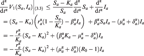
Here, V1 is a C1 function such that for all values of and only at . Calculating the α order derivative of along the solution of system (14), it follows from Lemma 2.3 that
Note that if then for all , and at . Therefore, the only invariant set on which is the singleton . Then using Lemma 4.6 in Huo et al.17 which generalizes the integer-order LaSalle Invariance Principle to fractional-order system, it follows that every nonnegative solution tends to when . Thus, is globally asymptotically stable if . □
Lemma 3.3If, then the endemic equilibriumof (14) is globally asymptotically stable.
Proof. Since is the equilibrium point of system (14), we have
Next, the global asymptotic stability of the equilibrium point of system (14) will be demonstrated.
Let us define the Lyapunov function as
Here, V2 is a C1 function such that for all values of and only at . Calculating the α order derivative of along the solution of system (14), it follows from Lemma 2.3 that
Clearly, for all , and implies that . In fact, implies that . When , from the first equation of system (14), we obtain
it follows from the first equation of (15) and (16) that . That is, implies that . Therefore, the only invariant set on which is the singleton . By Lemma 4.6 in Huo et al.,17 it follows that the equilibrium point of (14) is globally asymptotically stable if . This completes the proof of Lemma 3.3.
Analysis of the full system
Since the first four equations of system (2) are independent of the variable Rh, we only need to analyze the dynamical behavior of the following equivalent reduced system
System (17) always has two disease-free equilibria given by and If , then system (17) also has a unique endemic equilibrium given by .
Lemma 3.4(i) The disease-free equilibriumis always unstable. (ii) If, then the disease-free equilibriumis locally asymptotically stable, otherwise it is unstable. (iii) If, then the disease-free equilibriumis unstable and the endemic equilibriumis locally asymptotically stable.
Proof. The characteristic equation of the Jacobian matrix at an arbitrary equilibrium takes the form
If , the eigenvalues are and Note that , and . Since the third eigenvalue λ3 does not satisfy for all , therefore is always unstable.
If , we get from (18) that the eigenvalues are , and . If , then we get that Therefore, the equilibrium is locally asymptotically stable. If , then it is easy to see that , hence is unstable.
If and , by plugging (13) into (18), one gets
It is easy to see that are two of the eigenvalues. The remaining two eigenvalues, λ3 and λ4, are the roots of the equation
Since and if , all eigenvalues have negative real parts. Therefore, . Hence, the equilibrium is locally asymptotically stable. □
Theorem 3.1If, then the disease-free equilibriumof the full reduced system (17) is globally asymptotically stable.
Proof. According to Lemma 3.2, the disease-free equilibrium of (14) is globally asymptotically stable if . To prove the global stability of , we only need to consider system (17) with the avian components already at the disease-free steady state, given by
Clearly, we can obtain that if . Hence, the disease-free equilibrium is globally asymptotically stable. □
Theorem 3.2If, then the endemic equilibriumof the full reduced system (17) is globally asymptotically stable.
Proof. By Lemma 3.3, the endemic equilibrium of (14) is globally asymptotically stable if . To prove the global stability of the equilibrium , we only need to consider system (17) with the avian components already at the endemic steady state, given by
We can easily deduce that subsystem (22) has a unique positive equilibrium which is locally asymptotically stable.
To prove the global stability of the positive equilibrium of subsystem (22), we choose a Lyapunov function as follows
Here, V3 is a C1 function such that for all values of and only at . Calculating the α order derivative of along the solution of system (22), it follows from Lemma 2.3 that
Since is the equilibrium point of system (22), we have
which leads to
It follows that
and
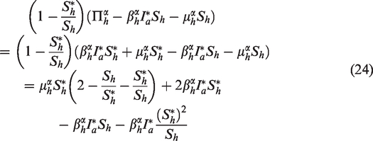
Plugging (24) and (25) into (23), we obtain
Since the arithmetic mean exceeds the geometric mean, we have
Hence, for all , and implies that . Again, by Lemma 4.6 in Huo et al.,17 it follows that and as . Therefore, the endemic equilibrium of the full system (17) is globally asymptotically stable. □
Now we can state our results for the full avian-human model (2).
Theorem 3.3(i) The disease-free equilibrium E1 of model (2) is always unstable; (ii) If, then the disease-free equilibrium E2 of model (2) is globally asymptotically stable. (iii) If, then then the disease-free equilibrium E2 of model (2) is unstable but the endemic equilibrium E3 of model (2) is globally asymptotically stable.
Remark 3.1The above stability results we obtained for the fractional order model is also true for α = 1, which has been obtained by Liu et al.24
Numerical simulations
In this section, numerical simulations are provided to substantiate the theoretical results established in the previous section of this paper. In addition, we also show the effects of fractional order α on the stability of the equilibrium points, these numerical simulations are very important from biological point of view.
The existing numerical methods for fractional differential equations include finite difference, Galerkin finite element, spectral method and so on. The time stepping scheme employed in our simulations is the so-called order finite difference method, proposed by Lin and Xu 28 for the temporal discretization of the time fractional diffusion equation. It was proved by Lin and Xu that this scheme is unconditionally stable, and the convergence rate is of order, where is the order of the fractional derivative. In what follows, all the parameter values are chosen hypothetically due to the unavailability of real world data.
We consider the parameter values as and initial point .
In Figure 1, we plot the variation of the value of the reproduction number for different values of α. It is observed that as α is decreased from 1, R0 goes to values more than 1. This indicates that at an order there is a bifurcation from a disease-free equilibrium () to a stable endemic equilibrium () in the model. Thus, analytically, α is a bifurcation parameter of the model.
Variation of the reproduction number, R0, versus the order of the fractional derivative α.
Let The corresponding reproduction numbers are , respectively. Following Theorem 3.1, the disease-free equilibrium of (2) is stable. In Figure 2, we plot the solutions of the reduced system (17) with different values of α. It shows that all populations remain stable for all values of α though solutions reach to equilibrium value more slowly for larger value of α.
Dynamics of model (17) for .
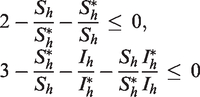
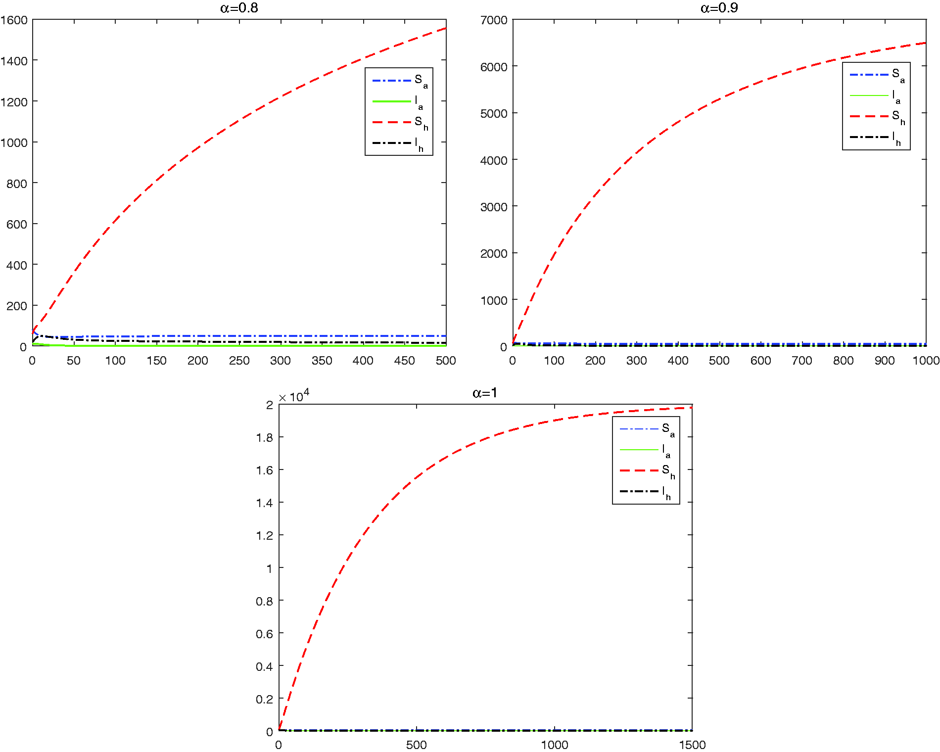
Now we choose . The corresponding reproduction numbers are 4.5080, 2.9289, 1.9008, respectively. Following Theorem 3.2, the endemic equilibrium of (2) is stable. In Figures 3to 5, we report the dynamics of model (17) for . As expected, the disease is endemic, since all the solutions of model (17) approach to the endemic equilibrium .
Global asymptotic stability of the endemic equilibrium point for . Upper: Time series of ; Lower: phase portrait of the avian system (left) and the reduced human system (right) with different initial value.
Global asymptotic stability of the endemic equilibrium point for . Upper: Time series of ; Lower: phase portrait of the avian system (left) and the reduced human system (right) with different initial value.
Global asymptotic stability of the endemic equilibrium point for . Upper: Time series of ; Lower: phase portrait of the avian system (left) and the reduced human system (right) with different initial value.
In Figures 6 and 7, we plot the variation of the avian infective individuals and the human infective individuals for different values ν. One can see from Figures 6 and 7 that both Ia and Ih tends to a stationary state over a longer period of time with decreasing the value of α.
Numbers of avian infective individuals for different values α.
Numbers of human infective individuals for different values α.
Concluding remarks
In this paper, we have proposed a fractional order avian-human influenza epidemic model with logistic growth for avian population. We prove that the solution of the model exists uniquely and all solutions remain positive and bounded whenever they start with positive initial value, thus justifying the well-posedness of a biological model. We show that our system contains three equilibrium points. The trivial equilibrium point is always unstable, implying that all populations can not go to extinction simultaneously. The disease free equilibrium is locally and globally asymptotically stable if , and the endemic equilibrium is locally asymptotically and globally stable if Our numerical results show that solutions of fractional order system converge to the respective equilibrium more slowly as the order of the differential equation becomes smaller.
Footnotes
Declaration of Conflicting Interests
The author(s) declared no potential conflicts of interest with respect to the research, authorship, and/or publication of this article.
Funding
The author(s) disclosed receipt of the following financial support for the research, authorship, and/or publication of this article: Xingyang Ye was partially supported by the Scientific Research Foundation of Jimei University of China (Grants ZP2020062 and ZP2020054), Foundation of Fujian Provincial department of education (Grants JAT190326 and JT180262), Natural Science Foundation of Fujian Province of China (Grants 2018J01418). Shimin Lin was partially supported by National NSF of China (Grant 11901237). Chuanju Xu was partially supported by NSFC grant 11971408, NNW2018-ZT4A06 project, and NSFC/ANR joint program 51661135011/ANR-16-CE40-0026-01.
ORCID iDs
Xingyang Ye
Chuanju Xu
References
1.
IwamiSTakeuchiYLiuXN.Avian-human influenza epidemic model. Math Biosci2007;
207: 1–25.
2.
Pantin-JackwoodMJMillerPJSpackmanE, et al.
Role of poultry in the spread of novel H7N9 influenza virus in China. J Virol2014;
88: 5381–5390.
3.
LiQZhouLZhouM, et al.
Epidemiology of human infections with avian influenza A(H7N9) virus in China. N Engl J Med2014;
370: 520–532.
4.
KimKILinZGZhangL.Avian-human influenza epidemic model with diffusion. Nonlinear Anal Real World Appl2010;
11: 313–322.
5.
SamantaGP.Permanence and extinction for a nonautonomous avian-human influenza epidemic model with distributed time delay. Math Comput Modelling2010;
52: 1794–1811.
6.
TangQLGeJLinZG.An SEI-SI avian-human influenza model with diffusion and nonlocal delay. Appl Math Comput2014;
247: 753–761.
ZhangXH.Global dynamics of a stochastic avian-human influenza epidemic model with logistic growth for avian population. Nonlinear Dynam2017;
90: 2331–2343.
9.
BaleanuDDiethelmKScalasE, et al.Fractional calculus: models and numerical methods.
Singapore:
World Scientific, 2012.
10.
DiethelmK.The analysis of fractional differential equations.
Berlin:
Springer-Verlag, 2010.
11.
DiethelmK.A fractional calculus based model for the simulation of an outbreak of dengue fever. Nonlinear Dyn2013;
71: 613–619.
12.
SardarTRanaSBhattacharyaS, et al.
A generic model for a single strain mosquito-transmitted disease with memory on the host and the vector. Math Biosci2015;
263: 18–36.
13.
DingYSYeHP.A fractional-order differential equation model of HIV infection of CD4+ T-cells. Math Comput Model2009;
50: 386–392.
14.
PintoCMACarvalhoARM.A latency fractional order model for HIV dynamics. J Comput Appl Math2017;
312: 240–256.
15.
Gonzalez-ParraGArenasAJChen-CharpentierBM.A fractional order epidemic model for the simulation of outbreaks of influenza A(H1N1). Math Methods Appl Sci2014;
37: 2218–2226.
16.
LiHLZhangLHuC, et al.
Dynamic analysis of a fractional-order single-species model with diffusion. Nonlinear Anal Model Control2017;
22: 303–316.
17.
HuoJJZhaoHYZhuLH.The effect of vaccines on backward bifurcation in a fractional order HIV model. Nonlinear Anal Real World Appl2015;
26: 289–305.
18.
YeX and XuC.A Fractional Order Epidemic Model and Simulation for Avian Influenza Dynamics. Math Meth Appl Sci2019;
42: 4765–4779.
19.
Vargas-De-LeoNC,
Volterra-type Lyapunov functions for fractional-order epidemic systems. Commun Nonlinear Sci Numer Simul2015;
24: 75–85.
20.
LiHLZhangLHuC, et al.
Dynamical analysis of a fractional-order predator-prey model incorporating a prey refuge. J Appl Math Comput2017;
54: 435–449.
21.
SaeedianMKhalighiMAzimi-TafreshiN, et al.
Memory effects on epidemic evolution: the susceptible-infected-recovered epidemic model. Phys Rev E2017;
95: 022409.
22.
MondalSLahiriABairagiN.Analysis of a fractional order eco-epidemiological model with prey infection and type 2 functional response. Math Methods Appl Sci2017;
40: 6776–6789.
23.
PodlubnyI.Fractional differential equations.
New York:
Acad. Press, 1999.
24.
LiuSRuanSZhangX.Nonlinear dynamics of avian influenza epidemic models. Math Biosci2017;
283: 118–135.
25.
OdibatZMShawagfehNT.Generalized Taylor’s formula. Appl Math Comput2007;
186: 286–293.
26.
DiekmannOHeesterbeekJAP.Mathematical epidemiology of infectious diseases: model building, analysis and interpretation.
New York:
Wiley, 2010.
27.
DriesschePWatmoughJ.Reproduction numbers and sub-threshold endemic equilibria for compartmental models of disease transmission. Math Biosci2002;
180: 29–48.
28.
LinY and XuC.Finite Difference/spectral Approximations for the Time-Fractional Diffusion Equation. Journal of Computational Physics2007;
225: 1533–1552.