Galerkin method with splines for total variation minimization

Abstract

Total variation smoothing methods have been proven to be very efficient at discriminating between structures (edges and textures) and noise in images. Recently, it was shown that such methods do not create new discontinuities and preserve the modulus of continuity of functions. In this paper, we propose a Galerkin–Ritz method to solve the Rudin–Osher–Fatemi image denoising model where smooth bivariate spline functions on triangulations are used as approximating spaces. Using the extension property of functions of bounded variation on Lipschitz domains, we construct a minimizing sequence of continuous bivariate spline functions of arbitrary degree, d, for the TV-L² energy functional and prove the convergence of the finite element solutions to the solution of the Rudin, Osher, and Fatemi model. Moreover, an iterative algorithm for computing spline minimizers is developed and the convergence of the algorithm is proved.

Introduction

A few decades ago, Rudin et al.¹ proposed a constrained total variation minimization method for image enhancement. Suppose you have an image f filled with artifacts and your goal is to reduce these artifacts and enhance the quality of your image while preserving the details of the image as much as possible. Assuming that the image f is a function defined on regular domain $\Omega \subset {\mathbb{R}}^2$ , Rudin, Osher and Fatemi’s (ROF) approach is to solve the following penalized total variation minimization problem

$$\underset{u\in L^{\text{2}}(\Omega )}{\text{arg} \text{min}}\lambda {\displaystyle {\int }_{\Omega }\text{|}}Du\mathrm{|+}\frac{\text{1}}{\text{2}}{\displaystyle {\int }_{\Omega }\text{|}}{u-f\text{|}}^{\text{2}}\text{d}x$$

(1)

where ${\int }_{\Omega }|Du|$ is the total variation of u, and λ is a positive parameter controlling the fidelity of the recovered image to the initial image f. From now on we will denote the total variation of a function u by

$$J(u):={\displaystyle {\int }_{\Omega }|}Du|$$

(2)

We shall refer to the minimization problem (equation (1)) as the ROF model, and denote its objective functional by

$$E_{\lambda }^f(u):=\lambda J(u)+\frac{1}{2}{\displaystyle {\int }_{\Omega }|}u-f{|}^2\text{d}x$$

(3)

Notice that a minimal condition for the ROF model to be defined is that the image f be a square integrable function over Ω in which case the domain of $E_{\lambda }^f(u)$ is $\mathit{BV}(\Omega )\cap L^2(\Omega )$ , where $\mathit{BV}(\Omega )$ stands for the space of functions of bounded variation over Ω.

The last decades witnessed excellent progress and exciting development regarding the analysis of the ROF model. The interested reader is referred to Chambolle et al. ² for a comprehensive introduction on this topic. Since the introduction of the model, much understanding is gained on the analytic properties of its solution (c.f. Caselles et al.,³ Allard,^4,5 and Caselles et al.⁶). For instance, it is known that, the solution of the model does not introduce new discontinuity compared to the input data. Specifically, it was proved in Caselles et al.⁶ that the jump set of the solution is always contained in the jump set of the input image; and if Caselles et al.³ f has modulus of continuity ω, then so does the minimizer of $E_{\lambda }^f(u)$ provided that Ω is convex. A concise outline of recent progress on the study of the properties of the continuous model can be found at Chambolle et al.⁷

On the computational side of the model, early algorithms were based on smooth approximations of the primal form of the variational problem (equation (1)) (c.f. Acar and Vogel⁸ and Chambolle and Lions⁹). Chambolle ¹⁰ first proposed a gradient descent algorithm that operated on the dual form of the original minimization problem. In addition, He proved that this algorithm converged to the exact solution of the discretized model (c.f. Chambolle^10,11). Much progress had since been made in the 2000s to develop highly accelerated first-order algorithms (c.f. Aujol and Dossal, ¹² Beck and Teboulle, ¹³ Beck,¹⁴ Combettes and Wajs, ¹⁵ Esser et al., ¹⁶ Goldstein and Osher,¹⁷ Zhu and Chan,¹⁸ and Zhu et al. ¹⁹ ) to solve the dual problem. See Chambolle and Pock²⁰ for a recent survey on such numerical methods. Independent of the aforementioned approaches, there is another class of combinatorial optimization methods that are very efficient and have been extensively studied by the computer vision community (c.f. Boykov et al.,²¹ Darbon and Sigelle,^22,23 and Goldfarb and Yin ²⁴ ). We note that in all aforementioned works, the discretization of the ROF model is always carried out on a fixed rectangular grid where finite difference schemes are convenient to compute the total variation. Error bound of such discretization was derived in Lai et al.²⁵ and Wang and Lucier. ²⁶

To the best of our knowledge, Dobson and Vogel²⁷ (Theorem 2.2, p. 1782) are among the first to investigate solving the total variation minimization problem with Galerkin schemes. They gave a sufficient condition for the convergence of a Galerkin scheme for the ROF model. However, they also observed that the said condition is easily achieved if the solution of the ROF model is sufficiently smooth and suggested that more research be done under less stringent regularity assumptions. Along this line of study, many well-developed methods in the theory of finite element method are applied to this problem (c.f. Lai and Messi, ²⁸ Matamba Messi, ²⁹ Bartels,^30,31 Bartels and Milicevic, ³² Chen and Tai, ³³ Feng and Prohl, ³⁴ Feng et al., ³⁵ Litvinov et al., ³⁶ Stamm and Wihler, ³⁶ Tian and Yuan, ³⁷ and Xu et al. ³⁸ ). It is worth noting that all these works employ either piecewise-constant or piecewise-linear finite elements. They also presume certain regularity conditions on the input data with the exception of Bartels’ work.

This paper addresses Dobson and Vogel’s question by constructing a convergent Galerkin scheme regardless of the regularity of the solution of the ROF model. The novelty of our method is we extend the conventional piecewise-linear finite-elements–based approach to bivariate spline element with arbitrary degree, and prove the convergence of the numerical scheme. We also propose a relaxation algorithm for solving the variation problem using bivariate splines. We note in numerical experiments that unlike other algorithms that use finite difference schemes, the spline algorithm that we propose does not show the notorious “staircase” effect. We also gain flexibility with the capability to select any polygonal region in an image for local treatment; this was not easy with algorithms that required rectangular patches when doing local denoising. Our method is also anticipating the day when we will be able to capture images with non-rectangular CCD devices.

The paper is structured as follows. The next section is devoted to the necessary mathematical preliminaries on functions of bounded variation and bivariate spline functions. In the Galerkin approximation with smooth splines section, we review relevant properties of the ROF model and prove the main result (Theorem 11) of this paper. We introduce an algorithm for approximating the terms of the spline minimizing sequence and prove its convergence in the Fixed point relaxation algorithm section. In the last section, we show the numerical evidence of its effectiveness at smoothing images.

Preliminary results

In this section and throughout the paper, the planar domain Ω is assumed polygonal, unless otherwise noted. We also remind the reader that by domain of ${\mathbb{R}}^2$ , we mean a connected open subset.

Functions of bounded variation

A function $u:\Omega \to \mathbb{R}$ is said to be of bounded variation if $u\in L^1(\Omega )$ and its total variation

$$J(u):=\sup \{{\displaystyle {\int }_{\Omega }u}\text{div}(\phi )\mathrm{d}x:\phi \in C_c^1(\Omega ,{\mathbb{R}}^2)$$

(4)

$$|\phi (x)|\le 1,\forall x\in \Omega \}$$

(5)

is finite. For example any function $u\in {\text{W}}^{1,1}(\Omega )$ is of bounded variation with total variation

$${\displaystyle {\int }_{\Omega }|}Du|={\displaystyle {\int }_{\Omega }|}\nabla u|\text{d}x$$

(6)

The set of functions of bounded variation, denoted $\mathit{BV}(\Omega )$ , is a Banach space for the norm

$$\left|\right|u|{|}_{\mathit{BV}}:=|\left|u\right|{|}_{L^1}+{\displaystyle {\int }_{\Omega }|}Du|$$

(7)

Furthermore, if $u\in \mathit{BV}(\Omega )$ , then its distributional derivative,⁴⁰ Du, is a finite vector-valued Radon measure on Ω, and the total variation of Du induces a Borel measure on Ω known as the total variation measure of u over Ω.

The following result asserts that a function u defined on a domain Ω of ${\mathbb{R}}^2$ with zero total variation must be constant. In particular, if $\Omega ={\mathbb{R}}^2$ , then the total variation is a norm on $\mathit{BV}({\mathbb{R}}^2)$ equivalent to the norm $\left|\right|·|{|}_{\mathit{BV}}$ defined in equation (7).

Theorem 1 (Poincaré Inequality^41,42). Suppose that Ω is a bounded Lipschitz domain of ${\mathbb{R}}^2$ . Then there exists a constant C depending only on Ω such that

$$\left|\right|u-u_{\Omega }|{|}_{L^2(\Omega )}\le C{\displaystyle {\int }_{\Omega }|}Du|,\forall u\in \mathit{BV}(\Omega )$$

(8)

where $u_{\Omega }=\frac{1}{\left|\Omega \right|}{\int }_{\Omega }u(x)\text{d}x$ is the average value of u over Ω. If $\Omega ={\mathbb{R}}^2$ , then there exists C > 0 such that for any compactly supported function $u\in \mathit{BV}({\mathbb{R}}^2)$

$$\left|\right|u|{|}_{L^2({\mathbb{R}}^2)}\le C{\displaystyle {\int }_{{\mathbb{R}}^2}|}Du|$$

(9)

Another property of functions of bounded variation that is central to our contribution in this work is the existence of an extension operator from $\mathit{BV}(\Omega )$ into $\mathit{BV}({\mathbb{R}}^2)$ that does not turn the boundary of Ω into a singular set for the total variation measure.

Theorem 2 ⁴¹ (Proposition 3.21, p. 131). Suppose that Ω is a bounded Lipschitz domain. Then for any bounded open set $A\subset {\mathbb{R}}^2$ such that Ω is relatively compact in A, there exists a bounded linear extension operator $T_A:\mathit{BV}(\Omega )\to \mathit{BV}({\mathbb{R}}^2)$ such that the following hold:

For any $u\in \mathit{BV}(\Omega ),\left|D{T}_{A}u\right|(\Gamma )=0$ and the support of T_Au is contained in A.

The restriction of T_A to $W^{1,1}(\Omega )$ is a bounded linear operator into $W^{1,1}({\mathbb{R}}^2)$ .

Proof. The proof is constructive and parallels the construction of an extension operator³⁹ from W′^1,1(Ω) to $W^{1,1}({\mathbb{R}}^2)$ using a partition of unity argument. The complete proof is found in Ambrosio et al.⁴⁰□

We now give the properties of the total variation functional $J:L^1(\Omega )\to [0,\infty ]$ that play a primordial role in proving the existence and uniqueness of the solution for the ROF model.

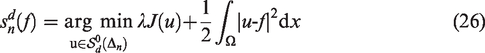
Proposition 3. The total variation functional $J:L^1(\Omega )\to [0,+\infty ]$ satisfies the properties:

(a) J is positively 1-homogeneous, i.e., $J(\mathit{tu})=\mathit{tJ}(u),\forall t\ge 0$ and $\forall u\in \mathit{BV}(\Omega )$ ;

(b) J is convex, i.e., $J(\mathit{tu}+(1-t)v)\le \mathit{tJ}(u)+(1-t)J(v)$ , $\forall t\in [0,1]$ , $\forall u,v\in L^1(\Omega )$ ;

(c) J is lower semicontinuous, i.e., if $(u_n)$ is a sequence which converges in $L^1(\Omega )$ to u, then

$$J(u)\le \underset{n\to \infty }{\lim \inf }J(u_n)$$

(10)

Proof. The proof of the proposition is straightforward with (a) and (b) arising from the definition of the total variation, while (c) is a consequence of Lebesgue Dominated Convergence Theorem.□

To establish the main result of this paper, we need to construct a sequence of smooth functions that converges in $L^1(\Omega )$ for which the equality holds in equation (10). By exploiting the extension property of functions of bounded variation (see Theorem 2 above), we will use the following lemma to achieve this goal.

Lemma 4 ⁴² (Proposition 1.15). Suppose $u\in \mathit{BV}(\Omega )$ . If $A\subset \subset \Omega$ is a relatively compact open subset of Ω such that

$${\displaystyle {\int }_{\partial A}|}Du|=0$$

(11)

then

$${\displaystyle {\int }_A|}Du|=\underset{ϵ\to 0}{\lim }{\displaystyle {\int }_A|}D(u*{\eta }_{ϵ})|$$

(12)

where ${\eta }_{ϵ}(x)={ϵ}^{-2}\eta (x/ϵ)$ and η is radially symmetric mollifier.

Bivariate spline functions

Let Δ be a triangulation of Ω. A spline function on the triangulation Δ is a function s defined on Ω such that for any triangle $T\in \Delta$ , the restriction $s{|}_T$ of s to T is a polynomial. The degree of a spline function is the maximum degree of its restrictions to elements of the triangulation Δ. The space of spline functions of degree d on Δ is denoted by

$${\mathcal{S}}_d^{-1}(\Delta ):=\left\{s:\Omega \to \mathbb{R}:s{|}_T\in {\mathbb{P}}_d\forall T\in \Delta \right\}$$

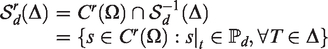
where ${\mathbb{P}}_d$ is the vector space of bivariate polynomials of degree less than or equal to d. The space of smooth spline functions of degree d and order $0\le r\le d,{\mathcal{S}}_d^r(\Delta )$ , is defined by

$$\begin{array}{l}{\mathcal{S}}_d^r(\Delta )=C^r(\Omega )\cap {\mathcal{S}}_d^{-1}(\Delta )\\ =\{s\in C^r(\Omega ):s{|}_t\in {\mathbb{P}}_d,\forall T\in \Delta \}\end{array}$$

Given a basis of the polynomial space ${\mathbb{P}}_d$ , it is easy to see that ${\mathcal{S}}_d^{-1}(\Delta )$ is isomorphic to ${\mathbb{R}}^N$ where $N=\#(\Delta )\left(\begin{array}{c}d+2\\ 2\end{array}\right)$ and $\#(\Delta )$ is the number of triangles in Δ, while the space of smooth splines ${\mathcal{S}}_d^r(\Delta )$ is a subspace of ${\mathbb{R}}^N$ of the form⁴²

$${\mathcal{S}}_d^r(\Delta )\equiv \left\{\mathit{c}\in {\mathbb{R}}^N:A(r)\mathit{c}=\mathbf{0}\right\}$$

(13)

where A(r) is an $(r+1)(d+1)E\times N$ matrix encoding the smoothness condition across the interior edges of the triangulation Δ, and E is the number of interior edges of Δ. Notice that we can use a different basis of ${\mathbb{P}}_d$ for each triangle $T\in \Delta$ and in such instance we shall write

$${\mathcal{S}}_d^{-1}({\Delta }_h)={\displaystyle \prod _{T\in \Delta }{\mathbb{P}}_d^T}$$

For our purposes in this paper, we shall use the Bernstein-Bézier basis of ${\mathbb{P}}_d^T$ for each triangle $T\in \Delta$ .

Spline functions have been used with much success in the numerical computation of partial differential equations using variational methods^44–48 and more recently for the numerical simulation of the Darcy–Stokes equation. ⁴⁹ In general, spline functions may be utilized as approximation spaces to study some classes of variational equations using the Galerkin method. Their appeal to us in this work is twofold. Firstly, bivariate spline functions possess good approximation power in the Sobolev spaces ${\text{W}}^{m,p}(\Omega )$ as illustrated by the following theorem.

Theorem 5 ⁴³ (Theorem 10.2, p. 277). Suppose that Δ is a regular triangulation of Ω of mesh size h > 0. Let $p\in [1,\infty ]$ and $d\in \mathbb{N}$ be given. Then for every $u\in W^{d+1,p}(\Omega )$ , there exists a spline function $s_u\in {\mathcal{S}}_d^0(\Delta )$ such that

$$\left|\right|D_1^{\alpha }{D}_2^{\beta }(u-s_u)|{|}_{L^p(\Omega )}\le K{h}^{d+1-\alpha -\beta }|u{|}_{d+1,p}\forall 0\le \alpha +\beta \le d$$

(14)

where K depends only on d and the smallest angle of Δ, and

$$|u{|}_{d+1,p}={\displaystyle \sum _{\alpha +\beta =d+1}\left|\right|}{D}_1^{\alpha }{D}_2^{\beta }u|{|}_{L^p(\Omega )}$$

Secondly, the differential operators $D_1^{\alpha }{D}_2^{\beta }$ are bounded linear operators between the spaces ${\mathcal{S}}_d^{-1}(\Delta )$ and ${\mathcal{S}}_{d-\alpha -\beta }^{-1}(\Delta )$ . This property is known in the literature as the Markov inequality.

Theorem 6 (Markov inequality,⁴² Theorem 2.32). Let Δ be a triangulation of Ω. Let $p\in [1,\infty )$ and $d\in \mathbb{N}$ be fixed. There exists a constant K depending only on d such that for all nonnegative integers α and β with $0\le \alpha +\beta \le d$ , we have

$$\left|\right|D_1^{\alpha }{D}_2^{\beta }s|{|}_{L^p(\Omega )}\le \frac{K}{{\rho }^{\alpha +\beta }}|\left|s\right|{|}_{L^p(\Omega )},\forall s\in {\mathcal{S}}_d^{-1}(\Delta )$$

(15)

where $\rho =\min \left\{{\rho }_t:t\in \Delta \right\}$ with ρ_t the inradius of the triangle t.

Remark 7. Notice that one can define a spline functions space on any simplicial tiling of the domain Ω and all polynomials based finite element spaces are preferential subspaces of the spline space ${\mathcal{S}}_d^{-1}({\Delta }_h)$ for some choice of d.

Natural images contain structural information in the form of edges and textures. Resolving these entities with continuous spline functions will require fine triangulations which in turn demand high resolution images. An alternative is to use high order spline functions on moderate size triangulations as these are more capable of capturing the variations corresponding to edges than continuous spline functions on such triangulations. The following result gives the relationship between the degree and the order of the spline function to guarantee suitable approximation power in Sobolev spaces.

Theorem 8 ⁴³ (Theorem 10.10). Let $d\ge 3r+2$ and suppose Δ is a regular triangulation of Ω of mesh size h. Then for every $f\in W_q^{d+1}(\Omega )$ , there exists a spline $s\in {\mathcal{S}}_d^r({\Delta }_h)$ such that

$$\left|\right|D_1^{\alpha }{D}_2^{\beta }(u-s_u)|{|}_{L^p(\Omega )}\le K{h}^{d+1-\alpha -\beta }|u{|}_{d+1,p}\forall 0\le \alpha +\beta \le d$$

(16)

If Ω is convex, then the constant K depends only on $r,d$ and the smallest angle on Δ; otherwise K also depends on the Lipschitz constant of the boundary of Ω.

Galerkin approximation with smooth splines

In this section, we describe how we arrive at a family of continuous bivariate spline functions that approximate the minimizer of the functional

$$E_{\lambda }^f(u):=\lambda J(u)+\frac{1}{2}{\displaystyle {\int }_{\Omega }|}u-f{|}^2\text{d}x$$

(17)

Before undertaking the analysis of our approximation method, let us briefly explain why the ROF model is well posed. In fact, Proposition 3 implies that for $f\in L^2(\Omega )$ and $\lambda >0$ fixed, the ROF functional $E_{\lambda }^f$ is strictly convex and lower semi-continuous on $\mathit{BV}(\Omega )\cap L^2(\Omega )$ for the norm of $L^2(\Omega )$ . Therefore, the ROF model (1) has a unique solution and the problem is well posed as illustrated by the following result.

Theorem 9. Let $u_{\lambda }^f\in \mathit{BV}(\Omega )$ be the minimizer of the ROF functional $E_{\lambda }^f(u)$ . Then for any $v\in \mathit{BV}(\Omega )$ , there holds

$$\left||v-u_{\lambda }^f\right|{|}_{L^2}^2\le 2\left(E_{\lambda }^f(v)-E_{\lambda }^f\left(u_{\lambda }^f\right)\right)$$

(18)

and

$$\underset{x\in \Omega }{\inf }f(x)\le u_{\lambda }^f(x)\le \underset{x\in \Omega }{\sup }f(x)\text{ for }\text{a}.\text{e}.\text{x}\in \Omega$$

(19)

Moreover, if $u_{\lambda }^g$ is the minimizer of $E_{\lambda }^g(u)$ , then

$$\left|\right|u_{\lambda }^f-u_{\lambda }^g|{|}_{L^2}\le ||f-g|{|}_{L^2}$$

(20)

Proof. The proof is a simple exercise of convex analysis and uses the characterization of the minimizer of a convex functional using subdifferentials. The complete proof is found in Matamba Messi. ²⁹ □

The approximation of the minimizer of the ROF model by continuous spline functions is possible because the space ${\mathcal{S}}_d^0(\Delta )$ possesses very good approximation power in high-order Sobolev spaces as illustrated by Theorem 5 and a function of bounded variation can be approximated by smooth functions. In using Theorem 5, we will need to control the norm of high order derivatives of the mollification of a BV function. This is done as in the lemma below.

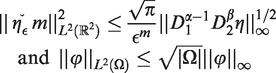
Lemma 10. Let $u\in \mathit{BV}({\mathbb{R}}^2)$ be fixed. Then for any integer $m\ge 0$ , any pair of nonnegative integer $(\alpha ,\beta )$ such that $\alpha +\beta =m+1$ , and any $ϵ>0$ , we have

$$\left||D_1^{\alpha }{D}_2^{\beta }\left({\eta }_{ϵ}*u\right)\right|{|}_{L^1(\Omega )}\le \frac{C}{{ϵ}^m}\left|\mathit{Du}\right|\left({\mathbb{R}}^2\right)$$

(21)

where C is a constant depending only on m and Ω.

Proof. Let $\phi \in C_c^1(\Omega )$ be given. Let α and β be two nonnegative integers such that $\alpha +\beta =m+1$ ; we may assume without loss of generality that $\alpha \ge 1$ . Then, with ${\check{\eta }}_{ϵ}^m(x)=D_1^{\alpha -1}{D}_2^{\beta }{\eta }_{ϵ}(-x)$ we have

$$\begin{array}{l}{\displaystyle {\int }_{\Omega }{D}_1^{\alpha }}{D}_2^{\beta }\left({\eta }_{ϵ}*u\right)\phi \text{d}x=-{\displaystyle {\int }_{{\mathbb{R}}^2}{D}_1^{\alpha -1}}{D}_2^{\beta }({\eta }_{ϵ}*u)\frac{\partial \phi }{\partial x_1}\text{d}x\\ =-{\displaystyle {\int }_{{\mathbb{R}}^2}{D}_1^{\alpha -1}}{D}_2^{\beta }{\eta }_{ϵ}*u\frac{\partial \phi }{\partial x_1}\text{d}x\\ =-{\displaystyle {\int }_{{\mathbb{R}}^2}u}{\check{\eta }}_{ϵ}^m*\frac{\partial \phi }{\partial x_1}\text{d}x\\ =-{\displaystyle {\int }_{{\mathbb{R}}^2}u}\frac{\partial }{\partial x_1}[{\check{\eta }}_{ϵ}^m*\phi ]\text{d}x\end{array}$$

Thus

$${\displaystyle {\int }_{\Omega }{D}_1^{\alpha }}{D}_2^{\beta }({\eta }_{ϵ}*u)\phi \text{d}x\le \left|\right|{\check{\eta }}_{ϵ}^m*\phi \left|{|}_{\infty }\right|\mathit{Du}|({\mathbb{R}}^2)$$

Now by Hölder’s inequality we have

$$\left|\right|{\check{\eta }}_{ϵ}^m*\phi |{|}_{\infty }\le |\left|{\check{\eta }}_{ϵ}^m\right|{|}_{L^2({\mathbb{R}}^2)}\left|\right|\phi |{|}_{L^2(\Omega )}$$

a simple computation shows that

$$\begin{array}{l}\left|\right|{\check{\eta }}_{ϵ}^m|{|}_{L^2({\mathbb{R}}^2)}^2\le \frac{\sqrt{\pi }}{{ϵ}^m}\left||D_1^{\alpha -1}{D}_2^{\beta }\eta \right|{|}_{\infty }^{1/2}\\ \text{and }\left|\right|\phi |{|}_{L^2(\Omega )}\le \sqrt{\left|\Omega \right|}|\left|\phi \right|{|}_{\infty }\end{array}$$

where $\left|\Omega \right|$ is the Lebesgue measure of Ω. Consequently

$${\displaystyle {\int }_{\Omega }{D}_1^{\alpha }}{D}_2^{\beta }\left({\eta }_{ϵ}*u\right)\phi \text{d}x\le \frac{C(m,\eta )}{{ϵ}^m}\left|\right|\phi \left|{|}_{\infty }\right|\mathit{Du}|({\mathbb{R}}^2)$$

(22)

where

$$C(m,\eta )=\sqrt{\pi \left|\Omega \right|}{\max }_{\alpha +\beta =m}\left||D_1^{\alpha }{D}_2^{\beta }\eta \right|{|}_{\infty }^{1/2}$$

(23)

Taking the supremum in equation (22) over all $\phi \in C_c^1(\Omega )$ such that $\left|\right|\phi |{|}_{\infty }\le 1$ , we obtain by duality and a denseness argument that

$$\left||D_1^{\alpha }{D}_2^{\beta }\left({\eta }_{ϵ}*u\right)\right|{|}_{L^1(\Omega )}\le \frac{C\left(m,\eta \right)}{{ϵ}^m}\left|\mathit{Du}\right|({\mathbb{R}}^2)$$

□

Suppose that Ω is endowed with a regular triangulation Δ _h of sise h, and let $d\in \mathbb{N}$ be given. As a finite dimensional space, ${\mathcal{S}}_d^0({\Delta }_h)$ is a closed and convex subset of $L^2(\Omega )$ . Thus, the ROF functional has a unique minimizer in ${\mathcal{S}}_d^0({\Delta }_h)$ . Let $s_h^d(f)$ be the spline function defined by

$$s_h^d(f)=\underset{\text{u}\in {\mathcal{S}}_d^{\text{0}}({\Delta }_h)}{\text{arg} \text{min}}\lambda J(u)\text{+}\frac{\text{1}}{\text{2}}{\displaystyle {\int }_{\Omega }\text{|}}{u-f\text{|}}^{\text{2}}\text{d}x$$

(24)

We are ready to prove that our construction of minimum splines above yields a minimizing sequence for the ROF functional. Let h_n be a monotonically decreasing sequence of real numbers such that $h_n\searrow 0$ as $n\to \infty$ . Let Δ _n be a quasi-regular triangulation of Ω with mesh size h_n and smallest angle θ_n. We have the following result:

Theorem 11. Suppose that the sequence of regular triangulations ${\left\{{\Delta }_n\right\}}_n$ is such that

$$\underset{n\in \mathbb{N}}{\inf }{\theta }_n>\theta >0$$

(25)

Given $d\in \mathbb{N}$ , the sequence ${\{s_n^d(f)\}}_n$ defined by

$$s_n^d(f)=\underset{\text{u}\in {\mathcal{S}}_d^{\text{0}}({\Delta }_n)}{\text{arg} \text{min}}\lambda J(u)\text{+}\frac{\text{1}}{\text{2}}{\displaystyle {\int }_{\Omega }\text{|}}{u-f\text{|}}^{\text{2}}\text{d}x$$

(26)

is minimizing for the ROF functional $E_{\lambda }^f(u)$ .

Proof. Let $T:\mathit{BV}(\Omega )\to \mathit{BV}({\mathbb{R}}^2)$ be the extension operator associated with the $1-$ neighborhood of Ω, the existence of which is guaranteed by Theorem 2. We recall that T is also a bounded linear operator from $W^{1,1}(\Omega )$ into $W^{1,1}({\mathbb{R}}^2)$ , and for any $u\in \mathit{BV}(\Omega )$ , Tu is supported on the the $1-$ neighborhood of Ω.

Let $0<ϵ<1$ and $d\in \mathbb{N}$ be fixed. Let $u_{\lambda }^f$ be the minimizer of $E_{\lambda }^f(u)$ and put $u_{ϵ}^f={\eta }_{ϵ}*T{u}_{\lambda }^f$ . Let $s_{ϵ}^f\in {\mathcal{S}}_d^0({\Delta }_n)$ be as in Theorem 5. Then by Lemma 10, we have

$$\left|\right|u_{ϵ}^f-s_{ϵ}^f|{|}_{W^{1,1}(\Omega )}\le C(d,\theta ){\left(\frac{h_n}{ϵ}\right)}^d$$

(27)

where C depends solely on d and θ. Moreover, since $T:W^{1,1}(\Omega )\to W^{1,1}({\mathbb{R}}^2)$ is bounded, and Tu is compactly supported for every u, it follows from the Poincaré inequality (equation (9)) that

$$\begin{array}{l}\left|\right|u_{ϵ}^f-s_{ϵ}^f|{|}_{L^2(\Omega )}\le ||T(u_{ϵ}^f-s_{ϵ}^f)|{|}_{L^2({\mathbb{R}}^2)}\\ \le C{\displaystyle {\int }_{{\mathbb{R}}^2}|}\nabla (T(u_{ϵ}^f-s_{ϵ}^f))|\text{d}x\\ \le C\left|\right|T(u_{ϵ}^f-s_{ϵ}^f)|{|}_{W^{1,1}({\mathbb{R}}^2)}\\ \le C\left|\right|T\left|{|}_{*}\right||u_{ϵ}^f-s_{ϵ}^f|{|}_{W^{1,1}(\Omega )}\end{array}$$

(28)

with C a universal constant depending only on ${\Omega }_1$ the $1-$ neighborhood of Ω, and $\left|\right|T|{|}_{*}$ is the operator norm of T.

We now show that by choosing a suitable regularization scale ϵ, we achieve the convergence of $E_{\lambda }^f(s_n^d(f))$ to $E_{\lambda }^f(u_{\lambda }^f)$ as $n\to \infty$ . In fact for any $ϵ>0$ , we have

$$\begin{array}{l}{E}_{\lambda }^f\left(s_n^d\left(f\right)\right)-E_{\lambda }^f(u_{\lambda }^f)\\ =︸\underset{\le 0}{E_{\lambda }^f\left(s_n^d\left(f\right)\right)-E_{\lambda }^f(s_{ϵ}^f)}+E_{\lambda }^f(s_{ϵ}^f)-E_{\lambda }^f(u_{ϵ}^f)\\ +E_{\lambda }^f(u_{ϵ}^f)-E_{\lambda }^f(u_{\lambda }^F)\\ \le E_{\lambda }^f(s_{ϵ}^f)-E_{\lambda }^f(u_{ϵ}^f)+E_{\lambda }^f(u_{ϵ}^f)-E_{\lambda }^f(u_{\lambda }^f)\end{array}$$

So to finish the proof, it suffices to show that

$$E_{\lambda }^f(u_{ϵ}^f)\to E_{\lambda }^f(u_{\lambda }^f)$$

and

$$E_{\lambda }^f(s_{ϵ}^f)\to E_{\lambda }^f(u_{ϵ}^f)$$

as $n\to \infty$ for a suitable choice of ϵ. First, we observe that the convergence of $E_{\lambda }^f(u_{ϵ}^f)$ to $E_{\lambda }^f(u_{\lambda }^f)$ follows from the fact that

$$u_{ϵ}^f\underset{ϵ\to 0}{\overset{L^2(\Omega )}{\to }}{u}_{\lambda }^f$$

and by Lemma 4 applied to

$$T{u}_{\lambda }^f:\left|D{u}_{ϵ}^f\right|(\Omega )\underrightarrow{\stackrel{ϵ\to 0}{\hspace{0.17em}}}\left|\mathit{DT}{u}_{\lambda }^f\right|(\overline{\Omega })=J(u)$$

Second, by the triangle inequality and direct calculation we have

$$\begin{array}{l}\left|E_{\lambda }^f(s_{ϵ}^f)-E_{\lambda }^f(u_{ϵ}^f)\right|\\ \le \lambda {\displaystyle {\int }_{\Omega }|}\nabla (s_{ϵ}^f-u_{ϵ}^f)|\mathit{dx}+\frac{1}{2}[\left|\right|s_{ϵ}^f-u_{ϵ}^f|{|}_{L^2(\Omega )}^2\\ +2\left|\right|u_{ϵ}^f-f\left|{|}_{L^2(\Omega )}\right||u_{ϵ}^f-s_{ϵ}^f|{|}_{L^2(\Omega )}]\end{array}$$

We continue to rearrange the second term to have

$$\begin{array}{l}\left|E_{\lambda }^f(s_{ϵ}^f)-E_{\lambda }^f(u_{ϵ}^f)\right|\\ \le \lambda {\displaystyle {\int }_{\Omega }\left|\nabla (s_{ϵ}^f-u_{ϵ}^f)\right|}\text{d}x+\frac{1}{2}\left|\right|s_{ϵ}^f-u_{ϵ}^f|{|}_{L^2(\Omega )}\\ ·(||u_{ϵ}^f-s_{ϵ}^f|{|}_{L^2(\Omega )}+2\left|\right|u_{ϵ}^f-f|{|}_{L^2(\Omega )})\\ \le \left[\lambda +\frac{1}{2}\left|\right|u_{ϵ}^f-s_{ϵ}^f|{|}_{L^2(\Omega )}+||u_{ϵ}^f-f|{|}_{L^2(\Omega )}\right]\end{array}\begin{array}{l}·\left[\left|\right|u_{ϵ}^f-s_{ϵ}^f|{|}_{W^{1,1}(\Omega )}+||u_{ϵ}^f-s_{ϵ}^f|{|}_{L^2(\Omega )}\right]\\ \le (1+C|\left|T\right|{|}_{*})[\lambda +\frac{C\left|\right|T|{|}_{*}}{2}\left|\right|u_{ϵ}^f-s_{ϵ}^f|{|}_{W^{1,1}(\Omega )}\\ +\left|\right|u_{ϵ}^f-f|{|}_{L^2}]\left|\right|u_{ϵ}^f-s_{ϵ}^f|{|}_{W^{1,1}(\Omega )}\end{array}$$

where we have used the estimate (equation (28)).

Now, using the estimate (equation (27)) and letting $ϵ=h_n^{1/4d}$ , we infer from the latter inequality that

$$\begin{array}{l}|E_{\lambda }^f(s_{ϵ}^f)-E_{\lambda }^f(u_{ϵ}^f)|\le (1+C|\left|T\right|{|}_{*})C(d,\theta )\\ \times [\lambda +C(d,\theta ,T)h_n^{d-1/4}+C(f,u_{\lambda }^f)]h_n^{d-1/4}\end{array}$$

where

$$C(f,u_{\lambda }^f)=\left|\right|f\left|{|}_{L^2(\Omega )}\underset{0<ϵ<1}{\sup }\right|\left|u_{ϵ}^f\right|{|}_{L^2(\Omega )}$$

$$C\left(d,\theta ,T\right):=\frac{C\left|\right|T|{|}_{*}C(d,\theta )}{2}$$

Thus, $E_{\lambda }^f(s_n(f))\to E_{\lambda }^f(u_{\lambda }^f)$ as $h_n\to 0$ and the proof is complete.□

Remark 12. It is easy to construct a sequence of triangulation with vanishing mesh sizes for which condition (25) is satisfied. Starting from a triangulation ${\Delta }_0$ of Ω with smallest angle θ₀ and mesh size h₀, a sequence of triangulations Δ _n is generated via successive refinements as follows: Given Δ _n , we obtain ${\Delta }_{n+1}$ by subdividing each triangle $t\in {\Delta }_n$ into four triangles by connecting the midpoints of the edges of t. The resulting triangulation ${\Delta }_{n+1}$ has mesh size $h_0{2}^{-n-1}$ and smallest angle θ₀.

Corollary 13. Under the assumptions of Theorem 11, the sequence ${\{s_n^d(f)\}}_n$ satisfies the following two properties:

$$s_n^d(f)\stackrel{L^p(\Omega )}{\to }{u}_{\lambda }^f\text{ as }n\to \infty ,\hspace{1em}\text{for any }p\in [1,2]$$

(29)

and

$$J(s_n^d(f))\to J(u)\hspace{1em}\text{ as }n\to \infty$$

(30)

Proof. Since Ω is a bounded domain it suffices to establish (29) for p = 2. The result for $1\le p<2$ follows from the fact that $L^2(\Omega )$ is canonically embedded into $L^p(\Omega )$ . The case p = 2 follows easily from Theorem 9 and Theorem 11. Indeed, owing to equation (18), we have for all $n\in \mathbb{N}$

$$\left|\right|s_n^d(f)-u_{\lambda }^f|{|}_{L^2(\Omega )}^2\le 2\left(E_{\lambda }^f(s_n^d(f))-E_{\lambda }^f(u_{\lambda }^f)\right)$$

thus by Theorem 11 above, we have

$$\left|\right|s_n^d(f)-u_{\lambda }^f|{|}_{L^2(\Omega )}^2\to 0$$

as $n\to \infty$ . Finally, since

$$\begin{array}{l}J(s_n^d(f))-J(u)\\ =\frac{1}{\lambda }[E_{\lambda }^f(s_n^d(f))-E_{\lambda }^f(u_{\lambda }^f)+\frac{1}{2}||u_{\lambda }^f-f|{|}_{L^2}^2\\ -\frac{1}{2}\left|\right|s_n^d(f)-f|{|}_{L^2}^2]\le \frac{1}{\lambda }[E_{\lambda }^f(s_n^d(f))-E_{\lambda }^f(u_{\lambda }^f)\\ +\frac{1}{2}\left|\right|u_{\lambda }^f-s_n^d(f)\left|{|}_2\right||u_{\lambda }^f+s_n^d(f)-2f|{|}_2]\\ \le \frac{1}{\lambda }{(E_{\lambda }^f(s_n^d(f))-E_{\lambda }^f(u_{\lambda }^f))}^{1/2}\\ ·\left[E_{\lambda }^f(s_n^d(f))-E_{\lambda }^f(u_{\lambda }^f)+\left|\right|u_{\lambda }^f+s_n^d(f)-2f|{|}_2\right]\end{array}$$

and the sequence ${\left\{\right||s_n^d(f)|{|}_2\}}_n$ is bounded, thanks to Theorem 11 taking the limit of the latter identity as $n\to \infty$ yields (30) and the proof is complete.□

Remark 14. Bartels [5] establish Corollary 13 for the case d = 1. Our result generalizes and is applicable to higher order finite elements under h-refinement for which property (equation (14)) holds with infinitely differentiable functions.

Remark 15. The results of Theorem 20 and Corollary 13 hold if we replace ${\mathcal{S}}_d^0({\Delta }_h)$ with ${\mathcal{S}}_d^r({\Delta }_h)$ in the definition of the spline minimizer $s_h^d(f)$ provided that the hypotheses of Theorem 8 hold. In particular, we must have $d\ge 3r+2$ and a family of regular triangulations.

Fixed point relaxation algorithm

The challenge in computing with the ROF model stems from the fact that the objective functional $E_{\lambda }^f$ is not Gâteaux differentiable; so the solution cannot be described in terms of the first variation of $E_{\lambda }^f$ . The reason why we cannot use the standard machinery of calculus of variation to solve equation (24) is that the associated Lagrangian

$$L\left(\mathit{p},z,x\right)=\lambda \left|\mathit{p}\right|+\frac{1}{2}{\left(z-f\right)}^2,\forall \left(\mathit{p},z,x\right)\in {\mathbb{R}}^2\times \mathbb{R}\times {\mathbb{R}}^2$$

is not differentiable with respect to $\mathit{p}$ at the origin $\mathit{p}=\mathbf{0}$ . One way to mitigate this difficulty is to find a differentiable relaxation of the Lagrangian L such that the corresponding energy functional is a perturbation of $E_{\lambda }^f(u)$ ; that approach has been successfully used on at least three occasions in the literature.^8,9,27

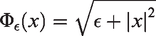
Following Chambolle and Lions,⁹ we let ${\Phi }_{ϵ}$ be the real-valued function defined on ${\mathbb{R}}^2$ by

$${\Phi }_{ϵ}(x)=\{\begin{array}{ll}\frac{|x{|}^2}{2ϵ}+\frac{ϵ}{2}\hfill & \text{ if }\left|x\right|\le ϵ\hfill \\ \left|x\right|\hfill & \text{ if }\left|x\right|>ϵ\hfill \end{array}$$

(31)

and consider the optimization problem

$$\underset{u\in {\mathcal{S}}_d^{\text{0}}({\Delta }_h)}{\text{arg} \text{min}}\left\{E_{\lambda ,ϵ}^f(u):\text{=}\lambda {\displaystyle {\int }_{\Omega }{\Phi }_{ϵ}}(\nabla u)\text{d}x+\frac{\text{1}}{\text{2}}{\displaystyle {\int }_{\Omega }\text{|}}{u-f\text{|}}^{\text{2}}\text{d}x\right\}$$

(32)

It is easy to check that the functional $E_{\lambda ,ϵ}^f$ is strictly convex and lower semicontinuous on ${\mathcal{S}}_d^0({\Delta }_h)$ with respect to the L²-norm. Consequently, the minimization problem (equation (32)) has a unique solution that we denote $s_h^d(f,ϵ)$ . We now show that the family of functional $E_{\lambda ,ϵ}^f$ converges uniformly to $E_{\lambda }^f$ and the minimizers $s_h^d(f,ϵ)$ converge to $s_h^d(f)$ as ϵ goes to zero.

Proposition 16. The family of functionals $E_{\lambda ,ϵ}^f(u)$ converges uniformly in ${\mathcal{S}}_d^0({\Delta }_h)$ to $E_{\lambda }^f(u)$ and $s_h^d(f,ϵ)\stackrel{L^2(\Omega )}{\to }{s}_h^d(f)$ as $ϵ\searrow 0$ . Furthermore, under the assumptions of Theorem 11, we have $s_h^d(f,h^{1/4d})\stackrel{L^2(\Omega )}{\to }{u}_{\lambda }^f$ as h goes to 0.

Proof. Let $\Phi$ be the continuous function defined on ${\mathbb{R}}^2$ by $\Phi (x)=\left|x\right|=\sqrt{x_1^2+x_2^2}$ . It is easy to show that

$$\underset{x\in {\mathbb{R}}^2}{\sup }|{\Phi }_{ϵ}(x)-\Phi (x)|\le ϵ$$

Therefore, for any $u\in {\mathcal{S}}_d^0({\Delta }_h)$ we have the estimate

$$|E_{\lambda ,ϵ}^f(u)-E_{\lambda }^f(u)|\le \lambda {\displaystyle {\int }_{\Omega }\left|{\Phi }_{ϵ}(\nabla u)-\Phi (\nabla u)\right|}\text{d}x\le \lambda \left|\Omega \right|ϵ$$

and it follows that $E_{\lambda ,ϵ}^f$ converges uniformly in ${\mathcal{S}}_d^0({\Delta }_h)$ to $E_{\lambda }^f$ .

Next, we note that Theorem 9 remains true on ${\mathcal{S}}_d^0({\Delta }_h)$ . Therefore, rewriting equation (18) in ${\mathcal{S}}_d^0({\Delta }_h)$ for $s_h^d(f)$ , we obtain

$$\begin{array}{l}\left|\right|s_h^d(f,ϵ)-s_h^d(f)|{|}_{L^2(\Omega )}^2\\ \le 2(E_{\lambda }^f(s_h^d(f,ϵ))-E_{\lambda }^f(s_h^d(f)))\\ \le 2(E_{\lambda }^f(s_h^d(f,ϵ))-E_{\lambda ,ϵ}^f(s_h^d(f,ϵ)))\\ +\text{}2(E_{\lambda ,ϵ}^f(s_h^d(f,ϵ))-E_{\lambda }^f(s_h^d(f)))\\ \le 2(\lambda |\Omega |ϵ+︸\underset{\le 0}{E_{\lambda ,ϵ}^f(s_h^d(f,ϵ))-E_{\lambda ,ϵ}^f(s_h^d(f))}\\ +E_{\lambda ,ϵ}^f(s_h^d(f))-E_{\lambda }^f(s_h^d(f)))\\ \le 4\lambda ϵ\left|\Omega \right|\end{array}$$

Thus, $\left|\right|s_h^d(f,ϵ)-s_h^d(f)|{|}_{L^2(\Omega )}\le 2\sqrt{\lambda \left|\Omega \right|ϵ},$ and it follows that $s_h^d(f,ϵ)$ converges to $s_h^d(f)$ in $L^2(\Omega )$ as ϵ goes to 0. Finally, by the triangle inequality we have

$$\begin{array}{c}\left|\right|s_h^d(f,h^{1/4d})-u_{\lambda }^f|{|}_{L^2(\Omega )}\le 2\sqrt{\lambda \left|\Omega \right|h^{1/4d}}+||s_h^d(f)-u_{\lambda }^f|{|}_{L^2(\Omega )}\end{array}$$

$$ Taking the limit of the latter inequality as h goes to 0 and using Corollary 3.5, it follows that $s_h^d(f,h^{1/4d})$ converges to $u_{\lambda }^f$ in $L^2(\Omega )$ as h goes to 0.□

Unlike the spline ROF model (24) for which we cannot use the first variation to characterize the solution, the functional $E_{\lambda ,ϵ}^f$ associated with the relaxation problem (equation (32)) is Gâteaux differentiable. Therefore, the spline function $s_{h,ϵ}^d(f)$ is characterized by:

Proposition 17. A function $u\in {\mathcal{S}}_d^0({\Delta }_h)$ is the minimizer of the functional $E_{\lambda ,ϵ}^f$ in ${\mathcal{S}}_d^0({\Delta }_h)$ if and only if u satisfies the variational equation

$$\lambda {\displaystyle {\int }_{\Omega }\frac{1}{ϵ\vee |\nabla u|}}\nabla u·\nabla s\text{d}x+{\displaystyle {\int }_{\Omega }(u-f)}s\text{d}x=0$$

(33)

for all $s\in {\mathcal{S}}_d^0({\Delta }_h)$ , where $a\vee b:=\max (a,b)$ .

Proof. First, we observe that $E_{\lambda ,ϵ}^f(u)$ is Gâteaux differentiable with directional derivatives at any point $u\in {\mathcal{S}}_d^0({\Delta }_h)$ given by

$$〈d{E}_{\lambda ,ϵ}^f(u),s〉=\lambda {\displaystyle {\int }_{\Omega }\frac{1}{ϵ\vee |\nabla u|}}\nabla u·\nabla s\text{d}x+{\displaystyle {\int }_{\Omega }(u-f)}s\text{d}x$$

$$\forall s\in {\mathcal{S}}_d^0({\Delta }_h)$$

(34)

Therefore, u is a minimizer of $E_{\lambda ,ϵ}^f(u)$ in ${\mathcal{S}}_d^0({\Delta }_h)$ if and only if $d{E}_{\lambda ,ϵ}^f(u)=0$ , i.e. (equation (33)) holds.□

We now set up the variational equation (33) as a fixed point equation for a nonlinear operator on ${\mathcal{S}}_d^0({\Delta }_h)$ . Fix $u\in {\mathcal{S}}_d^0({\Delta }_h)$ and define the bilinear form $L[u,\lambda ]$ on ${\mathcal{S}}_d^0({\Delta }_h)$ by

$$L[u,\lambda ](v,w):=\lambda {\displaystyle {\int }_{\Omega }\frac{1}{ϵ\vee |\nabla u|}}\nabla v·\nabla w\text{d}x+{\displaystyle {\int }_{\Omega }v}w\text{d}x$$

By Markov Inequality (Theorem 6) $L[u,\lambda ]$ is a continuous, coercive bilinear form on the Hilbert space ${\mathcal{S}}_d^0({\Delta }_h)$ as a subspace of $L^2(\Omega )$ . Thus, by Lax–Milgram Theorem ⁵⁰ (Theorem 2.7.7), for any $f\in L^2(\Omega )$ the equation

$$L[u,\lambda ](v,w)={\displaystyle {\int }_{\Omega }f}w\mathit{dx}\forall w\in {\mathcal{S}}_d^0({\Delta }_h)$$

has a unique solution in ${\mathcal{S}}_d^0({\Delta }_h)$ that we denote by $L[u,\lambda ]f$ . Moreover, since $L[u,\lambda ]$ is symmetric $L[u,\lambda ]f$ is characterized by

$$L[u,\lambda ]f=\underset{\text{v}\in {\mathcal{S}}_d^{\text{0}}({\Delta }_h)}{\text{arg} \text{min}}\lambda {\displaystyle {\int }_{\Omega }\frac{\text{|}\nabla {v\text{|}}^{\text{2}}\text{d}x}{ϵ\vee \text{|}\nabla u\text{|}}}\text{+}{\displaystyle {\int }_{\Omega }\text{|}}{v-f\text{|}}^{\text{2}}\text{d}x$$

(35)

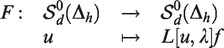
Hence for $f\in L^2(\Omega )$ fixed, we define the nonlinear operator

$$\begin{array}{llll}F:& {\mathcal{S}}_d^0({\Delta }_h)& \to & {\mathcal{S}}_d^0({\Delta }_h)\\ & u& \mapsto & L[u,\lambda ]f\end{array}$$

It is easily shown using the characterizing equation (35) for $L[u,\lambda ]f$ and the dominated convergence theorem that the operator F is continuous. Furthermore, Proposition 17 above defines $s_{h,ϵ}^d(f)$ as a fixed point of F. So we may compute $s_{h,ϵ}^d(f)$ using the fixed point iterative scheme presented and analyzed below.

Algorithm 18. Start from any bounded nonnegative function $v^0\in {\mathcal{S}}_d^0({\Delta }_h)$ and for $n\ge 0$ , let

$$u_{n+1}=\underset{u\in {\text{S}}_d^{\text{0}}({\Delta }_{\text{h}})}{\text{arg} \text{min}}\lambda {\displaystyle {\int }_{\Omega }{v}_n}\text{|}\nabla {u\text{|}}^{\text{2}}\mathrm{d}x\text{+}{\displaystyle {\int }_{\Omega }\text{|}}{u-f\text{|}}^{\text{2}}\text{d}x$$

(36a)

$$v_{n+1}:=\underset{\text{0}<v\le \text{1/}ϵ}{\text{arg} \text{min}}{\displaystyle {\int }_{\Omega }v}\text{|}\nabla u_{n\text{+1}}{\text{|}}^{\text{2}}\text{+}\frac{\text{1}}{v}\mathrm{d}x\text{=}\frac{\text{1}}{ϵ\vee \text{|}\nabla u_{n\text{+1}}\text{|}}$$

(36b)

A standard argument using Lax-Milgram Theorem (see Brezis,39 Corollary 5.8 p. 140) shows that $u_{n+1}$ is characterized by the variational equation

$$\lambda {\displaystyle {\int }_{\Omega }{v}_n}\nabla u_{n+1}·\nabla s\text{d}x+{\displaystyle {\int }_{\Omega }(u_{n+1}-f)}s\text{d}x=0$$

(37)

for all $s\in {\mathcal{S}}_d^0({\Delta }_h)$ . The existence and uniqueness of $u_{n+1}$ follows by observing that the bilinear form

$$L[u_n](u,v):={\displaystyle {\int }_{\Omega }\lambda }{v}_n\nabla u·\nabla v+\mathit{uv}\text{d}x$$

is continuous—thanks to Theorem 6—and coercive on ${\mathcal{S}}_d^0({\Delta }_h)\times {\mathcal{S}}_d^0({\Delta }_h)$ with respect to the L²-norm. Consequently, the equation (37) has a unique solution.

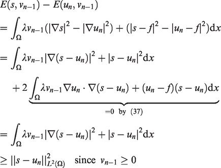
We fix $ϵ>0$ and for the sake of notation conciseness, consider the functional E defined by

$$E(u,v)={\displaystyle {\int }_{\Omega }\lambda }\left(v\right|\nabla u{|}^2+\frac{1}{v})\text{d}x+{\displaystyle {\int }_{\Omega }|}u-f{|}^2\text{d}x$$

(38)

It is easy to check that

$$u_{n+1}=\underset{u\in {\mathcal{S}}_d^{\text{0}}({\Delta }_h)}{\text{arg} \text{min}}E(u,v_n)$$

(39a)

$$v_{n+1}=\underset{\text{0}<v\le \text{1/}ϵ}{\text{arg} \text{min}}E(u_{n\text{+1}},v)$$

(39b)

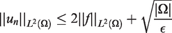
Lemma 19. The sequence ${\left\{u_n\right\}}_n$ is bounded in $H^1(\Omega )$ and satisfies for all $n\in \mathbb{N}$ , and any $s\in {\mathcal{S}}_d^0({\Delta }_h)$

$$\left|\right|s-u_n|{|}_{L^2(\Omega )}^2\le E(s,v_{n-1})-E(u_n,v_{n-1})$$

(40)

In particular, we have for all $n\in \mathbb{N}$

$$\left|\right|u_{n+1}-u_n|{|}_{L^2(\Omega )}^2\le E(u_n,v_n)-E(u_{n+1},v_{n+1})$$

(41)

Proof. We observe that in view of Theorem 6, proving the boundedness of $\left\{u_n\right\}$ in $H^1(\Omega )$ is equivalent to proving its boundedness in $L^2(\Omega )$ . Let $n\in \mathbb{N}$ be given. Then by definition of u_n, we have

$$\begin{array}{l}E(u_n,v_{n-1})\le E(0,v_{n-1})\\ =\left|\right|f|{|}_{L^2}^2+{\displaystyle {\int }_{\Omega }\frac{1}{v_{n-1}}}\text{d}x\le |\left|f\right|{|}_{L^2}^2+\frac{\left|\Omega \right|}{ϵ}\end{array}$$

Consequently, we get $\left|\right|u_n-f|{|}_{L^2(\Omega )}^2\le |\left|f\right|{|}_{L^2(\Omega )}^2+\frac{\left|\Omega \right|}{ϵ}$ , and deduce by the triangle inequality that

$$\left|\right|u_n|{|}_{L^2(\Omega )}\le 2|\left|f\right|{|}_{L^2(\Omega )}+\sqrt{\frac{\left|\Omega \right|}{ϵ}}$$

We now show that $\left|\right|u_n-s|{|}_{L^2(\Omega )}^2\le E(s,v_{n-1})-E(u_n,v_{n-1}).$ For any $s\in {\mathcal{S}}_d^0({\Delta }_h)$ , we have

$$\begin{array}{l}E(s,v_{n-1})-E(u_n,v_{n-1})\\ ={\displaystyle {\int }_{\Omega }\lambda }{v}_{n-1}(|\nabla s{|}^2-|\nabla u_n{|}^2)+(|s-f{|}^2-|u_n-f{|}^2)\text{d}x\\ ={\displaystyle {\int }_{\Omega }\lambda }{v}_{n-1}|\nabla (s-u_n){|}^2+|s-u_n{|}^2\mathrm{d}x\\ +2︸\underset{=0\text{ by }(37)}{{\displaystyle {\int }_{\Omega }\lambda }{v}_{n-1}\nabla u_n·\nabla (s-u_n)+(u_n-f)(s-u_n)\text{d}x}\\ ={\displaystyle {\int }_{\Omega }\lambda }{v}_{n-1}|\nabla (s-u_n){|}^2+|s-u_n{|}^2\text{d}x\\ \ge \left|\right|s-u_n|{|}_{L^2(\Omega )}^2\text{ since }{v}_{n-1}\ge 0\end{array}$$

In particular for any $n\in \mathbb{N}$ ,

$$\begin{array}{l}\left|\right|u_{n+1}-u_n|{|}_{L^2(\Omega )}^2\le E(u_n,v_n)-E(u_{n+1},v_n)\\ =E(u_n,v_n)-E(u_{n+1},v_{n+1})\\ +︸\underset{\le 0\text{ by }(39)}{E(u_{n+1},v_{n+1})-E(u_{n+1},v_n)}\\ \le E(u_n,v_n)-E(u_{n+1},v_{n+1})\end{array}$$

Thus, the sequence ${\{E(u_n,v_n)\}}_n$ is monotone nonincreasing and $\left|\right|u_n-u_{n+1}|{|}_{L^2(\Omega )}\to 0$ .□

Theorem 20. The sequence ${\left\{u_n\right\}}_n$ constructed in Algorithm 4.3 converges in $L^2(\Omega )$ to the minimizer $s_h^d(f,ϵ)$ of $E_{\lambda ,ϵ}^f(u)$ .

Proof. In view of Proposition 17, it suffices to show that any cluster point u of the sequence ${\left\{u_n\right\}}_n$ with respect to the L²-norm satisfies the Euler-Lagrange equation (33). To begin, we note that the sequence ${\left\{u_n\right\}}_n$ has at least one cluster point as a bounded sequence in a finite dimensional normed vector space.

Let u be any cluster point of ${\left\{u_n\right\}}_n$ in $L^2(\Omega )$ and ${\left\{u_{n_k}\right\}}_k$ a subsequence such that $u_{n_k}\stackrel{L^2(\Omega )}{\to }u$ . Since

$$\left|\right|u_{n_k+1}-u_{n_k}|{|}_{L^2(\Omega )}\to 0$$

it follows that $u_{n_k+1}\stackrel{L^2(\Omega )}{\to }u$ as well. By Markov inequality—Theorem 6—we also have

$$u_{n_k}\underset{k\to \infty }{\overset{H^1(\Omega )}{\to }}u,\text{ and }{u}_{n_k+1}\underset{k\to \infty }{\overset{H^1(\Omega )}{\to }}u$$

Therefore, by Lebesgue dominated convergence theorem, we get

$$v_{n_k}=\frac{1}{|\nabla u_{n_k}|}\wedge \frac{1}{ϵ}\underset{k\to \infty }{\overset{L^2(\Omega )}{\to }}\frac{1}{|\nabla u|}\wedge \frac{1}{ϵ}=\frac{1}{ϵ\vee |\nabla u|}$$

Next, we establish that u satisfies the variational equation

$$\lambda {\displaystyle {\int }_{\Omega }\frac{1}{ϵ\vee |\nabla u|}}\nabla u·\nabla s\text{d}x+{\displaystyle {\int }_{\Omega }(u-f)}s\text{d}x=0$$

(42)

for all $s\in {\mathcal{S}}_d^0({\Delta }_h)$ . Indeed by definition of $u_{n_k+1}$ , there holds

$$\lambda {\displaystyle {\int }_{\Omega }{v}_{n_k}}\nabla s·\nabla u_{n_k+1}\text{d}x+{\displaystyle {\int }_{\Omega }(u_{n_k+1}-f)}s\text{d}x=0$$

(43)

for all $k\in \mathbb{N}$ . Since $\nabla u_{n_k+1}$ converges strongly to $\nabla u$ in $L^2(\Omega )\times L^2(\Omega )$ and $v_{n_k}\nabla s$ converges strongly to $\nabla s/(ϵ\vee |\nabla u|)$ , it follows that

$${\displaystyle {\int }_{\Omega }{v}_{n_k}}\nabla s·\nabla u_{n_k+1}\text{d}x\to {\displaystyle {\int }_{\Omega }\frac{1}{ϵ\vee |\nabla u|}}\nabla u·\nabla s\text{d}x$$

(44)

as $k\to \infty$ . Similarly, as $u_{n_k+1}$ converges strongly to u in $L^2(\Omega )$ , we infer that

$${\displaystyle {\int }_{\Omega }(u_{n_k+1}-f)}s\text{d}x\to {\displaystyle {\int }_{\Omega }(u-f)}s\text{d}x\text{\hspace{1em}as }k\to \infty$$

(45)

On passing to the limit as $k\to \infty$ in (43) and taking into account equations (44) and (45), we obtain equation (42) and the proof is complete.□

Remark 21. Many choices of the function ${\Phi }_{ϵ}\in C^1({\mathbb{R}}^2)$ for constructing a relaxation of the ROF functional are possible; presumably any choice of a family of convex continuously differentiable functions that yields a uniform approximation of the Euclidian norm should do the trick. A common choice seen in the literature and introduced by Acar and Vogel⁸ is the function

$${\Phi }_{ϵ}(x)=\sqrt{ϵ+|x{|}^2}$$

Remark 22. For d = 1 the relaxation algorithm is not necessary as a direct algorithm for computing the minimizers is readily available. Indeed, in this case the objective functional reads

$$\begin{array}{c}{E}_{\lambda }^f(s)=\underset{\begin{array}{c}q\in {\mathcal{S}}_0^{-1}({\Delta }_h)\times {\mathcal{S}}_0^{-1}({\Delta }_h)\\ |q{|}_T{|}_2\le 1, T\in {\Delta }_h\end{array}}{\sup }\{\lambda {\displaystyle {\int }_{\Omega }\nabla }s·q\text{d}x+\frac{1}{2}{\displaystyle {\int }_{\Omega }|}s-f{|}^2\text{d}x\}\end{array}$$

(46)

and the ROF model over the continuous affine functions turns into the saddle-point problem

$$\begin{array}{l}{u}_{\lambda }^f=\text{arg} {\text{min}}_{\text{s}\in {\mathcal{S}}_{\text{1}}^{\text{0}}({\Delta }_{\text{h}})}\underset{\begin{array}{l}\text{q}\in {\mathcal{S}}_{\text{0}}^{\text{-1}}({\Delta }_{\text{h}})\times {\mathcal{S}}_{\text{0}}^{\text{-1}}({\Delta }_{\text{h}})\\ |q_T{|}_2\le 1, T\in {\Delta }_h\end{array}}{\sup }\{\lambda {\displaystyle {\int }_{\Omega }\nabla }s·q\text{d}x\\ +\frac{1}{2}{\displaystyle {\int }_{\Omega }|}s-f{|}^2\text{d}x\}\end{array}$$

(47)

One can then solve the latter problem using the first-order primal dual algorithm studied by Chambolle and Pock.⁵⁰ Indeed, Bartels ⁵² has studied it in details and provided ample evidence of convergence.

Applications to digital image processing

In this section, we report the results of some numerical experiments done using the algorithm described above on digital images. It is well known (some of these observations have been confirmed by theory) that:

the ROF model is excellent on piecewise constant images up to a reduction in contrast;

finite difference algorithms for the ROF model are vulnerable to the staircase effect, whereby smooth regions are recovered as mosaics of piecewise constant subregions;

total variation based image enhancement methods are ineffective in discriminating textures from noise at well mixed scales.

Two examples illustrating the issues raised above are provided, using both the finite difference and spline methods. However, we will see that the staircase effect is tamed by the spline method.

A digital total variation spline model

A digital image is a quantization of a light intensity field. For our purposes here, we model digital images as samples or quantization of functions defined on a domain Ω. For example, an image with resolution M × N could be thought of as the evaluation on the grid $\{(i,j):1\le i\le M, 1\le j\le N\}$ of a function f defined on $\Omega =(1/2, M+1/2)\times (1/2, N+1/2)$ ; alternatively we could think of it as a sample of local averages of the function f on squares centered at (i, j).

The algorithm described in the previous section assumes that f is a function on the continuum domain Ω, however, digital images are merely samples of such functions. Therefore for processing digital images with the ROF model on spline spaces, we should try to estimate the function f from its samples $\{f_i:1\le i\le P\}$ . One way to do these is to use any of the penalized spline fitting method introduced by Awanou et al.⁵² The problem with this approach is that the preliminary estimation step significantly modifies the input data. When the estimated function is fed to the ROF model, we cannot easily discriminate the contribution of the total variation smoothing procedure on the final output.

In order to clearly illustrate the effect of the total variation smoothing procedure in digital image processing, we solve the following variant of the spline minimization problem (equation (24))

$$\underset{s\in {\mathcal{S}}_d^r({\Delta }_h)}{\text{arg} \text{min}}\lambda {\displaystyle {\int }_{\Omega }\text{|}}\nabla s|\mathrm{d}x\text{+}\frac{\text{1}}{\text{2}}{\displaystyle \sum _{T\in {\Delta }_h}{\displaystyle \sum _{x_i\in T}|}}s(x_i){-f}_i{|}^{\text{2}}$$

(48)

where P is the total number of pixels and $s(x_i)$ is the value of the spline function s at the pixel location $x_i\in \Omega$ . We have simply replaced the continuum L² fidelity term with a discrete counterpart based on the available data. In general, the optimization problem (50) may not have a solution unless the pixel locations $\mathcal{D}=\{x_i\in \Omega :1\le i\le P\}$ are well distributed across the triangles of Δ _h .

Theorem 23. Suppose that the pixel locations

$$\mathcal{D}=\{x_i\in \Omega :1\le i\le P\}$$

are such that, the mapping

$$N_D(s)={\left({\displaystyle \sum _{T\in {\Delta }_h}{\displaystyle \sum _{x_i\in T}s}}{(x_i)}^2\right)}^{1/2}$$

(49)

is a norm on ${\mathcal{S}}_d^r({\Delta }_h)$ . Then there exists a unique spline function $s_h\in {\mathcal{S}}_d^r({\Delta }_h)$ such that

$$s_h=\underset{\text{s}\in {\mathcal{S}}_{\text{d}}^{\text{r}}({\Delta }_{\text{h}})}{\text{arg} \text{min}}{\text{E}}_{\text{d}}(\text{s})$$

where

$$E_d(s):=\lambda {\displaystyle {\int }_{\Omega }|}\nabla s|\text{d}x+\frac{1}{2}{\displaystyle \sum _{T\in {\Delta }_h}{\displaystyle \sum _{x_i\in T}|}}s(x_i)-f_i{|}^2$$

Proof. Notice that $E_d(s)$ is strictly convex and continuous on ${\mathcal{S}}_d^r({\Delta }_h)$ ; therefore $E_d(s)$ has at most one minimizer in ${\mathcal{S}}_d^r({\Delta }_h)$ . Let ${\left\{s_n\right\}}_n$ be a minimizing sequence of E_d, i.e $E_d(s_n)$ converges to $\underset{s\in {\mathcal{S}}_d^r({\Delta }_h)}{\inf }{E}_d(s)$ . The sequence ${\left\{N_D(s_n)\right\}}_n$ is bounded, and since we assume that N_D is a norm and ${\mathcal{S}}_d^r({\Delta }_h)$ is finite dimensional, it follows that any subsequence of ${\left\{s_n\right\}}_n$ has a convergent subsequence with respect to the norm N_D. Now, if $s^{*}$ is the limit of a subsequence of ${\left\{s_n\right\}}_n$ , then by continuity of E_d we have $E_d(s^{*})=\underset{s\in {\mathcal{S}}_d^r({\Delta }_h)}{\inf }{E}_d(s)$ and $s^{*}$ is a minimizer of E_d. Thus, the set of minimizers of E_d is nonempty. Finally, since E_d is strictly convex and limit points of ${\left\{s_n\right\}}_n$ are minimizers of E_d, we infer that the minimizing sequence ${\left\{s_n\right\}}_n$ converges to the unique minimizer s_h of E_d.□

Remark 24. The condition (49) is equivalent to saying that the pixel locations set D is determining for the space of piecewise polynomials ${\mathcal{S}}_d^{-1}({\Delta }_h)$ , that is every element $s\in {\mathcal{S}}_d^{-1}({\Delta }_h)$ is uniquely determined by the values of $s{|}_T$ at the pixel locations ${\mathcal{D}}_T=\mathcal{D}\cap T$ for every $T\in {\Delta }_h$ . Consequently, each triangle T should contain at least $(d+2)(d+1)/2$ pixel locations.

Remark 25. In practice the pixel locations are fixed by the image processing task. Therefore, given a choice of the degree d, condition (49) restricts our options of triangulations as well as the shape of the individual triangles as well. For example when denoising a M × N image, we may not use a triangulation containing more than $\frac{2MN}{(d+2)(d+1)}$ triangles.

Following section of Fixed point relaxation algorithm above, the actual computation is done by iteratively solving the sequence of quadratic programs

$$s_{n+1}=\underset{s\in {\mathcal{S}}_d^r({\Delta }_h)}{\text{arg} \text{min}}\lambda {\displaystyle {\int }_{\Omega }{v}_n}|\nabla s{|}^{\text{2}}\mathrm{d}x\text{+}{\displaystyle \sum _{T\in {\Delta }_h}{\displaystyle \sum _{x_i\in T}|}}s(x_i){-f}_i{|}^{\text{2}}$$

(50)

where

$$v_n=\frac{1}{ϵ\vee |\nabla s_n|}\text{ or }{v}_n=\frac{1}{\sqrt{ϵ+|\nabla s_n{|}^2}}$$

These expressions of v_n correspond to the relaxation derived from the functions

$$\begin{array}{l}{\Phi }_{ϵ}(x)=\{\begin{array}{ll}\frac{|x{|}^2}{2ϵ}+\frac{ϵ}{2}\hfill & \text{ if }\left|x\right|\le ϵ\hfill \\ \left|x\right|\hfill & \text{ if }\left|x\right|>ϵ\hfill \end{array}\\ \text{and }{\Phi }_{ϵ}(x)=\sqrt{ϵ+|x{|}^2},\hspace{0.5em}\text{respectively}.\end{array}$$

We shall refer to the relaxation associated to ${\Phi }_{ϵ}(x)=\sqrt{ϵ+|x{|}^2}$ , the minimal surface approximation (MSA) spline method.

Image processing experiments

In this section we present the result of the numerical experiments for digital image processing situations. We consider denoising, in painting and image resizing. Each of these task can be done using total variation smoothing and can be formulated in the form given in equation (50).

Experiment 1 (Denoising a cartoon image).

In this test, we use the ROF model to clean up a Gaussian noise added to the a binary image made of five geometric shapes. For comparison purposes, we ran the spline algorithm 4.3 and the finite difference algorithm studied by the authors in Lai and Messi. ²⁸ The spline algorithm is less capable to accurately resolve the edges than the finite difference algorithm, as seen by visually comparing panel (d) and panel (f) in Figure 1. The performance of the spline algorithm may be improved by choosing a triangulation that is adapted to the edges in the image. However, generating such triangulations augment the computational cost of the algorithm as we would first identify the edges and the performance of the edge detection algorithm may be hampered by the noise in the data.

Figure 1.

(a) The original cartoon image overlayed with a triangulation made of 562 triangles and 316 vertices. (b) The noised image obtained by adding a white noise with σ = 25 to the cartoon image. (c) The image recovered with the projected gradient algorithm. (d) The difference between the noised and recovered images. (e) The image recovered by fitting a continuous cubic spline over the triangulation in image (a). (f) The difference between the spline and noised images.

Experiment 2 (Denoising a natural image).

We now show the performance of the spline algorithm on a natural image with minor textures. $ϵ=1/20$ , and $\tau =1/8$ . Both the projected gradient algorithm and the spline method effectively reduce the noise. The finite difference method produces sharper edges than the spline method, see shirt collar in panel (d) and panel (f) in Figure 2. However, the finite difference method results in an image with more blocky regions than the one recovered by the spline method, see panel (b) and panel (c) in Figure 3.

Figure 2.

(a) A toddler portrait. (b) The noised image obtained by adding a white noise with σ = 25 to the image in (a). (c) The image recovered with the projected gradient algorithm. (d) The difference between the noised and recovered images. (e) The image recovered by fitting a continuous cubic spline over a mesh made of 1271 triangles. (f) The residual image of the spline algorithm.

Figure 3.

The spline method is less vulnerable to the staircase effect. (a) Portion of the noised image in Figure 1(b). (b) The image recovered using the projected gradient algorithm. (c) The image recovered with the spline method.

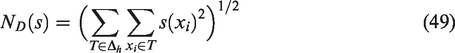
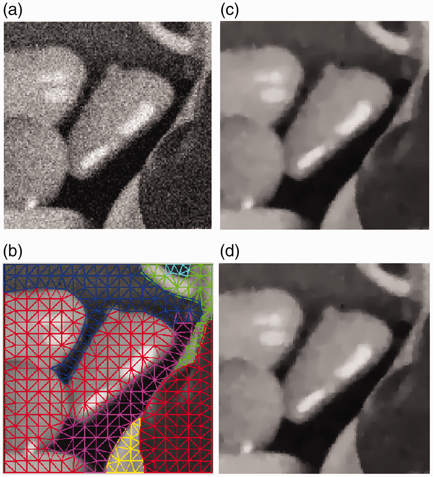
Experiment 3 (Denoising a natural image with an edge-adapted triangulation). We show that by using a triangulation that aligns with the edges in the image, we make our approach very competitive with the finite difference method as measured by peak signal-to-noise ratio, see Table 1. In this experiment, the MSA spline method is run separately on the regions identified by a segmentation of the image, see Figure 4 panel (b).

Figure 4.

(a) The image to be cleaned was obtained by addition of a sample from a white noise with σ = 20 onto the ground truth image in panel (b). (b) Edge adapted triangulation of the image domain. (c) Recovered image using the MSA spline approximation with ϵ = 1, d = 6 and r = 1. (d) Recovered image using Perona–Malik finite difference denoising. Original MSA Bicubic Bilinear.

Table 1.

The PSNRs of various regions in Figure 4, Panel (b).

	Perona–Malik	MSA spline
Region 1 (red, left)	29.9161	29.9109
Region 2 (green)	28.8445	28.9952
Region 3 (yellow)	31.6307	31.6989
Region 4 (purple)	33.0744	33.1167
Region 5 (blue)	33.3464	33.5832
Region 6 (red, right)	32.4490	32.5882

Experiment 4 (Total variation image resizing). Image resizing consists in increasing/decreasing the resolution of a given digital image. We achieve this easily by fitting a spline function to the available image using (50) and evaluating the resulting spline over the pixel locations for the new resolution of the image. We illustrate this approach with two examples in Figure 5; each image in the first column is resized by a factor of 10, that is, the resulting images have 10 times more pixels along each direction that the original images. The first original image is of dimension 18 × 28 pixels, while the second one has a resolution of 15 × 24 pixels. One can notice that both the bicubic and bilinear interpolation methods lead to the Gibbs discontinuity effect at the edges of the two images, while our approach barely show any such effect.

Figure 5.

Two images are scaled by a factor of 10 using the MSA spline method with d = 7 and r = 1. The results are compared to the bicubic and bilinear interpolation methods implemented in the MATLAB®’s function imresize.⁵³