Frequency estimator by combination of phase difference method and interpolation algorithm

Abstract

In the traditional time-shifting based phase difference method, considerable errors may be introduced by wrapped phase problem as long as translation coefficient tends to one even in a small-scale turbulence noise. In this paper, an improved frequency estimator is proposed to overcome the problem of wrapped phase by combination of phase difference method and interpolation algorithm. Compared with the traditional method of phase difference based on time-shifting, the improved algorithm can obtain an accurate estimate when translation coefficient exceeds one. Comparative studies were done by means of root-mean-square error over Cramer–Rao lower bound. According to the computer simulations, it is demonstrated that root-mean-square errors can cross Cramer–Rao lower bound if the translation coefficient is properly selected even in the case of the low signal-to-noise ratio, which implies that the proposed algorithm has a strong noise immunity. Finally, the advantage of the proposed algorithm is illustrated for the simulation signal which contained strong local random noise.

Introduction

Phase difference method and interpolation algorithm are two of effective spectrum correction techniques to reduce the bias caused by the non-integer period sampling. ¹ The interpolation-based method, in which the frequency error can be corrected by the ratio of a certain number of known discrete Fourier transform (DFT) spectral bins, has the advantage of low computational burden.^2–9 Early in 1970s, the interpolation algorithm, based on the modulus of two DFT bins, was proposed by Rife and Vincent. ² In the following decades, various improved algorithms were presented, such as the multi-point interpolated DFT approach, ³ the weighted interpolation approach.^4–6 However, most of the interpolation algorithms were established on the specific window or a cluster of windows. In 2015, Candan ⁷ proposed a frequency estimator by calculating the correcting factor of window function ⁷ to break the limit of window choice. At the same time, Luo et al.^8,9 investigated the interpolation algorithms for classic windows based on main-lobe fitting technique and zero padding technique. In contrast, the phase difference method is feasible for all kinds of windows and can be implemented conveniently without calculating any parameters in advance. As a result, it is extensively applied to various engineering fields, such as vibration monitoring, ¹⁰ fault diagnosis,^11–13 coriolis mass flowmeter,^14,15 power electronic parameter estimation ¹⁶ and so on.

The phase interpolation estimator (PIE) method was firstly proposed by McMahon et al. ¹⁷ to estimate the frequency. In 1994, the leakage-induced phase error was researched through analyzing the windowing signal. ¹⁸ In 2002, an universal method of phase difference based on time-shifting (PDTS) was presented by Ding and Zhong, ¹⁹ in which the translation coefficient was less than or equal to 1. The algorithm proposed by Ding et al. ²⁰ was a special case of PDTS by employing two continuous segment signals. In the light of the translation of the window center, Huang and Xu ²¹ derived a new phase difference algorithm. Meanwhile, the synthesized phase difference method based on time-domain translation and the changing width of symmetrical window were put forward by Ding et al. In 2007, the estimation error of PDTS in the case of Gauss White noise was analyzed. ²³ By considering the effect from negative frequency, an algorithm for low-frequency vibration signal was provided by Zhang and Tu. ²⁴ Recently, McKilliam et al. ²⁵ deduced a phase unwrapping estimator in the least squares sense. In view of utilizing the peak DFT bins of sub-segment from input samples with N points, the phase difference method, which is similar to the PDTS, was derived. ²⁶ Simultaneously, the calculation burden and statistical properties were also investigated. What’s more, Luo et al. made full use of the phase characteristics of asymmetric window and presented a new phase difference method, which can gain precise frequency estimated value only from one signal segment. ¹

The time-shifting based phase difference method has many advantages. For example, as translation coefficient increases, the errors caused by random noise or other interference would be reduced, consequently enhancing the estimation accuracy. In particular, the method is also advantageous for sampled signal containing strong local noise. However, once the translation coefficient exceeds one, considerable estimation errors would appear in the case of a large frequency deviation because of wrapped phase problem. In this paper, we focus on this problem and try to establish an improved phase difference algorithm which can still work when the translation coefficient is more than one. The remaining structure of the paper is as follows, in the next section, the theoretical background is illustrated. The derivation of the improved phase difference based on time shifting is then described. The simulations and results can be found in the subsequent section. Finally, some conclusions are summarized in the last section.

Theoretical background

For simplicity but without losing the generality, we consider an exponential signal emerged in random white noise

$$x_0\left(n\right)=A{e}^{j(2\pi \frac{f_0}{f_s}n+{\theta }_0)}+z\left(n\right)n=0,1,\dots N-1$$

(1)

where A, $f_0$ , ${\theta }_0$ , $f_s$ , N represent the amplitude, theoretical frequency, initial phase, sample rate and the number of samples, respectively. The last term $z(n)$ denotes the Gauss White noise, in which the mean is zero and variance is ${\sigma }^2$ . If the normalized frequency is described as ${\lambda }_0$ , and frequency resolution is expressed as $\text{Δ}f$ , the relationship can be obtained

$${\lambda }_0=\frac{f_0}{\Delta f}=\frac{f_0}{f_s/N}$$

(2)

At this stage, we ignore the noise term in the following part. After multiplying the time-shifting window function $w_N(n)$ to the exponential signal in equation (1), the weighted samples can be written as

$$x_w{\hspace{0.17em}}_0(n)=x_0(n)w_N(n)$$

(3)

where $w_N(n)$ can be achieved by

$$w_N(n)=w(n-N/2)$$

(4)

According to the convolution theorem, the DFT coefficients at spectrum line k of equation (3) can be calculated by

$$\begin{array}{c}{X}_{w0}(k)=A{W}_N(k-{\lambda }_0)e^{j{\theta }_0}\\ =\mathit{AW}(k-{\lambda }_0)e^{j\left[{\theta }_0+\tau (k)\cdot ({\lambda }_0-k)\right]}0\le k\le N-1\end{array}$$

(5)

where $\tau (k)$ is the slope of phase for $w_N(n)$ at k-bin, and $W_N(\cdot )$ , $W(\cdot )$ denote the DFT coefficients of $w_N(n)$ and $w(n)$ , respectively. In general, ${\lambda }_0$ lies between two DFT bins due to non-integer sampling. Therefore, ${\lambda }_0$ can be further described as

$${\lambda }_0=m+\delta$$

(6)

where m is the integer part which can be rapidly located with its maximum peak of signal in frequency domain, and $\delta$ ( $-0.5\le \delta \le 0.5$ ) is the fractional part of ${\lambda }_0$ .

Classic interpolation method

Subscribing equation (6) into equation (5) and replacing k by $m$ , the highest amplitude can be given by

$$\left|X_{w0}\left(m\right)\right|=A\left|W\left(-\delta \right)\right|$$

(7a)

Similarly, the second highest amplitude can be written as

$$\left|X_{w0}\left(m\pm 1\right)\right|=A\left|W\left(-\delta \pm 1\right)\right|$$

(7b)

In two-point interpolation methods, the ratio of two highest amplitude is defined as

$$\alpha =\frac{\left|X_{w0}(m\pm 1)\right|}{\left|X_{w0}(m)\right|}=\frac{\left|W(-\delta \pm 1)\right|}{\left|W(-\delta )\right|}$$

(8)

In terms of equation (8), the frequency bias can be described as a function of $\alpha$ related to window

$$\delta =g_w(\alpha )$$

(9)

It can be seen in equation (9) that frequency offset can be solely determined once the window is selected. For the maximum side-lobe decay (MSD) window, the relationship can be simply written as ⁵

$$\delta =\pm \frac{H\alpha -\left(H-1\right)}{\alpha +1}$$

(10)

where H is the number of terms in the MSD window, and the sign of $\delta$ can be determined by the second highest amplitude. ²⁸ For other windows, the polynomial approximation ⁶ or the iterative approximation ⁹ is suggested.

Phase difference method based on time-shifting

Compared with interpolation algorithm, the time-shifting based phase difference method requires two signal frames. The signal with M points delay of equation (1) is expressed as

$$x_1(n)=A{e}^{j(2\pi \frac{f_0}{f_s}n+2\pi \frac{f_0}{f_s}M+{\theta }_0)}n=0,1,\dots N-1$$

(11)

Similar to equation (3) and equation (5), the DFT coefficients of the weighted time-shifting signal can be described as

$$X_1(k)=\mathit{AW}(k-{\lambda }_0)e^{j[{\theta }_0+2\pi \frac{{\lambda }_0}{N}M+\tau (k)\cdot ({\lambda }_0-k)]}0\le k\le N-1$$

(12)

After substituting $m$ into equations (5) and (12), the phases for the two signal frames can be calculated by

$${\phi }_0(m)={\theta }_0+\tau (m)\cdot ({\lambda }_0-m)$$

(13a)

$$\text{ and }{\phi }_1(m)={\theta }_0+\tau (m)\cdot ({\lambda }_0-m)+2\pi (m+\delta )S$$

(13b)

In equation (13b), $S=M/N$ is the translation coefficient. Since the period of phase is $2\pi$ , the phase obtained through DFT is the main value of original phase. If we define the phases calculated from DFT as ${\varphi }_0$ and ${\varphi }_1$ , respectively, the phase difference $\Delta \phi$ can be established as

$$\text{Δ}\phi ={\varphi }_1-{\varphi }_0=\left\{{\phi }_1(m)-{\phi }_0(m)\right\}=\left\{2\pi \mathit{mS}+2\pi \delta S\right\}$$

(14)

where { $\cdot$ } denotes implementing $2\pi$ modulo operation.

Let us define $\text{Δ}\overline{\phi }=\{\text{Δ}\phi -2\pi \mathit{mS}\}$ . Since the phase belongs to the range $(-\pi ,\pi )$ , $\Delta \overline{\phi }$ may exceed the range $(-\pi ,\pi )$ . To guarantee the range of phase difference and frequency offset corrected by PDTS, the following operation is required

$$\Delta \overline{\phi }=\{\begin{array}{cc}\Delta \overline{\phi }-2\pi & \Delta \overline{\phi }>\pi \\ \Delta \overline{\phi }+2\pi & \Delta \overline{\phi }<-\pi \end{array}$$

(15)

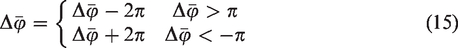
For the traditional PDTS, the translation coefficient is less than 1, equation (14) can be further simplified as (see Appendix 1)

$$\text{Δ}\overline{\phi }=2\pi \delta S$$

(16)

As a result, the frequency offset can be expressed as

$$\delta =\frac{\text{Δ}\overline{\phi }}{2\pi S}$$

(17)

Finally, the frequency estimate can be calculated by

$$f_0=(m+\delta )\cdot \Delta f$$

(18)

Derivation of the improved algorithm

It is known from ‘Phase difference method based on time-shifting’ section that the traditional PDTS is built on ignoring the phase ambiguity while translation coefficient is less than 1. However, phase ambiguity is supposed to be taken into account once translation coefficient is equal to or beyond 1. Considering the phase ambiguity and the noise interference on frequency estimator, frequency error corrected by PDTS should be rewritten as (see Appendix 1)

$$\widehat{\delta }=\frac{\Delta \phi +2\pi l-2\pi \mathit{mS}+Z_n}{2\pi S}=\frac{\Delta \phi +2\pi l-2\pi \mathit{mS}}{2\pi S}+\frac{Z_n}{2\pi S}$$

(19)

where l is the number of phase wrapping and $Z_n$ is the noise term in frequency domain.

As illustrated in equation (19), the influence of noise term would be reduced and would approach with the increasing translation coefficient, and hence the estimation value would be more precise. However, the number of wrapped phase cannot be known according to translation coefficient in advance, so the effectively corrected range of traditional PDTS would be shrunk as the increasing translation coefficient. To guarantee the feasibility of PDTS using equation (16) while translation coefficient is larger than one, it is necessary to add a correction value of high accuracy which can ensure the residual bias to meet the requirement in equation (32) (Appendix 1). The initial correction value can be achieved in the absence of noise and approximately obtained as much as possible in the presence of noise by the interpolation method (simplified as Selva) proposed in Selva. ²⁹ First of all, we employed, respectively, Selva algorithm to estimate frequency from signal $x_w{\hspace{0.17em}}_0(n),x_{w}1(n)$ . Subsequently, two estimated values of frequency can be obtained, and are defined as ${\lambda }_1$ and ${\lambda }_2$ . There are a set of mean values in statistics, such as arithmetic mean value, geometric mean value, harmonic mean value, and the quadratic mean value. In this paper, we take the arithmetic mean operation to reduce the random error of initial estimate and define $\overline{\lambda }$ as arithmetic mean. $\overline{\lambda }$ can be given by equation (20).

$$\overline{\lambda }=\frac{{\lambda }_1+{\lambda }_2}{2}$$

(20)

Replacing m with $\overline{\lambda }$ in equation (14), and expressing the bias addressed by the improved PDTS as $\overline{\delta }$ , the final estimate of normalized frequency can be computed by

$$\widehat{\lambda }=\overline{\lambda }+\overline{\delta }$$

(21)

At last, the improved PDTS can be summarized as follows:

Two discrete signals $x_0(n)$ and $x_1(n)=x_0(n+M)$ with N samples are acquired.

Obtain the tappered sequences $x_w{\hspace{0.17em}}_0(n)=x_0(n)w_N(n)$ and $x_{w}1(n)=x_1(n)w_N(n)$ , where $w_N(n)$ is the adopted window function.

Estimate the coarse frequency estimates ${\lambda }_1$ and ${\lambda }_2$ , respectively, from $x_w{\hspace{0.17em}}_0(n)$ and $x_{w}1(n)$ by Selva method.

Compute the arithmetic mean by $\overline{\lambda }=({\lambda }_1+{\lambda }_2)/2$ .

Calculate the phase difference $\Delta \phi =\arg \left[Y_1(\overline{\lambda })\right]-\arg \left[Y_0(\overline{\lambda })\right]$ , where $Y_1(\cdot )$ and $Y_0(\cdot )$ are the DFT coefficients of $x_{w}1(n)$ and $x_w{\hspace{0.17em}}_0(n)$ , respectively.

Return the bias by $\overline{\delta }=\Delta \overline{\phi }/2\pi S$ , where $\text{Δ}\overline{\phi }=\left\{\text{Δ}\phi -2\pi \overline{\lambda }S\right\}$ and $S=M/N$ .

The final frequency estimate is expressed as $\widehat{f}=\left(\overline{\lambda }+\overline{\delta }\right)\cdot \Delta f$ .

Simulations and results

Performance of the improved algorithm without noise

In this section, the comparative study between traditional PDTS and improved PDTS is investigated in the case of noiselessness. For convenience but without losing the generality, the sample rate and the number of samples were set as 256, which implied the frequency resolution was equal to 1. The theoretical frequency and phase were varied from [63.5,64.5] with steps of 0.025 and $[-\pi ,\pi ]$ with steps of $\pi /20$ , respectively, and the translation coefficient was selected with 0.0625 interval in the range of [0.0625,4]. For different phases, the maximum absolute error of frequency was selected. Figure 1(a) and (b) depicts the curve of maximum absolute error corresponding to traditional PDTS and improved PDTS. As described in Figure 1(a), the maximum error introduced by wrapped phase problem in traditional PDTS is about 1 under noiseless situation, and it also exams equation (16) that the effectively corrected range of traditional PDTS is decreased (blue district in Figure 1(a)) with the increasing translation coefficient. Otherwise, Figure 1(b) reveals that the improved method can be described as a frequency estimator of high accuracy, because the maximum absolute errors are all below 10⁻¹³ for different frequency deviations and translation coefficients.

Figure 1.

Maximum absolute error of frequency versus $\delta$ when Hanning window is used. (a) Traditional PDTS (b) Improved PDTS.

Performance of the improved algorithm with random Gaussian noise

To verify the feasibility and robustness of improved algorithm in the case of random noise, following simulations are performed. The exponential signal corrupted by Gauss White noise was generated by equation (1). The ratio of root-mean-square error (RMSE) to Cramér–Rao lower bound (CRLB) was investigated to evaluate the behavior of the improved algorithm. The expressions of RMSE¹ and CRLB³⁰ can be calculated by

$$\text{RMSE}=\sqrt{\frac{1}{N_{\mathit{tr}}}\sum _{i=1}^{N_{\mathit{tr}}}{(f_i-f_0)}^2}$$

(22)

where $N_{\mathit{tr}}$ denotes the number of independent instances and $f_i$ denotes the estimation value of frequency for each independent instance

$$\text{CRLB}=\{\begin{array}{ll}\frac{6f_{s}2}{4{\pi }^{2}S\mathit{NR}\cdot \left(M+N\right)\cdot \left[{(M+N)}^2-1\right]}& S<1\\ \frac{6f_{s}2}{8{\pi }^{2}S\mathit{NR}\cdot N\cdot (4N^2-1)}& S\ge 1\end{array}$$

(23)

In equation (23), the SNR is defined as

$$\mathit{SNR}=10{\log }_{10}(A^2/{\sigma }^2)$$

(24)

Maximum translation coefficient

In this subsection, the maximum translation coefficient in the case of different SNRs (dB) is discussed. The theoretical frequency and initial phase were selected randomly in [63.5,64.5] and $[-\pi ,\pi ]$ , respectively. The translation coefficient was varied from 1 to 20 with steps of 1, and for each translation coefficient, a total of 10,000 instances were tested. Figure 2 depicts the ratio of RMSE to CRLB with different SNRs (dB) and window functions.

Figure 2.

Ratio of RMSE to CRLB versus S. (a) Rectangle window (b) Hanning window (c) Hamming window (d) Blackman window.

From the pictures, it should be pointed out that the performance trend is identical with regard to different SNRs when the translation coefficient is less than or equal to 4. In addition, it is obvious for all selected windows that the ratio curve initially declines as we add translation coefficient, then minimum value and starts to go up as the translation coefficient increases except the situation that the SNR =10. The point with maximum translation coefficient and minimum ratio value, which reflects the excellent capability of anti-noise, is different for variable SNR. The reason is that the improved method can only compensate the error caused by wrapped phase problem in certain extend. As the translation coefficient increases, the interference from noise on PDTS is deceased, and the accuracy is remarkably improved. For instance, the minimum ratio can approximately attach to 0.3, while SNR is equal to −5 dB. However, it should be stressed that the interpolation algorithm in Step 3 would suffer obstacle from noise disturbance if a low SNR is encountered. The problem may, in turn, lead to a considerable residual error ${\delta }_1$ , which is intended to be corrected by PDTS. Unfortunately, PDTS may not work because it is possible that ${\delta }_{1}S$ exceeds the effective range in equation (32). As a result, we have to make a careful balance between maximum translation coefficient and noise disturbance in practise.

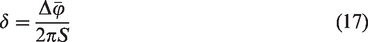
However, it is complicated to establish the relationship by theoretical derivation, so we attempt to zoom the simulation parameters to simulate the corresponding relationship between maximum translation coefficient and random noise. The parameters of theoretical frequency and phase were same as above. The SNR was varied from −5 dB to 15 dB with steps of 1 dB, and translation coefficient was varied from 0.25 to 20 with steps of 0.25. Figure 3 describes the ratio of RMSE to CRLB as a function of S and SNR for different windows.

Figure 3.

Ratio of RMSE to CRLB versus S and SNR (a) Rectangle window (b) Hanning window (c) Hamming window (d) Blackman window.

It is shown in pictures that the relationship is almost identical for different window techniques, because the capability to resolve the problem of wrapped phase is dependent on the accuracy of the interpolation algorithm. The phenomenon implies that the relationship between S and SNR can be obtained by curve fitting technique through one of selected windows. The result of curve fitting with rectangle window is depicted in Figure 4, and the formula for the relationship is established in equation (25). In Figure 4, it can be seen that the value of line-fitting is a little larger than data when the SNR is in the range of [1 dB,6 dB]. To guarantee the high accuracy with maximum translation coefficient calculated by the fitted expression, the floor function, where floor (·) denotes the nearest integers less than or equal to (·), should be operated. What’s more, it can also be known that the maximum translation coefficient can be attached to 20, while SNR is larger than 10 dB in equation (25), and at this time, the RMSE of improved method can be 0.07 times over CRLB.

$$S_{\text{max}}\approx \{\begin{array}{ll}\text{floor}\left(7.338\cdot e^{0.1114\cdot \mathit{SNR}}\right)& \mathit{SNR}<10\\ 20& \mathit{SNR}\ge 10\end{array}$$

(25)

Figure 4.

Line-fitting curve of S versus SNR.

Influence of frequency deviation

In order to assess the performance of the improved phase difference for changing deviations of frequency, we set theoretical frequency to vary with 0.05 interval in the range of [63.5,64.5] and SNR is equal to −5 dB. Initial phase was randomly selected in $[-\pi ,\pi ]$ and translation coefficient was selected separately as S = 1, S = 2, S = 3, S = 4. For different window functions, the performance of the improved method for different deviations is depicted in Figure 5.

Figure 5.

Ratio of RMSE and CRLB versus different deviations (a) Rectangle window (b) Hanning window (c) Hamming window (d) Blackman window.

From these pictures, it can be found that the trend of ratio curves is almost a uniform flat in the whole range of frequency deviations due to the first scheme corrected by interpolation method. ²⁹ The interpolation method can eliminate the effect for wrong location maximum spectral bins when frequency deviation is close to $\pm 0.5$ . Moreover, with the increase of S, the ratios are all reduced, and particularly, RMSEs can cross CRLB when S is larger than or equal to 2 for different window functions. The ratio of RMSE to CRLB can approximately reach 0.58, 0.67, 0.7, 0.75 corresponding to rectangle window, Hamming window, Hanning window and Blackman window supposing S = 2, and approximated equal to 0.3, 0.33, 0.35, 0.37 supposing S = 4. Thus, these features exam that the capability of noise immunity of the improved algorithm is independent on frequency deviations and can be enhanced with the increase of translation coefficient as shown in equation (19).

Algorithm analysis under simulated signal interfered by strong local random noise

In practical process of sampling, it is possible that the signal may be corrupted by strong local noise. In this subsection, the problem is considered to exam the advantages of the improved phase difference algorithm. At first, the Gauss White noise with zero mean was generated with SNR = −15 dB and −25 dB, respectively. In order to simulate well the real environment noise, the Kaiser–Bessel window ( $\beta =3.5$ ) was used to weight the noise to change the distribution of noise. For the sake of brevity, the basic simulation parameters are set as follows. The number of samples and sample rate was equal to 200, and the frequency deviation was scanned with 0.05 interval in [−0.5,0.5]. A total of 5N signal was generated with random phase. For example, the curve of simulated signal ( $\delta =0.5$ ) with different strong local noise can be found in Figure 6. Here, we compared the RMSE of the improved algorithm (rectangle window) and the interpolation algorithm in Selva ²⁹ (simplified as Selva).

Figure 6.

Simulation sampled signal when the additive noise is weighted by Kaiser–Bessel window ( $\beta =3.5$ ). (a) SNR = − 15 dB (b) SNR = − 25 dB.

In Figure 7(a) and (b), F_N and L_N denote the first segment signal and the last segment signal with N points, respectively. The RMSEs of two methods and arithmetic mean of estimation value are comprehensively compared. It can be seen that the RMSEs of Selva method with N points are not related to the F_N or L_N, and the operation, taking arithmetic mean, can reduce the random error caused by noise. For the two kinds of signal frames, the RMSE of improved algorithm is approximately 0.02 times over Selva (5N) in Figure 7(a). It can be seen in Figure 7(b) that the RMSE even approximately attach to 28, which vertifies the Selva (5N) method has worst behavior due to the wrong location of maximum spectral bin. In contrast, the frequency corrected by the improved method always keeps the privilege than other frequency estimates. Consequently, it can be concluded that the improved PDTS can be a good strategy to achieve the precise estimation of frequency when samples are submerged by strong local random noise.

Figure 7.

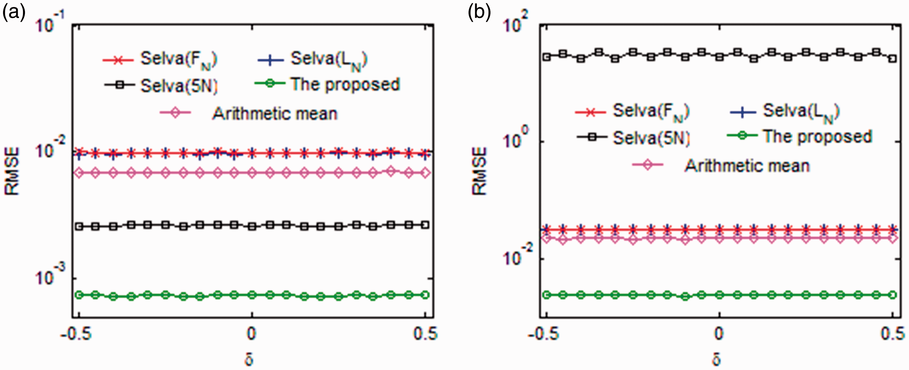
RMSEs of different estimation values versus deviations when the noise is weighted by Kaiser–Bessel window ( $\beta =3.5$ ). (a) SNR=−15 dB (b) SNR=−25 dB.

Conclusions

The paper illustrates a frequency estimator by combining the PDTS and interpolation algorithm to estimate frequency. The extensive simulation results verify the effectiveness of the proposed frequency estimator, and the improved method can be applied for several kinds of window functions. As the translation coefficient increases, the capability against random noise becomes stronger; in particular, the ratios of RMSE to CRLB can even approximately attach to 0.35 for different window functions when translation coefficient is equal to 4. For the sake of keeping the balance between maximum translation coefficient and random noise, curve fitting technique is used to obtain the arithmetic relationship. It can be known in equation (25) that the maximum translation coefficient can be 20 if SNR is equal to or larger than 10 dB and high precise estimate can be achieved. What’s more, while the stable samples interfered by strong local noise, which may be generated by sampling environment, the improved algorithm can still achieve high accuracy parameters estimation.