Ant colony optimisation of a community pharmacy dispensing process using Coloured Petri-Net simulation and UK pharmacy in-field data

Abstract

There are 11,619 community pharmacies in England which dispense over 1 billion prescriptions each year, providing essential primary care to NHS (National Health Service) patients. These pharmacies are facing pressure from a number of sources including funding cuts and high demands on services, while trying to deliver the highest standards of care. This paper presents an optimisation of a Coloured Petri Net (CPN) community pharmacy simulation model using an Ant Colony Optimisation (ACO) method. The CPN method was proposed by Naybour et al . Quantitative data from UK community pharmacies was collected by the authors and incorporated into the CPN simulation model. The optimisation is made up of a choice of how many staff to employ, which prescription checking strategy to use, and which staff work pattern to implement. This method aims to provide decision makers with a set of optimal pharmacy configurations at different cost levels. This can help to support pharmacy safety, efficiency, and improve decision making processes. It has been demonstrated how reliability modelling techniques traditionally used in safety-critical industries, can be used to carry out safety and efficiency analyses of healthcare systems, such as dispensing processes in community pharmacies, illustrated in this contribution.

Introduction

Over the last two decades healthcare systems have become increasingly aware of patient safety issues occurring during the delivery of care. ¹ However, as well as being required to provide a safe and reliable service, it has been established that patient satisfaction with community pharmacy services is related to waiting times. ² These two fundamental objectives, delivering safe care, in an efficient manner, can come into conflict.

A recent study investigating the number of medication errors occurring in the National Health Service (NHS) estimated that 237 million errors occur each year, of which 15.9% are attributed to dispensing errors. ³ This paper contributes to a growing body of work^4,5 exploring how techniques more traditionally applied in high risk industries, such as the nuclear^6,7 or aviation sectors, ⁸ might be gainfully employed in healthcare contexts. It aims to provide a decision support tool to aid community pharmacy management and resourcing. Community pharmacy decision makers in the UK have less money to deliver a higher volume of services in a safer manner than has been done previously. This paper aims to address this problem by providing quantitative evaluations for the performance of different community pharmacy configurations, and by coupling those evaluations with a price, aiding decision makers when choosing how to staff community pharmacies.

Previous modelling

Healthcare has been the setting for a large number of simulation projects. ⁹ The literature demonstrates that community pharmacies have been the setting for a number of them. Projects that have focused on reliability aspects of dispensing have included: an FMEA project based in community pharmacies, ¹⁰ and a socio-technical probabilistic risk assessment (ST-PRA) of the community pharmacy dispensing process. ¹¹ For example, in the ST-PRA a modelling team constructed fault trees for 10 preventable adverse drug events involving six high risk medications. Projects have also focused on analysing pharmacy efficiency. These have included: a discrete event simulation model used to evaluate the impact on waiting times made by the use of an automated dispensing machine, ¹² and a multiple server model based on queueing theory which involved varying the number of staff and comparing the resulting waiting time for patients. ¹³ Markov models have been used to optimise the replenishment process of robotic dispensing systems, ¹⁴ as well as to evaluate the cost effectiveness of healthcare interventions. ¹⁵ Other work has focused on maintaining inventories and resource allocation. Examples have included: an inventory control model for maintaining levels of medicinal products, ¹⁶ and a Petri net based methodology, MedPRO, designed to address organisation problems within healthcare systems. ¹⁷

Previous work of the authors has included developing a CPN simulation model of community pharmacies,^18,19 capable of evaluating both pharmacy reliability and efficiency in the same model. The CPN has a set of input variables, including the number and skill unit of staff, checking strategies, and work patterns, which produce different outcomes. This model takes account of in-field data collected by the authors, and is used within the optimisation framework proposed in this paper, in order to evaluate different pharmacy set ups. Section 2 introduces the CPN model used.

Optimisation method

Once the CPN simulation model of a pharmacy was constructed, the question arose of how best to set up the pharmacy. This is a multi variable optimisation problem. Rather than approaching the problem with an exhaustive search, it is more computationally efficient to use an algorithm.

This paper applies the Min-Max Ant System (MMAS) ant colony optimisation algorithm ²⁰ to a community pharmacy Coloured Petri Net simulation model. MMAS is an extension of the original Ant System algorithm developed by Dorigo et al. in 1991. Other extensions of the Ant System developed since the introduction of the original Ant System method have included best-worst Ant System, ²¹ elitist Ant System, and the Hyper-cube Ant System. ²² MMAS was chosen as the optimisation algorithm because this algorithm extension has been seen to produce accurate results when compared against other ant colony optimisation algorithms, for a detailed introduction to ACO and some of its key variants, including MMAS, see Dorigo et al. ²³

Ant Colony Optimisation is a meta-heuristic optimisation method, derived from the positive feedback aspects of biological ant behaviour. Example applications in the healthcare sector have included using simulated annealing, ²⁴ the tabu search, ²⁵ or genetic algorithms ²⁶ to optimise hospital units, and ACO algorithms have been used to optimise diabetes screening policies ²⁷ and emergency department efficiency. ²⁸ Meta-heuristic techniques also see application in a wide range of non medical fields. Examples have included using ACO to predict appropriate credit ratings for businesses, ²⁹ and the examination timetabling problem. ³⁰ ACO has been chosen as the optimisation algorithm in this paper as it is has performed well on discrete space optimisation problems. ³¹ There are other meta-heuristic algorithms that could potentially be used to solve the problem. The following algorithms have been used in the literature to optimise pharmacy related operations, and would also be candidates for solving the pharmacy dispensing problem: genetic algorithm, ³² simulated annealing, ³³ particle swarm optimisation, ³⁴ among others.

One characteristic issue with using HDN (Heuristics Defined in Nature), ³¹ is that their performance is controlled by a set of user determined parameters, and finding good values for these parameters can represent a whole new optimisation problem in itself. ³⁵ There are several approaches one can take to set the parameters. These have previously included: ad-hoc selection, ³⁶ utilising recommendations from previous research, ³⁷ or using experiments to identify optimum parameter settings.^38,39 One issue with using parameters that have performed well in previous studies is that the parameters can be very sensitive to the specific problem domain. This paper uses a semi-fixed set of parameters, similar to those seen in Stützle and Hoos ²⁰ and a heuristic inversion method of searching for optimal solutions is proposed.

This paper offers three novel contributions, which are as follows: the collection and distribution fitting analysis of in-field data, an extension of previous work by the authors in modelling community pharmacies by the inclusion of an optimisation framework, and the development of a novel three stage heuristic inversion method of ant colony exploration. It also aims to demonstrate how system reliability modelling and assessment methods, commonly used for the analysis of industrial systems, can have potential benefits for the analysis of reliability and efficiency of healthcare processes. ⁴⁰

The paper is structured as follows. Section 2 gives an outline of how the CPN model used to simulate the outcomes of different pharmacy scenarios was constructed. Section 3 presents the results of a data collection study carried out in 4 UK community pharmacies. Section 4 gives a description of the biological basis of the technique, before introducing the core mechanisms and equations proposed and used in the ACO algorithm. Section 5 details the optimisation problem, and how the MMAS algorithm has been applied to the particular state space, generated by the pharmacy simulation model. Section 6 presents the results of the MMAS optimisation, including a comparison with an exhaustive search, and Section 7 concludes the paper.

CPN modelling approach

This section starts with an overview of the dispensing process, then presents a short introduction to Petri Nets, and demonstrates how a Coloured Petri Net (CPN) model for simulating the processes carried out in a community pharmacy was developed. Note that tokens mimic the behaviour of pharmacy staff as they dispense prescriptions, and complete non-dispensing tasks. The CPN model is populated with transitions derived from in field data collection, and is then used to develop a community pharmacy optimisation problem.

The main stages of dispensing

A brief overview of the community pharmacy dispensing process is now presented. The six keys stages of the dispensing process are shown in their chronological order (in practice generating labels, and picking medicines can be interchanged) in Figure 1.^41–43 Prescriptions begin moving through the pharmacy after being handed in, either in person or electronically. After being handed in, a legal check is undertaken before a prescription will be dispensed. The labels detailing instructions for safe use are printed, and all items contained in the prescriptions are collected. The labels are adhered to the medicine boxes and when the assembly is complete, the finished prescription is given to a pharmacist or suitably qualified ACT (accredited checking technician), who performs a final accuracy check. This is the last chance for any errors incurred throughout the process to be caught and rectified. Any errors that are not caught at this stage are liable to be passed onto patients. As well as the accuracy check, a clinical check is performed on the prescription to ensure the medicine being dispensed is clinically suitable. Completed and checked prescriptions are then handed over to patients, or stored so they can be sent out for delivery, or picked up by patients later in the day.

Figure 1.

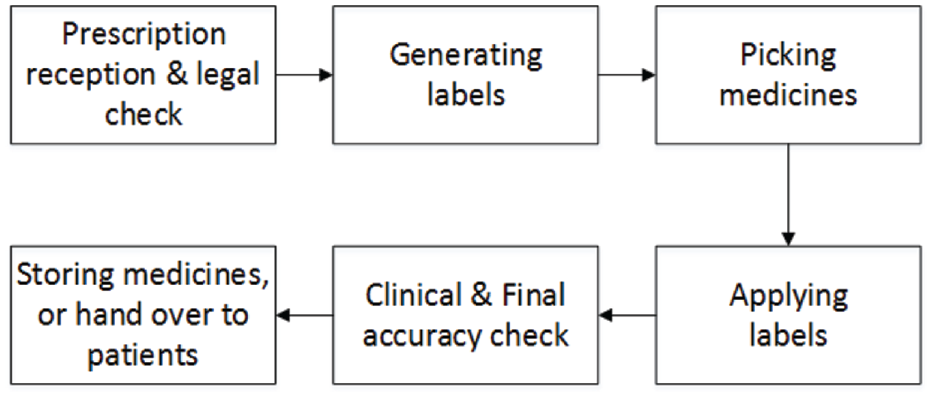
Dispensing process flow chart.

Petri Nets

Petri nets are a type of executable graph. They are made of a set of directed edges running between two sets of nodes, places and transitions. Arcs run between these two sets of nodes, but no arc will connect two places within the same set. Places contain a number of tokens, which are used to control transitions, following a firing rule. The CPN used as the basis of this optimisation uses a Timed Petri Net extension, where delay times can be sampled using specific probability distributions, or use deterministic delays time (also equal to 0). ⁴⁴ The Petri Net developed loosely follows the Stochastic Petri Net (SPN) formalism used in Bause and Kritzinger, ⁴⁵ although it differs in that it is not limited to only using exponential distributions for delays, and non-zero deterministic delays are allowed. If transition delay timings are restricted to exponential distributions, then Markov methods can be used to analyse Petri nets, otherwise, Monte Carlo simulations are used to derive results. The Petri net in this paper is not restricted to only using exponential distributions to control transition timings, so Monte Carlo methods are used to derive results.

Introduction to coloured Petri nets

Including colours in a Petri net framework enables for a more detailed analysis of token behaviour. Colours enable each token to represent distinct entities, unlike a Petri net without colours, where tokens on a single place are indistinguishable. This is useful because, we can use colours to track how staff tokens spend their time, and information about prescriptions can be encoded using colours. In this paper two colour sets, along with the basic token type (no colours), are used to define three types of token, prescription tokens (p), worker tokens (w), and basic tokens (e). The prescription token type has a number of colours, where each colour represents a feature of the prescription. The Coloured Petri Net framework was chosen because CPN models allow for simulating the efficiency and safety of a pharmacy within a single modelling framework, instead of having to develop separate models. The following features of prescriptions were modelled using colours:

1. The time taken to dispense the prescription

2. Delivery or a walk-in.

3. Number of iterations to complete the prescription, if faults occur (represents near misses)

4. The overall outcome of the prescription (near miss, dispensing error, or com-pletely correct)

5. The number of items in the prescription

6. Contents

7. Labels

8. Label application

Worker tokens use one colour to distinguish between the two roles modelled (pharmacist or dispenser), and another to define the tasks they are qualified to complete. The CPN makes use of basic tokens, which have no colours attached, for a number of auxiliary functions. These included, permanently enabling transitions, counting how many times advanced services were completed, and modelling the availability of labelling computers.

The firing rule for Coloured Petri nets is more complex than that of non-coloured nets, because there are extra control mechanisms, such as transition guard expressions and arc inscriptions to consider. Arc inscriptions specify which colour tokens are placed onto output places, and conversely, which colour tokens are required to enable a transition. Colours are used in this paper in a similar way to that seen in Jensen, ⁴⁶ and time is introduced following the method seen in Winfrid. ⁴⁴ An example CPN transition is shown in Figure 2. The marking next to each place describes the tokens within each place, and arc weights are written as a multi-set of token colours. For example, in place p2, there is one token of type e (denoted as 1’e) and two tokens of type p (denoted as 2’p). There are three token types in this example: p, w, and e. The colours on w tokens record the amount of time spent completing different task types, p tokens include a set of colours corresponding to the properties of prescriptions, and e tokens are basic tokens which have no colours. Once the transition has fired, the colours corresponding to waiting time and time spent completing activities are both increased by the delay time. In addition, a number of tokens is taken out of input places (such as one token of type p and one token of type e is taken out of place p2, as described on the arc by (y) + e; also note that variable y is of type p). A number of tokens is placed into the output places (such as one token of type w and one token of type p is placed in p4, as described on the arc by (x) + (y); note that variable x is of type w).

Figure 2.

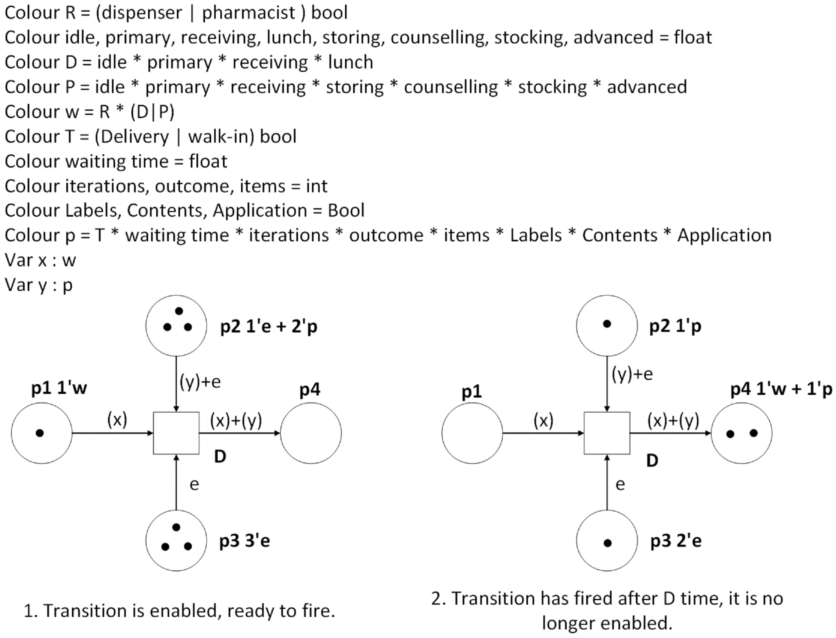
A coloured Petri net transition.

Building the model

The model used as the basis of this optimisation simulates a community pharmacy using a manual dispensing method (rather than automated dispensing ⁴⁷ ). It can accommodate varying numbers of pharmacists and dispensers, and staff are capable of working in parallel to complete prescriptions. Figure 3 shows the full graph of the CPN model. It was built by considering the journey of a single prescription through a pharmacy, from patient arrival to final handover of medicine, and integrating the way resources are used throughout the process. A detailed description of the meaning of all places and transitions in the CPN can be found in Naybour et al. ¹⁸

Figure 3.

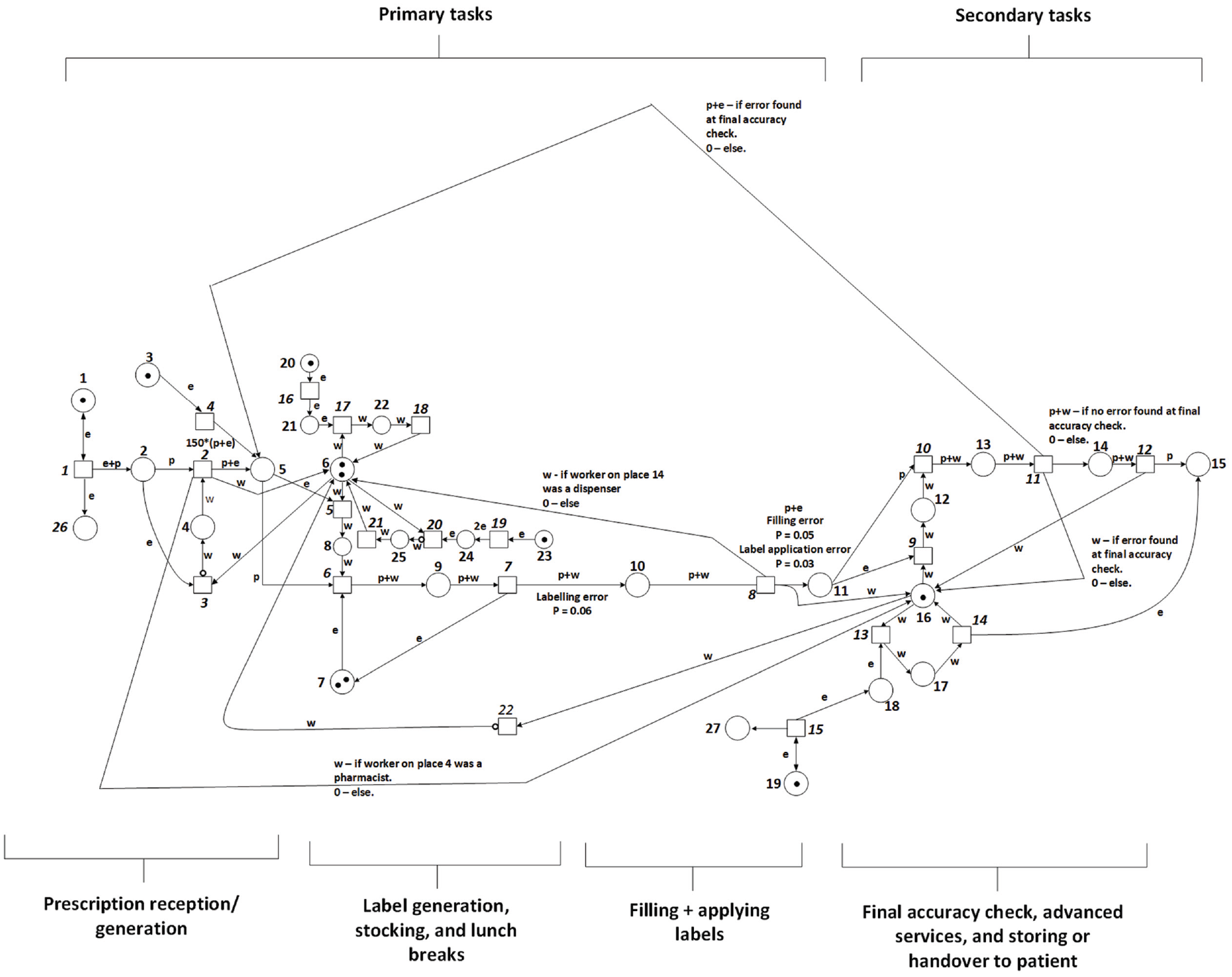
A coloured Petri net for modelling community pharmacy dispensing.

Modelling assumptions

To illustrate the level of detail in the model, the follow assumptions are described in this section. Each type of task is designated as being either a primary or a secondary task. Figure 4 shows that the model operates with a major distinction between primary and secondary tasks. Secondary tasks may only be completed by a qualified pharmacist, while primary tasks may be completed by any member of staff. As well as this feature, additional assumptions on how staff behave and how resources are utilised in the pharmacy are used. These are the assumptions used to control staff behaviour:

• The following tasks are classified as primary: stock management, generating labels, assembling prescriptions, applying labels, and receiving prescriptions.

• These tasks are classified as secondary, and may only be completed by pharmacists: carrying out advanced services, final accuracy checking prescriptions, passing completed prescriptions to patients and placing completed prescriptions in storage.

• Each staff member has the same level of competence and skill. That is they take similar amounts of time to complete tasks, and the chance that they will make an errors is the same.

• Pharmacist members of staff will complete primary tasks only if there are no secondary tasks waiting to be completed.

Figure 4.

Example ACO configuration.

This is the set of assumptions made about the pharmacies’ resources, opening hours and prescriptions:

• The pharmacy uses two labelling stations (small printers attached to computer interfaces which are used for printing labels).

• Patients arriving the pharmacy to hand in new prescriptions are prioritised as the highest priority primary task.

• The three stages, generating labels, assembling prescriptions, and applying labels, are completed sequentially by the same member of staff.

• Priority is given to walk-in prescriptions over deliveries.

• The pharmacy opens at 9 am and closes at 5 pm.

• A bulk of delivery prescriptions arrive at the pharmacy at 10 am.

Pharmacy resources

Initially, all pharmacist tokens are placed in place 16, and all dispensers are placed in place 6. New walk in prescriptions and customers requiring advanced services are introduced to the pharmacy by increments of exponential distributions. The two labelling stations are modelled by the basic tokens on place 7.

Primary task allocation

As new tasks arrive, members of staff are allocated to complete them. The member of staff that has been inactive on the ‘available’ place for the longest amount of time is tasked with the newly arrived task.

Instantaneous transitions are used to control the priority of each task. These control how staff make decisions about which task to complete when there are multiple unattended tasks. The primary dispensing tasks are prioritised from lowest to highest priority is as follows: starting to dispense a prescription, stock management, lunch breaks and receiving prescriptions. Attending to patients waiting in the pharmacy for their prescription is given the highest priority. Next comes the relatively low frequency tasks, lunch breaks and stock management. These are given priority over starting to dispense prescriptions because if starting to dispense prescriptions was prioritised, staff might not be able to get away from the demands of dispensing.

Secondary task allocation

Pharmacists are allocated to secondary tasks from their available place (16). Secondary tasks are prioritised from lowest to highest priority as follows: final accuracy checking/other secondary dispensing tasks, and advanced services.

Prescription modelling

The model uses eight colours to model prescriptions:

1. Type of prescription, delivery/walk-in.

2. Waiting time to dispense the prescription

3. Iterations, that is the number of times a prescription is sent to be dispensed again after an error is found in it.

4. End result of the prescription, near miss, dispensing error, or completely correct.

5. Number of items

6. Labels

7. Contents

8. Label application

The number of iterations is a value indicating the number of times a prescription was intercepted at the final accuracy check and found to contain an error. They are representative of near misses. Boolean variables are used to model the labels, contents, and label application variables, where each variable indicates the presence/absence of an error of each type.

Failures

Bernoulli random variables are used to simulate members of staff committing accidental errors within the dispensing process. The pharmacy model has four fallible stages: label generation, prescription assembly, label application and the final accuracy check. Table 1 show the probability of error at each stage in the process, where the probabilities were found in Cohen et al. ¹¹ It is a modelling assumption that applying labels to completed prescriptions will be half as likely to fail as generating labels.

Table 1.

Error probability. ¹⁸

Task	Description	Probability (%)
1	Labelling	0.06
2	Filling	0.05
3	Label Application	0.03
4	Final Accuracy check	0.05

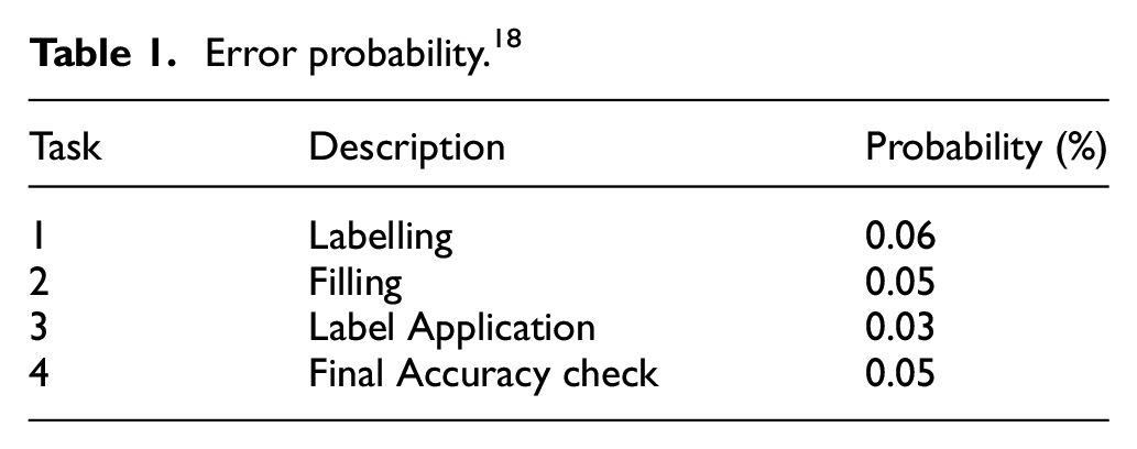
Arc inscriptions are used to allow for probabilistic failures of dispensing stages. A Bernoulli random variable is sampled as the transition representing the stage fires. If the value returned by the Bernoulli random variable exceeds the error probability in Table 1, then a colour will be added to the prescription token indicating which type of error has occurred.

Prescriptions arrive at the final accuracy checking stage of the process in a number of states. Some prescriptions will be completely correct, while others with contain one or more types of error. The model assumes that completely correct prescriptions are not incorrectly found to be erroneous at the final accuracy check. If a prescription contains an error at this stage, the pharmacist performing the check will spot errors, and send these prescriptions back to be dispensed again.

Item modelling

Prescriptions can contain a variable number of items. A large prescription might contain upwards of 15–20 items, while a small prescription can be only a single item. The model assigns each new prescription a random number of items by sampling a Geometric (0.35) distribution. The time to complete some stages of the dispensing process is then modulated by the number of items in prescriptions. Stages representative of processing tasks sample the timing distribution attached to their transition one time for each item in the prescription, these values are then summed to determine how long the process took.

Summary

This section has introduced the CPN model used to model a community pharmacy. Transitions of the CPN related to dispensing tasks are populated with probability distributions derived from our in-field data collection, see Section 3. This CPN is used in Section 4 as the basis for setting up a community pharmacy optimisation problem, where the number of staff, and differing checking strategies are used to create a state space for the optimisation. Further details of the model can be found in Naybour et al. ¹⁸

Data collection and analysis

To better inform the Coloured Petri Net simulation model developed in Naybour et al., ¹⁸ quantitative data of how long it takes to process prescriptions was collected from 4 UK pharmacies. Previous studies have attempted to time the dispensing process, although the sample sizes collected were small, ² or dispensing stages were not clearly distinguished. ⁴⁸

Fitting results

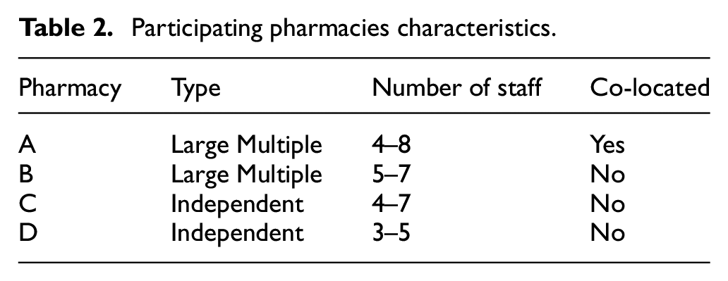
Table 2 shows key information about the four pharmacies which participated in the study. Pharmacies A and B were part of the same company, and pharmacies C and D were independent pharmacies. Being from the same company, pharmacies A and B shared the same set of standard operating procedures, ⁴² and there were therefore similarities in how medicines were dispensed in those two pharmacies. For the purpose of this paper the data collected from pharmacies A and B was grouped to create one larger data set for analysis. The data collected in pharmacies C and D were not used in this paper.

Table 2.

Participating pharmacies characteristics.

Pharmacy	Type	Number of staff	Co-located
A	Large Multiple	4–8	Yes
B	Large Multiple	5–7	No
C	Independent	4–7	No
D	Independent	3–5	No

Timing data was collected for six stages of the dispensing process shown in Figure 1. Through discussions with expert pharmacists, it was hypothesised that the middle four stages would be dependent on the number of items in a prescription, and the rest of the stages (reception and handover) would not be. Stages which are dependent on the number of items (i.e. stages 2, 3, 4 and 5) will be referred to as ‘processor’ stages. For the two non-processor stages 160 observations of a single variable were collected (the time taken to complete the stage), whereas for the processor stages, the data took the form of 160 observations of two variables:

1. The time taken to complete the stage

2. The number of items in the prescription

The data collection technique used was researcher observation, with a stopwatch used to time each stage. The data collection period was between 3 and 5 days at each pharmacy. After collection, the timing data for the processor stages was segmented into six categories: 1 item, 2 items, 3 items, 4 items, 5–8 items (medium), and 9+ items (large). Distribution fitting analysis was then performed on each of the non-processor stages, and each segment of each processor stage. A statistical package in R was used to test six probability distributions for each segment, using the method of maximum likelihood. ⁴⁹ We fit six probability distributions to the data: exponential, normal, lognormal, uniform, Weibull and gamma. For each fitted distribution (apart from the uniform distribution) an Akike Information Criterion value was calculated, where the distribution which produced the lowest AIC value was chosen. QQ plots for each distribution were used as a checking tool to see whether the result produced by the distribution fitting analysis aligns with the Q-Q plots. Finally, a bootstrap sampling method ⁵⁰ was used to derive 95% confidence interval for the estimated parameters. Table 3 presents the results of the distribution fitting analysis. Further details of the data collection and analysis can be found in Matthew et al. ⁵¹

Table 3.

Summary of distribution fitting analysis.

Task	No# items	Observations	Mean	Distribution	Parameter 1	Parameter 2
Prescription reception	N/a	160	17.9	X ∼ Gamma(α, β)	2.46	7.25
Label generation	1	150	27.2	X ∼ lognormal(µ, σ)	3.14	0.549
	2	57	38	X ∼ lognormal(µ, σ)	3.53	0.454
	3	33	54.6	X ∼ lognormal(µ, σ)	3.88	0.487
	4	36	59.5	X ∼ lognormal(µ, σ)	3.96	0.515
	Medium	34	90.8	X ∼ Gamma(α, β)	5.41	16.8
	Large	10	177.7	X ∼ Gamma(α, β)	4.48	39.7
Picking	1	138	18.7	X ∼ lognormal(µ, σ)	2.58	0.851
	2	65	20	X ∼ lognormal(µ, σ)	2.79	0.653
	3	38	27	X ∼ Gamma(α, β)	3.99	6.76
	4	27	45.7	X ∼ lognormal(µ, σ)	3.42	0.54
	Medium	43	56	X ∼ Gamma(α, β)	3.06	18.28
	Large	5	131.2	X ∼ Gamma(α, β)	4	32.8
Applying labels	1	113	19.2	X ∼ lognormal(µ, σ)	2.63	0.787
	2	68	32.3	X ∼ lognormal(µ, σ)	3.24	0.673
	3	30	40.8	X ∼ lognormal(µ, σ)	3.47	0.658
	4	30	50.8	X ∼ lognormal(µ, σ)	3.75	0.599
	Medium	61	91.5	X ∼ lognormal(µ, σ)	4.32	0.615
	Large	18	176.7	X ∼ Gamma(α, β)	2.59	68.5
Accuracy checking	1	133	32.2	X ∼ lognormal(µ, σ)	3.35	0.486
	2	68	45.2	X ∼ lognormal(µ, σ)	3.65	0.539
	3	34	59	X ∼ lognormal(µ, σ)	3.96	0.484
	4	34	47.9	X ∼ Gamma(α, β)	8.66	0.181
	Medium	50	83.4	X ∼ lognormal(µ, σ)	4.34	0.409
	Large	12	175.8	X ∼ lognormal(µ, σ)	4.97	0.629
Handover/store	N/a	160	34.2	X ∼ lognormal(µ, σ)	3.15	0.874

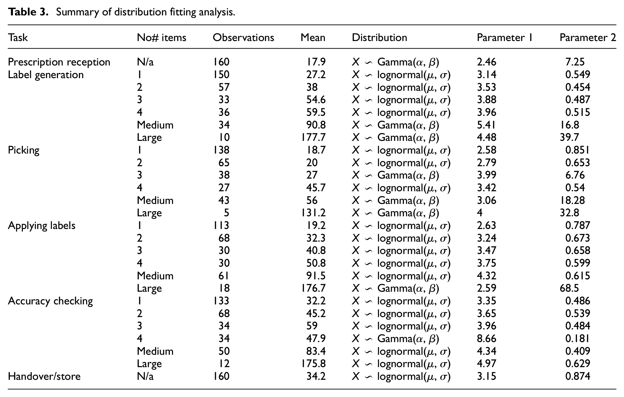
Extrapolation

For some of the segments, very few observations were collected (N < 15). In these cases, the distribution type was assumed to be the same as for medium sized prescriptions, with new parameters estimated based on any data that was collected for large sized prescriptions. Since large prescriptions made up less than 3.2% of prescriptions during simulations, this extrapolation should not have a large effect on the outcome of simulations using this assumption.

Ant colony optimisation

Laboratory experiments have been conducted by Goss et al. ⁵² and Deneubourg et al. ⁵³ demonstrating how ant colonies are capable of finding the shortest path to food sources using pheromones to guide the future behaviour of other ants. Each ant can communicate with other ants by secreting a pheromone trail of chemicals. As well as secreting the pheromone, every ant can also detect the trails of pheromone placed by other ants. The behaviour of collective path marking and path following, is the basis of Ant Colony Optimisation. Ant colony optimisation is known to be an effective algorithm for discrete optimisation problems. ³¹

Ant system

In ACO, artificial ants search the solution space of an optimisation problem, and ants which find good solutions to the problem then influence the future choices of the colony. Dorigo and Stutzle ⁵⁴ introduced the concept of Ant System to solve minimum path problems on graphs. Ant system has two main features: a solution construction decision policy, and a pheromone update strategy, which will be introduced, and later used to explain max-min ACO.

Ant system ants have two modes of operation, one for leaving the nest to travel to a food source (forward), and another one to return to the nest and lay pheromones (backward).

Solution construction

While in the forward mode, a number of ants simultaneously construct solutions on the graph by repeatedly applying a decision policy. The decision policy is probabilistic, and dependent on two factors: the amount of pheromone on edges connecting to neighbouring nodes, and the inherent desirability of each edge. Thus when an ant is on a node i, it uses the concentration of pheromone and some prior heuristic information about the edges, to probabilistically decide which node to move to next. If N_i is the set of nodes neighbouring node i, then an ant chooses the next node to visit, j, with probability p_ij. If the concentration of pheromone on paths from node i to all neighbouring nodes j are denoted by τ _ij , and the heuristic information about node j in relation to node i is ν _ij , then equation (1) describes the decision probability function:

$$p_{\mathrm{ij}}(t)=\{\begin{array}{c}\frac{{\left[{\tau }_{\mathrm{ij}}\right]}^{\alpha }{\left[{\nu }_{\mathrm{ij}}\right]}^{\beta }}{\sum _{l\in N_i}{\left[{\tau }_{\mathrm{il}}\right]}^{\alpha }{\left[{\nu }_{\mathrm{il}}\right]}^{\beta }}\mathrm{if}j\in N_i\hfill \\ \multicolumn{1}{c}{0,\mathrm{if}j\notin N_i}\end{array}$$

(1)

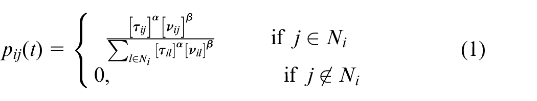
where p_ij(t) is the probability that an ant on node i at time t moves to node j as its next node. N_i, the neighbourhood of node i, is defined as the set of nodes which can be reached from node i by travelling along one edge, except for the node that was previously visited by the ant. The two parameters α and β control the relative importance given to pheromone or heuristic information in the decision policy. Ants move from node to node, using this decision policy to choose where to move next, until they have constructed a solution to the optimisation problem.

Variable heuristic search

It is common for MMAS algorithms to use a heuristic to encourage ants to search solutions with a lower cost value. ⁵⁴ This paper proposes a novel method of using heuristics to generate a larger set of optimal solutions. Rather than running a single iteration of the algorithm with a constant set of heuristic values, the algorithm will be run in three iterations.

At the start of each iteration, the pheromone trails on the state space from the previous iteration are cleared, and the heuristic values used by the ants are changed. The three underlying heuristics are as follows.

1. No heuristic values

2. A heuristic preferring low cost solutions

3. A heuristic preferring high cost solutions

Using the variable heuristic values will encourage ants to concentrate to explore different parts of the state space.

Pheromone update

After all ants have constructed their solutions, the pheromone values of all paths are then updated. This is done in two stages: first by reducing the concentration of pheromone on all arcs by the constant factor ρ, as in equation (2):

$${\tau }_{\mathrm{ij}}\leftarrow {\tau }_{\mathrm{ij}}(1-\rho )$$

(2)

and, then adding additional pheromone to arcs used by the ants, as in equation (3):

$${\tau }_{\mathrm{ij}}\leftarrow {\tau }_{\mathrm{ij}}+\Delta {\tau }_{\mathrm{k}}$$

(3)

where Δτ_ij k is the amount of pheromone deposited by the kth ant on the edge (i, j). Δτ _ij ^k is proportional to the quality of the solution generated by the kth ant, and it is calculated using equation (4):

$$\Delta {\tau }_k=\{\begin{array}{c}1/O^k\mathrm{if}(i,j)\in P_k\hfill \\ \multicolumn{1}{c}{0\mathrm{if}(i,j)\notin P_k}\end{array}$$

(4)

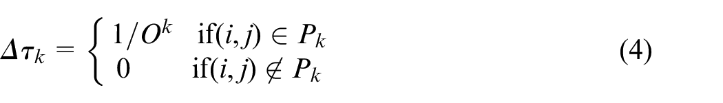
P_k is the set of edges used by the kth ant, and O^k is the objective value returned by the kth ant. If an ant chooses to use an arc (i, j) in its path to the food source, the deposit of pheromone onto the edge makes it more likely that future ants will also choose to use this arc to construct solutions. The structure of equation (4) also shows how ants which find better solutions will deposit more pheromone onto edges than those that find weaker solutions.

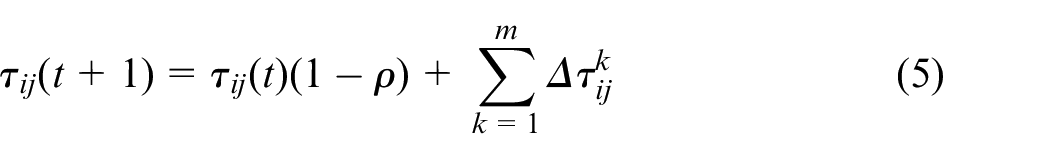
If there are m ants in the colony constructing paths and laying pheromone, then the concentration of pheromone on an edge (i, j) in the next iteration of the algorithm can be updated using equation (5).

$${\tau }_{\mathrm{ij}}(t+1)={\tau }_{\mathrm{ij}}(t)(1-\rho )+\sum _{k=1}^m\Delta {\tau }_{\mathrm{ij}}^k$$

(5)

Max-Min Ant System

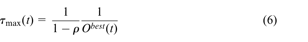
Max-min Ant System (MMAS) is an ACO variant developed by Stützle and Hoos, ²⁰ as a way to improve the algorithm’s performance by preventing early convergence to sub-optimal solutions. The key principle of MMAS, is to generate flexible bounds on the pheromone concentrations, so that the concentration on all paths is within some factor of the most marked path. This results in a more exploratory algorithm, since every edge is guaranteed a minimum probability of being selected. The Max-Min pheromone update follows equations (2)–(4), although only the global best ant, or the iteration best ant, are allowed to deposit pheromone onto the search space. Furthermore, pheromone trails are limited to an interval of values [τ_min(t),τ_max(t)]. If during the process, the pheromone trail on a path would be outside the boundary, it is instead set to the nearest bound. It can be shown that the maximum concentration of pheromone on a path is bounded by (1/1−ρ)*(1/O_best). In MMAS this guides the choice of τ_max, which is given in equation (6):

$${\tau }_{max}(t)=\frac{1}{1-\rho }\frac{1}{O^{\mathrm{best}}(t)}$$

(6)

Equation (7) shows how τ min is calculated:

$${\tau }_{min}(t)=\frac{{\tau }_{max}(t)(1-\sqrt[n]{p_{\mathrm{bset}}})}{(\mathrm{avg}-1)\sqrt[n]{p_{\mathrm{bset}}}}$$

(7)

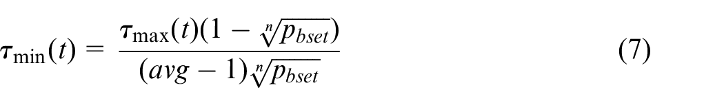
where p best is the probability that an ant will choose the maximally marked path once the algorithm has converged, and avg is the average number of choices an ant has at each step of the algorithm.

Application of MMAS to the pharmacy optimisation problem

In the UK, a community pharmacy is generally a small store focused on the provision of prescriptions to members of the public. The process of dispensing can be separated into six key stages, shown in Figure 1. Addition non-dispensing tasks include delivering advanced services, such as the morning after pill or malaria vaccinations. Stages 1–4 are called primary tasks, and stages 5 and 6 and called secondary tasks. The optimisation of a community pharmacy can then be defined as choosing the best inputs in terms of staff, work patterns, and safety precautions, which maximise the safety of the process and patient satisfaction, while minimising the costs.

Decision variables

Using the CPN in Naybour et al., ¹⁸ three decision variables could be considered:

1. The number of dispensers,

2. The number of pharmacists,

3. The checking strategy to use while dispensing.

A fourth variable is added in this paper, used to allow or disallow pharmacists to contribute to the primary tasks of dispensing and further investigate the efficacy of different work patterns. A previous conference paper by the authors, ⁵¹ examined the optimisation of the number of dispensers, pharmacists, and work pattern. This paper extends the method by considering different checking strategies. Within this framework a pharmacy set-up, P, takes the form of a 4 tuple of integers, P = (d, p, c_strat, w_pattern), where d is the number of dispensers, p is the number of pharmacists, c strat the checking strategy used, and w pattern the work pattern.

The state space

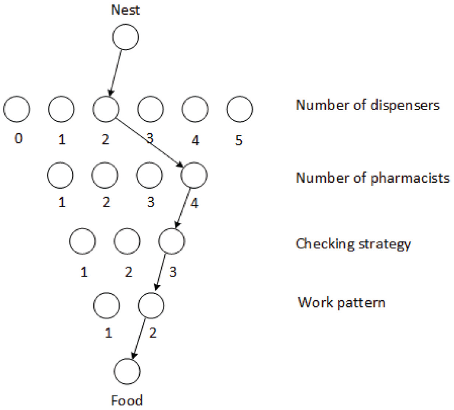
By assigning each of the decision variables a range of valid values, a state space for the optimisation problem can be constructed. Figure 4 shows a set of nodes representing the state space of the problem within the ACO framework. The state space is made up of layers of nodes, where arcs exist between the layers, but not within. Ants must choose a single node from each layer to create a route from their nest to the food source. For example, the path in Figure 5 corresponds to a pharmacy set up with two dispensers and four pharmacists, using checking strategy 3, and work pattern 2.

Figure 5.

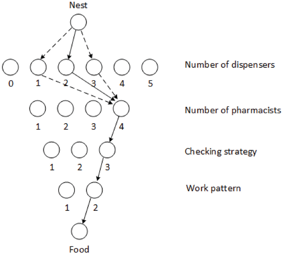
Local search implementation.

Note that there is a legal requirement for a pharmacist to be present if a pharmacy is going to dispense prescriptions. There is no such requirement for dispensers, that is a pharmacy can operate without dispensers. The maximum values of d and p have been chosen to be representative of a small to medium sized pharmacy in the UK. The three checking strategies are proposed:

1. A single check is performed by the pharmacist.

2. Two checks, the first done by a dispenser, and the second by the pharmacist. Any errors which are found are sent back to stage 2 to be dispensed again.

3. Two checks are performed as in 2. Any errors which are found by dispensers are attempted to be fixed straight away, without going back to stage 2. Pharmacists send errors to be dispensed again.

Each strategy is feasible, although precise prevalence of each strategy in day to day practice is unknown. During the data collection study, a mixture of checking strategy 2 and 3 were observed. Dispensers would regularly check their own prescriptions for accuracy in an informal way.

1. Pharmacists are able to contribute to primary dispensing tasks, such as receiving prescriptions from patients or dispensing prescriptions.

2. Pharmacists are unable to contribute to primary tasks.

There are 132 unique pharmacy set-ups in this problem ((6 × 4 × 3 × 2) − 12 = 132), since 12 set-ups are inappropriate because they have 0 dispensers and use work pattern 2 where pharmacists do not complete primary tasks. These set ups are not valid as there are no dispensers to complete primary tasks, and the pharmacists will not complete primary tasks when using work pattern 2, no primary tasks would ever be completed.

Cost of wages

The cost of employing the required staff for each set up is taken into consideration. According to the Office of National statistics, in 2015 the median earnings of UK pharmacists was £ 41,500, and £ 21,134 for a dispensing technician. ⁵⁵ Therefore, the cost of wages is calculated using equation (8):

$$\mathrm{Cost}=41,500\times \mathrm{p}+21,134\times \mathrm{d}$$

(8)

Local search

ACO algorithms can also make use of localised search patterns. This is a situation where the path of an ant which has returned a good solution is modified slightly, based on the belief that other good solutions may be in the surrounding neighbourhood. In this implementation of MMAS, a local search step is applied after the initial search phase. In the initial search a number of ants construct and evaluate solutions, of which the best ant is sent to a local search. The local search works as follows: one of the layers of nodes is randomly chosen for a local search with uniform probability. The path is kept constant except in the layer being locally searched, where the nodes 1 above and 1 below are tested. In the case of the work pattern, only the other option is tested. Figure 5 shows an example of how the local search is applied.

Heuristic information

One of the requirements of the optimisation is to find low cost solutions to the problem. To have the option of incorporating this preference, where a cost is associated with choosing an option, the cost using equation (9):

$${\nu }_{\mathrm{ij}}=\{\begin{array}{c}1/\left(j{C}_d\right)\mathrm{if}i=\mathrm{nest},\mathrm{j}\in L_1\hfill \\ \multicolumn{1}{c}{1/\left(j{D}_p\right),\mathrm{if}i\in L_1,\mathrm{j}\in L_2}\\ \multicolumn{1}{c}{1\mathrm{else}}\end{array}$$

(9)

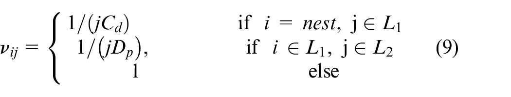
where ν_ij is the heuristic value for node j if an ant is on node i. L₁ and L₂ are the first and second layer of nodes in the search space, C_d is the cost of a dispenser, and C _p is the cost of a pharmacist in £1 × 10^4. For example, the heuristic value from the nest to a node indicating a solution with one dispenser, has a heuristic value of 1/2.1134 ≈ 0.48. The optimisation method used in this paper is a novel 3 stage approach. The optimisation will be run 3 times, where each iteration will use a different set of heuristics. The first stage will not use any heuristic information, the second stage will encourage the exploration of cheaper solutions, and the final stage will use an inverse cost heuristic to encourage the exploration of more expensive solutions.

Utility function

When evaluating the performance of each set up, there are multiple variables used to consider whether it was a successful set up. In this paper, the average waiting time, the number of errors, and the number of prescriptions completed are used. This represents a multi-objective optimisation problem. To transform this multi-objective optimisation problem into a single objective optimisation, a three termed utility function is proposed, shown in equation (10):

$$\mathrm{U}={\lambda }_1{\mathrm{X}}_{\mathrm{Waiting}}+{\lambda }_2{\mathrm{X}}_{\mathrm{Errors}}-{\lambda }_3{\mathrm{X}}_{\mathrm{Completed}}+\gamma$$

(10)

where λ₁, λ₂, λ₃ > 0. The terms in equation (10) are defined as follows, X_Waiting is the average time taken to dispense prescriptions, X_Errors is the number of errors dispensed to patients, and X_Completed is the average number of prescriptions completed. Better solutions to the problem will minimise the value of the utility function, U. Such solutions will, therefore, minimise the waiting time and the number of errors, while maximising the number of prescriptions being completed. A constant of γ = 30 is added to ensure positive value of all evaluations. Each of the variables were considered to be of relatively equal importance, so the three weighting variables were chosen such that the value of each of the variables would be of the same order. λ₁ was chosen to be 0.1, λ₂ was chosen to be 60, and λ₃ was chosen to be 0.1. These weightings imply that an improved average waiting time of 5 min, has the equivalent value of reducing the average number of errors by 0.5 per day, or completing 300 more prescriptions.

Pheromone update

In this paper the pheromone updates were controlled using a cycle of 3. Every third pheromone update was done by the best ant found so far, and every other update was done using the iteration best ant. Pheromone evaporation and secretion were implemented, as described in section 4.2.

Results

This Section presents the results of the optimisation. When applying the optimisation, checking the entire state space exhaustively can be avoided. The algorithm can generate optimal solutions using fewer simulations than would be required in an exhaustive search. The three optimisation stages combined used a total of 750,000 simulations. To test the Pareto optimal solutions generated by the ACO, an exhaustive search was also conducted on the state space. During the exhaustive search each possible pharmacy set up was simulated 15,000 times, which required 1980,000 simulations.

Algorithm implementation

The proposed MMAS optimisation algorithm used two ‘phases’ for each generation of ants crossing the state space. The first ‘phase’ used four ‘search’ ants, where each ant constructed a solution on the state space, and returned an objective value after simulating the CPN with a set-up corresponding to their path choice 500 times. The path of the ‘search’ ant which returned the lowest objective value, was then passed to the local search (the second phase). The local search tested the original path a further 500 times, and then checked each of the neighbouring variations another 1000 times each. Pheromone trails were updated at the end of each iteration, by applying pheromone to the path that returned the best objective value.

As proposed the MMAS algorithm was run in three ‘stages’. Stage 1 did not use any heuristic information, stage 2 included heuristic information which encouraged the exploration of cheaper solutions, and stage 3 used heuristic information which encouraged the exploration of more expensive solutions. Each optimisation ‘stage’ was run for a maximum of 50 iterations, with a stopping condition such that if the same iteration best path was returned 3 times consecutively the algorithm would terminate. The Pareto optimal solutions were found for the results of each instance of the algorithm before being combined into a single set of solutions. The parameters used during each stage of the optimisation are shown in Table 4.

Table 4.

MMAS parameter settings.

Parameters	1	2	3
α	1	1	1
β	0	1	1
ρ	0.98	0.98	0.98
${\nu }_{\mathrm{ij}}$	n/a	$\{\begin{array}{c}\frac{1}{C}\mathrm{if}C>0\hfill \\ \multicolumn{1}{c}{1,\mathrm{if}C=0}\end{array}$	$\{\begin{array}{c}\frac{1}{C_{\max }-C}\mathrm{if}C\ne C_{\max }\hfill \\ \multicolumn{1}{c}{1\mathrm{if}C=C_{\max }}\end{array}$
m	4	4	4
τ_0	48.2	48.2	48.2

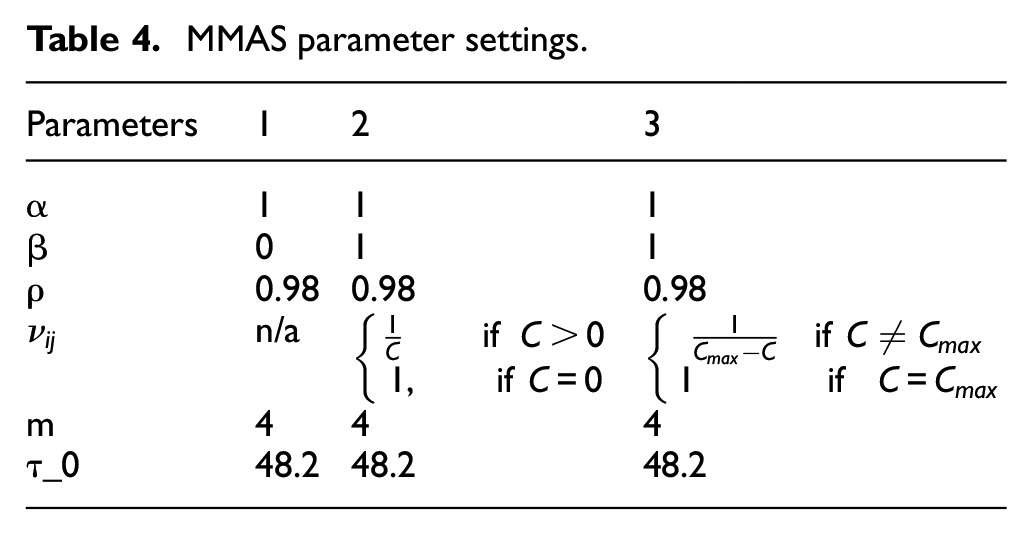
The evaporation rate, ρ = 0.98, has been used previously in Stützle and Hoos ²⁰ and Zecchin et al. ³⁷ it is common for ρ to be between 0.95 and 0.99. ⁵⁴ The size of the ant colony was set to be 4, this is at the lower end of potential colony sizes, ⁵⁶ since the optimisation state space is relatively small. A β value of 0 is used during the first stage since no heuristic data is used, and the following stages use a β value of 1 so that the different heuristics are taken into account.

Combining and comparing results with the exhaustive search

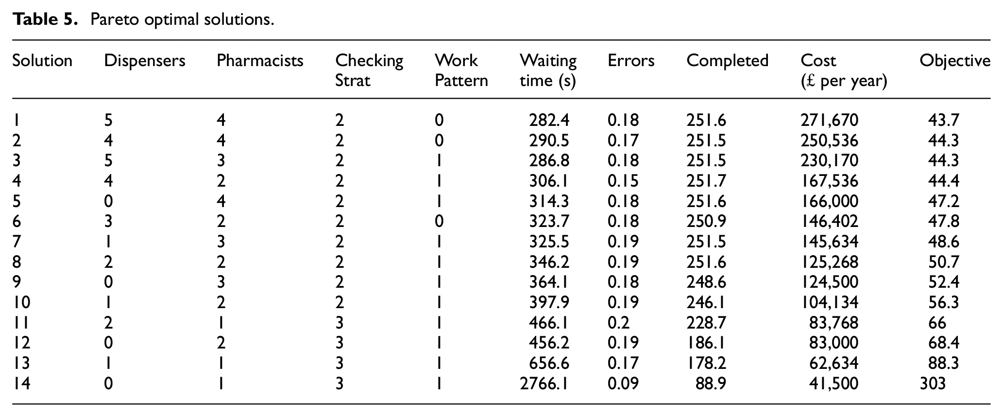
Overall, the MMAS optimisation evaluated 84 unique solutions at the local search level. The combined results from all three stages are plotted in Figure 6. Of the 84 solutions, 14 set-ups were non dominated, that is each solution in this set, cannot be improved without increasing the price, shown in Table 5. The optimal set up, was a team of five dispensers and four pharmacists, using a combination of checking strategy 2, and a non-flexible work pattern. Each stage of the optimisation contributed at least one Pareto optimal solution that was not found by the other stages. Stage 1 contributed four unique Pareto solutions, stage 2 contributed two unique Pareto solutions, and stage 3 found only a single unique Pareto solution. All other solutions were found by multiple stages.

Table 5.

Pareto optimal solutions.

Solution	Dispensers	Pharmacists	Checking Strat	Work Pattern	Waiting time (s)	Errors	Completed	Cost (£ per year)	Objective
1	5	4	2	0	282.4	0.18	251.6	271,670	43.7
2	4	4	2	0	290.5	0.17	251.5	250,536	44.3
3	5	3	2	1	286.8	0.18	251.5	230,170	44.3
4	4	2	2	1	306.1	0.15	251.7	167,536	44.4
5	0	4	2	1	314.3	0.18	251.6	166,000	47.2
6	3	2	2	0	323.7	0.18	250.9	146,402	47.8
7	1	3	2	1	325.5	0.19	251.5	145,634	48.6
8	2	2	2	1	346.2	0.19	251.6	125,268	50.7
9	0	3	2	1	364.1	0.18	248.6	124,500	52.4
10	1	2	2	1	397.9	0.19	246.1	104,134	56.3
11	2	1	3	1	466.1	0.2	228.7	83,768	66
12	0	2	3	1	456.2	0.19	186.1	83,000	68.4
13	1	1	3	1	656.6	0.17	178.2	62,634	88.3
14	0	1	3	1	2766.1	0.09	88.9	41,500	303

Figure 6.

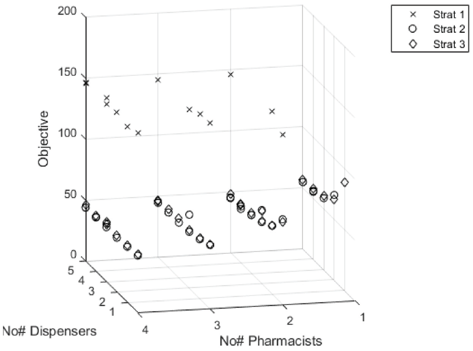
Objective state space for combined stages 1–3.

Table 5 shows the set of Pareto optimal solutions for the problem. The solutions in the Pareto front were made up of teams containing either a majority of dispensers (5), a majority of pharmacists (6), or an equal number of each (3). Solutions from 1 to 4 were high quality solutions, performing almost as well as the optimal set up.

The solutions from 5 to 14, were of increasingly worse quality, with solution 14 being significantly worse than the rest. A general trend is: if money is not limited, better teams will be those with a high number of staff, with either an equal number of each staff type, or more dispensers. However, if the budget for hiring staff is limited, the best set-up may contain fewer staff, and it’s likely that the best set-up will contain a majority of pharmacists.

A Pareto set of solutions was developed for the results of the exhaustive search. Solutions from 7 to 14 returned by the ACO algorithm appeared in exactly the same order and position as in the set of Pareto solutions generated by the exhaustive search. Solutions from 1 to 6 from the ACO algorithm did not appear in the exhaustive search Pareto front, although four solutions were very close, that is solutions 1, 3, 4 and 6 all appeared in the exhaustive Pareto front, but using the alternative work pattern.

It was noted when looking at the results of the exhaustive search that many solutions using the same staff set up and checking strategy would return similar objective values. Only solutions 2 and 5 from Table 5 made no appearance in the exhaustive Pareto front. These may have been considered optimal by the ants due to a lack of familiarity. For example, after a close look at the results it is clear that solution 5 was tested only once (1000 simulations) by the ants throughout all three stages of the optimisation, and the strong evaluation of this solution may be due to a small variation due to the randomness inherent in CPN simulations. On the other hand, in some cases, the preference of the ants for alternative work patterns with the same set ups may be justified. The ants evaluated solution 1 in Table 5 to be preferable to the same set-up with a flexible work pattern (the best solution from the exhaustive search), and during the optimisation both variations were tested 27 times (27,000 simulations). Hence the ants indicating that this set-up is preferable in this instance should be considered more valid than the result of the exhaustive search since they have simulated both solutions more times. In summary, the optimisation results compare well to the results generated by the exhaustive search, although results that the ants consider optimal that have only been tested a small number of times should be verified by further simulations before being put into practice.

The Pareto front is only a small subsection of the results generated during the optimisation. If a decision maker were to specify a price, it would be possible to provide a large variety of non-Pareto optimal solutions at that price point. The set ups would not be optimal, however having a set of options to choose from would allow for alternative configurations when there are staff or resource shortages.

Conclusion

In conclusion, this paper has shown that Max-Min Ant System is a viable algorithm for optimising a community pharmacy Coloured Petri Net simulation model. Furthermore, the CPN model has shown to be a suitable way to describe community pharmacy dispensing processes. The rules of the ACO algorithm have been presented, along with an explanation of how to apply the algorithm to a community pharmacy problem. Quantitative data collected from two UK pharmacies has been reported and incorporated into the CPN. A novel three stage heuristic inversion search was proposed and implemented in the MMAS algorithm. The cost heuristic inversion method was useful for identifying novel strong solutions, as every stage of the algorithm contributed at least one solution to the combined Pareto front, that were not found in any other stage. This model would be able to support pharmacy decision makers to choose the lowest cost pharmacy set ups that meet specific safety and efficiency requirements.

The paper aims to lay a blueprint for how more targetted simulation work would aid decision makers when choosing how to run community pharmacies. An issue to be aware of when modelling pharmacies, is that no two community pharmacies are exactly alike. Thus findings from this set of simulations may not apply to all pharmacies. It is suggested that more targetted modelling would be the way to best inform actual on the ground policy changes within pharmacies. In larger chain pharmacies, many of their stores are of a similar nature, using similar work patterns. It is possible that a more targetted model focusing on modelling a pharmacy from a larger chain would be able to support decision making about staffing levels, work patterns, and checking strategies.

The paper has shown that a pharmacy can be simulated and optimised using a CPN model and an ACO algorithm. Here we have modelled a generic pharmacy which is an amalgam of the four sites visited during data collection. To provide actionable decisions, the modelling should be tailored to a specific pharmacy. This could include measuring how many prescriptions they process throughout the day, how many of them are walk-ins versus delivery prescriptions, and recording how many of each of the advanced pharmacy services they complete. If the CPN were tailored to very accurately match the working processes of one specific pharmacy, the results produced by the optimisation would be more appropriate for decision makers to consider.

Comparing the results produced by the exhaustive search with those produced by the ACO algorithm showed that the ACO algorithm found the majority of the best solutions available to the problem. In total, 9 of the setups found to be Pareto optimal by the ACO, were also in the Pareto front of the exhaustive search. Solutions 1–4, and solution 6 were not in the Pareto front of the exhaustive search. The ACO algorithm was not so effective at distinguishing between solutions that have very similar objective values. In particular, it seems that set-ups containing large numbers of staff would produce very similar objective values when using the alternative work patterns. Using the ACO algorithm was more computationally efficient than testing the state space exhaustively (750,000 simulations vs 1,980,000). Future work could look at how best to choose the optimisation parameters, investigate the convergence rate of the algorithm, and as some data samples in this study are small, further data could be collected to obtain larger samples.

In addition to the above technical contributions in this area of work, this study also demonstrated how some reliability modelling and assessment methods, which are commonly used in modelling industrial systems, can be successfully applied in the area of healthcare systems, when the reliability and efficiency of their procedures are of paramount importance to society. Future studies could explore the potential of such techniques in other more complex healthcare settings, where procedures are carried out by clinical teams.

Future work could also include extending the state space of the optimisation problem. This could be achieved by either including more variables in the set-up configurations, or by increasing the current range of values. Two candidate variables to include in an extended optimisation are: the number of labelling stations available, and which tasks should be given priority when staff are working.

The work could be further extended by considering how to best set-up multiple pharmacies. Additionally, data collection on different types of staff perform tasks could be easily incorporated into the model. Investigation into the efficacy of different types of accuracy check, comparing ACT’s with pharmacists for example, could allow for a more effective optimisation between cost and safety.