Sage Journals: Discover world-class research

Abstract

This article presents a case study determining the optimal preventive maintenance policy for a light rail rolling stock system in terms of reliability, availability, and maintenance costs. The maintenance policy defines one of the three predefined preventive maintenance actions at fixed time-based intervals for each of the subsystems of the braking system. Based on work, maintenance, and failure data, we model the reliability degradation of the system and its subsystems under the current maintenance policy by a Weibull distribution. We then analytically determine the relation between reliability, availability, and maintenance costs. We validate the model against recorded reliability and availability and get further insights by a dedicated sensitivity analysis. The model is then used in a sequential optimization framework determining preventive maintenance intervals to improve on the key performance indicators. We show the potential of data-driven modelling to determine optimal maintenance policy: same system availability and reliability can be achieved with 30% maintenance cost reduction, by prolonging the intervals and re-grouping maintenance actions.

Keywords

Maintenance modelling failure modelling reliability availability rolling stock

Introduction

Public transportation networks are being consistently indicated as a key player to ensure sustainable, affordable, and high-quality mobility in urban areas.¹ In reality, much has still to be done to ensure a high level of system performance when providing safe and comfortable transport services to its customers. High level of system performance comes from carefully planned operations and a high availability of the asset during operations (reliability of operations, disturbances, and disruptions) as well as outside operations (workforce for maintenance and repairs, availability of extra vehicles to run the planned services). Keeping a high level of service encompasses these three aspects which are conflicting, with direct impact on capital-intensive issues.²

This article presents a case study to support decisions by a public transport operator, Haagsche Tramweg Maatschappij (HTM), which manages and operates tram and light rail systems in the region of The Hague, The Netherlands. The main decision to be tackled is to balance maintenance operations (cost and workforce required) versus system performance, expressed in terms of reliability and availability. The maintenance actions of HTM follow a pre-determined maintenance policy: a set of preventive maintenance (PM) tasks is performed at fixed, distance- or time-based intervals. The maintenance policy is the sequence of tasks with a positive impact on the performance and life expectancy of the subsystem and its components, described in terms of task level (ranging from a simple check to a full repair), and their timing.

We focus on the braking system of light rail rolling stock (Alstom Citadis), more details in Appendix 1. For light rail rolling stock, it is currently the task of the manufacturer to determine a maintenance policy on forehand, based on reliability, availability, maintainability, and safety (RAMS) specifications and based on the degradation, failures, and repairs expected in the warranty period. Maintenance tasks and intervals were never evaluated, and it is suspected (based on experience and gut feelings, not on quantitative indicators) that they are very conservative, resulting in a high workshop load and high maintenance costs. The goal of this article is to report on a test case on dedicated optimization of PM policy which targets directly reliability, availability, and maintenance costs. We combine the existing failure records with a dedicated maintenance model to improve the maintenance of a rolling stock system.

The main contribution of this article is the application to a relevant test case of a comprehensive approach used to determine a PM policy and comparison against the current state of practice. To the best of our knowledge, no similar test case bridging data-driven failure modelling and data-driven maintenance modelling has been reported yet in the literature, despite its very high practical interest. The approach proposed goes through the following systematic steps:

Failure modelling: describing the failure behaviour with Weibull functions. The values of Weibull coefficients were also derived from the recorded failures.

Characterization of maintenance actions and related costs: the downtime and costs of preventive and corrective maintenance actions are determined based on recorded data.

Development of the maintenance model: the model relates the maintenance actions with the failure behaviour, based on the sequence of PM actions, and time intervals between them. We consider three levels of PM actions, based on Tsai et al.³

Model validation and sensitivity: we determine the sensitivity, influence of uncertainties, impact of input parameters, and uncertainties related to model’s input parameters towards availability and costs. A benchmark maintenance model is determined for the current maintenance policy and validated against observed availability and costs.

Definition of optimal maintenance policy for a given key performance indicator: the model is used to determine maintenance policies aimed at the maximum reliability, maximum availability, and minimum costs, and a compromise between them.

Based on available historical data of past repairs and maintenance actions, optimized maintenance policies can be determined, which allow consistent savings compared to current approaches, while keeping the operational performance higher than current state of practice. We schematize the combination of data-driven system modelling, expert knowledge, and company strategies and objectives in Figure 1. We remark that due to the confidentiality of the data, we can only report aggregated and relative improvements, concerning the company objectives.

Figure 1.

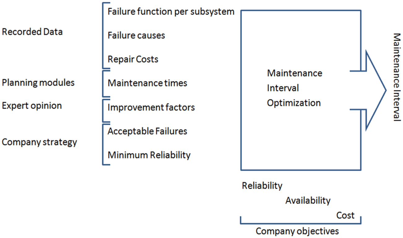
Combination of approaches identified to determine the optimal maintenance policy.

The article is organized as follows. Section ‘Literature review on PM’ reports on the existing literature. Section ‘Modelling failure functions’ describes the possibilities given by data-driven approaches for modelling failures and definition of maintenance actions. Section ‘Modelling PM’ determines the maintenance model, and proposes an optimization scheme targeting a set of key performance indicators, which is evaluated in section ‘Results and discussion’. Section ‘Conclusion and recommendations’ concludes the research, with directions for future research. This article is based on Kraijema.⁴

Literature review on PM

Applications of PM to rolling stock systems have often analysed and targeted a single subsystem rather than a holistic perspective of the overall system (air conditioning system⁵ and door systems⁶). We also point to the reader to Giacco⁷ for a longer discussion of maintenance issues in rolling stock. In general, PM targets avoiding the system failure and keeps the system available and reliably working for longer periods. In fact, PM actions are proactive in nature and are performed before the systems fail. There are various models of the effects of PM actions on the overall performance of the system; this section gives a short overview of the possible models. For systems where a condition based monitoring system cannot be easily set up, most research efforts are currently directed to better quantifying the intervals for PM and modelling the impact of different maintenance levels and maintenance operations. We call this a PM policy: the set of maintenance actions that are to be performed on specific components or subsystems of a technical system. It also defines the maintenance intervals for these actions.^8,9

There are three types of models that can be used to describe the relation between the failure behaviour of a system and components (SC) and the applied maintenance policy:

Constant failure rate (age reduction PM): the failure rate, as a function of the effective SC age, is assumed the same throughout its life cycle. The effects of PM actions are modelled by an effective age reduction (for the period of PM action τ > 0) of the SC, and the failure rate λ(t) becomes λ(t − τ).

Failure rate reduction: the second category assumes that the effects of PM actions on the SC’s failure behaviour are modelled by a reduction of the failure rate of the SC, that is, the failure rate λ(t) becomes $a \cdot λ (t)$ , where $a \in (0; 1)$ .

Combined: the effect of PM actions is modelled by a reduction of the effective system age as well as the failure rate, that is, the failure rate λ(t) becomes $a \cdot λ (t - τ)$ for linear models or $λ (c \cdot t + d)$ for nonlinear models.

All these modelling approaches use the failure distribution function to predict the SC’s reliability. The distinctive difference is found in the way the assumed failure behaviour continues after PM actions are performed. PM actions influence the failure times of system and components (SC). PM actions are described in literature in three typical classifications: perfect, minimal, and imperfect.¹⁰ Perfect PM actions restore the system to an optimal state, that is, the reliability of the system is increased to the ‘As Good As New’ (AGAN) level. Minimal PM actions restore the system to a state comparable to the state just before the maintenance actions were performed, that is, the reliability is increased by a minimal amount. This is referred to as ‘As Bad As Old’ (ABAO). Most PM actions performed in real life are neither perfect nor minimal. These in-between actions are often referred to as imperfect PM. In general, imperfect maintenance models can be grouped into following groups: age reduction models,¹¹ hazard rate reduction models,¹² combined age-hazard reduction models,¹³ and others.¹⁴ Detailed overview of different PM policies can be found in Pham and Wang¹⁵ and Wang.¹⁶

Cheng et al.¹⁷ proposed a linear PM model that optimizes the PM intervals between preventive replacements by minimizing the cost while maintaining a certain minimum level of reliability. The systems reliability is derived from a Weibull failure rate distribution. An improvement factor µ is introduced to model the effects of PM actions on the system’s effective age. This means considering a = (1 − µ) and b = 0. Schutz and Rezg¹⁸ proposed a nonlinear PM model based on the effectiveness of PM actions on the system reliability versus cost. The effectiveness factor ρ and PM interval length T define the effective age reduction of the system. This means considering c = (1 − ρ) and d = T. Cheng and Tsao¹⁹ stated that PM actions do not always directly reduce the systems effective age or failure rate. PM actions such as cleaning, adjusting, or lubricating will only impact the systems degradation rate and will not improve the reliability of the system.

Coria et al.²⁰ proposed a maintenance model with a more general relation between PM interval and failure rate. Weibull parameters can thus be estimated from real-life failure time data of a system that has been maintained from day one. Imperfect PM actions are performed at fixed intervals t_k = kT, with T length of the PM interval. Tsai et al.³ also use three different levels of PM actions. This provides the ability to closely match the real-life situation and allows for detailed insight into cost savings at a higher system availability and reliability level than models that only consider component replacement. The improvement of PM actions to the reliability is described as a function of the failure mechanisms of the component. Based on the literature surveyed, we found that the models of Coria and Tsai were the most suitable for the rolling stock system due to the possibility to leverage imperfect data about past (possibly imperfect) maintenance tasks.

Modelling failure functions

Available data of recorded failures and identification of subsystem

We start from a database of about 2200 failure, repairs, and maintenance actions which span 5 years between 1 January 2010 and 31 December 2014. In this period, a uniform maintenance policy has been used, for the entire fleet of light rail rolling stock. Burn-in of the vehicles is neglected as the vehicles started operations in 2006. Instead, a period of 2 weeks (estimated with the help of the maintenance engineer (HTM, personal communications, 2015)) is considered after each maintenance action to avoid considering burn-in or imperfect repairs. We filtered the dataset as to not consider censorship, by restricting to a set of records where maintenance actions were anyway performed at fixed intervals, and have been numerous, for all vehicles considered. Relaxing this assumption only needs different methods for estimation of failure rate.²¹

Among the subsystems, the braking system has been selected as the most relevant one, being responsible for more than a third of failures, costs, and downtime (see Appendix 1). This has a direct impact on the maintenance policy of the rolling stock systems. The braking system is functionally divided into the four following subsystems: brake control, hydraulics, magnetic track, and electro-dynamic (ED) braking. This latter is excluded from the study as no failure has ever been recorded.

Failure data for the remaining three subsystems are available from different sources: vehicle diagnostics system, driver input, work from inspection, and work order data. Each of these data sources were used and crosschecked to get detailed failure records. The information provided on the corrective work orders will be used to derive the distance to failures for each of the components in the braking system. The mean distance between failures (MDBF) of components in the braking system (the equivalent for transport units of the mean time between failures (MTBF), with the distance covered replacing the time elapsed) can be derived more accurately based on the position of the failed component. When this data are not reported in the computerized maintenance management system (CMMS), information might be given by the mechanic as a remark on the repair work order.

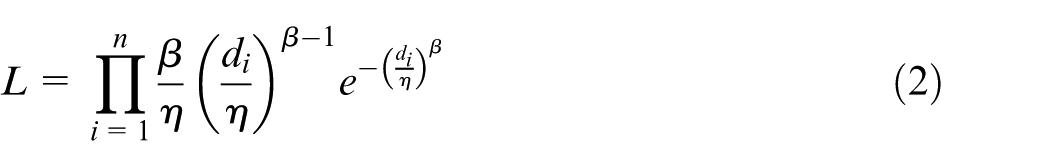
For each of the subsystems, a standard Weibull distribution was used to characterize the failure rate; the scale and shape factors of Weibull distributions are determined from recorded failures to model their failure behaviour. Due to the fact that most failure repairs are imperfect or not effective at all, those distributions cannot be fitted right away.

Failure rate modelling

The failure rate distribution is modelled by means of Weibull distribution, where travelled distance was used instead of time.²² The distance between failures of the components in the braking system is also influenced by the current PM policy. Formally, the failure probability density function is defined as

f (d) = \frac{β}{η} {(\frac{d}{η})}^{β - 1} e^{- {(\frac{d}{η})}^{β}}

(1)

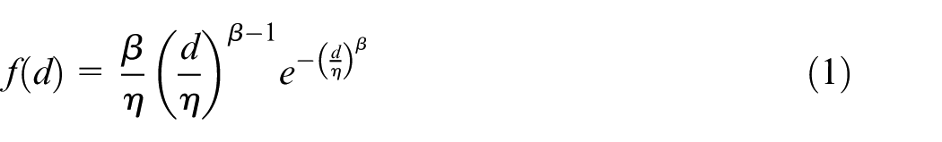
where f is the failure probability distribution function, d is the distance travelled between failures, $β$ is the shape factor of Weibull distribution, and η is the scale factor of Weibull distribution. Weibull parameters are generally estimated using graphical^19,23 or analytical fitting methods.^20,23,24 Based on the experiments proposed in Coria et al.,²⁰ we used a common maximum likelihood estimation (MLE) procedure to determine the Weibull parameters of the system under the current PM policy, where d₁, d₂, …, d_n are actual distances to failure from the data

L = Π_{i = 1}^{n} \frac{β}{η} {(\frac{d_{i}}{η})}^{β - 1} e^{- {(\frac{d_{i}}{η})}^{β}}

(2)

The data give sufficient evidence that the failure rates of three subsystems are almost constant.

Reliability related to maintenance actions

Three PM actions considered in this model are:

Service (PM1): this includes easily performed maintenance actions such as cleaning, adjustment, retightening, refilling, or adding consumables (oil, grease, etc.). Service actions are assumed to help maintain the SC’s current state of reliability. The current level of reliability is not improved, but the rate of deterioration is reduced.

Low-level repair (PM2): this includes more time-consuming PM actions, such as small spare part replacement in addition to the service activities. Low-level repair is assumed to improve the SC’s reliability to a state in between AGAN and ABAO.

High-level repair (PM3): this includes SC overhaul or replacement. High-level repair is assumed to return the reliability to an AGAN state.

The effects that these PM actions have on the reliability of the SC are defined by two improvement factors m₁ and m₂. m₁ is used to alter the deterioration rate of the SC’s reliability after PM1, and m₂ is used to define the reliability increase after PM2. Using standard Weibull distributions for the failure rate, the reliability of the system after maintenance interval j with interval duration T is defined as

R_{j} (t) = R_{0, j} \cdot e^{- {(\frac{\frac{1}{m_{1}} (t - (j - 1) T)}{η})}^{β}}

(3)

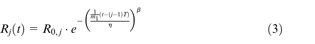
with

R_{0, j} = R_{f, j - 1} + m_{2} (R_{0} - R_{f, j - 1})

(4)

where R_0,j is the initial reliability at maintenance stage j, R₀ is the initial reliability of a new SC, and R_f,_j − 1 is the final reliability before maintenance in the previous stage.

The improvement factors can be defined as a function of some s failure mechanisms, for example, fatigue; wear (contact stress); ageing; and others, such as contamination, corrosion, and heat.²⁵ The improvement factors are defined as

m_{1 / 2} = \sum_{i} p_{f, i} \cdot I_{i}

(5)

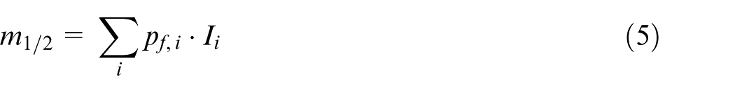
where i refers to the failure mechanisms, p_f is the failure probability, and I is the probability for system improvement caused by the PM action. The two improvement factor parameters m₁ and m₂ have value of 1 for high-level repair (PM3), m₂ has value of 0 for the service (PM1); in the other cases, they have a value between 0 and 1. Determining the precise value for those two parameters is a crucial task as it describes the influence of all maintenance actions. To this end, we refer to expert opinion.

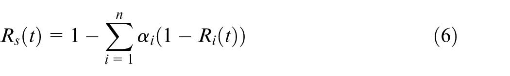
Tsai et al.³ optimize the system for availability, which also involves determining the relation between reliability and the maintenance actions performed. We here briefly introduce the key relations between those three concepts. The system-level reliability is defined using the Advisory Group on the Reliability of Electronic Equipment (AGREE) method,^26,27 assuming that the general system can be decomposed into a series of independent SCs, in this case the four braking subsystems. This leads to the expression of the reliability of the system over time, where α_i is the probability of system failure due to subsystem i

R_{s} (t) = 1 - \sum_{i = 1}^{n} α_{i} (1 - R_{i} (t))

(6)

The system-level availability in stage j is defined as

A_{s, j} = \frac{MU T_{s, j}}{MU T_{s, j} + MD T_{s, j}}

(7)

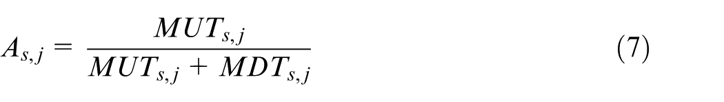
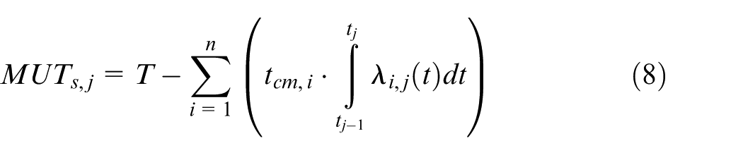
where MUT is the mean uptime of the system defined as

MU T_{s, j} = T - \sum_{i = 1}^{n} (t_{cm, i} \cdot \int_{t_{j - 1}}^{t_{j}} λ_{i, j} (t) dt)

(8)

And MDT is the mean downtime of the system defined as

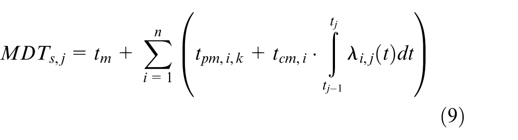
MD T_{s, j} = t_{m} + \sum_{i = 1}^{n} (t_{pm, i, k} + t_{cm, i} \cdot \int_{t_{j - 1}}^{t_{j}} λ_{i, j} (t) dt)

(9)

where t_cm,i represents the average repair time for subsystem i, t_pm,i,k is the time required to perform PM action k on subsystem i, and t_m is an additional system-level time for grouped maintenance actions. The average repair time t_cm,i is dependent upon the severity of the failure. All times are derived from the planning module of HTM. Braking system failures are always ‘critical’ for safety and need to be dealt with as soon as possible. This takes an extra downtime t_dt due to failure and includes the time required to evacuate passengers (if applicable), transfer of the vehicle to the depot, and waiting time for repair; t_cm,i,m is the mean repair time for subsystem i

t_{cm, i} = t_{m} + t_{dt} + t_{cm, i, m}

(10)

Modelling PM

Input parameters

The impact of maintenance actions on the failure behaviour is described by multiplying the failure probability with the improvement probability associated with the associated PM action per failure mechanism. We use the available failure records to estimate the failure probabilities per failure mechanism. The improvement probabilities of associated PM actions are instead estimated using expert opinion. However, before estimating the improvement probabilities of PM actions, it is necessary to define the content of PM actions. Table 1 gives an overview of the maintenance tasks that are assumed to be performed when a PM action is applied to the subsystem, and Table 2 gives an overview of the related parameters to each subsystems and failure cause.

Table 1.

Identification of subsystems and related PM actions.

Subsystem		PM action k
ID	Description	PM1	PM2	PM3
1	Brake control system	Clean Visual inspection Tighten loose connections Function check	Clean thoroughly In-depth visual inspection Function check Replace if necessary	Overhaul
2	Hydraulic brake system	Clean and lubricate Visual inspection Tighten loose connections Fill fluid if necessary	Clean thoroughly In-depth visual inspection Replace if necessary	Overhaul
3	Magnetic track brake	Clean Visual inspection Tighten loose connections	Clean thoroughly In-depth visual inspection Replace if necessary	Overhaul

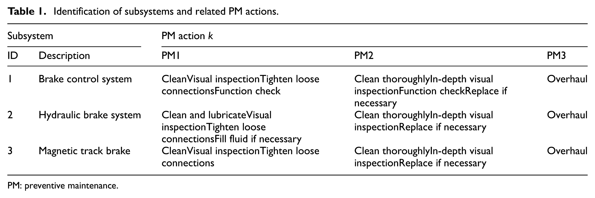
PM: preventive maintenance.

Table 2.

Parameter values for subsystems, PM actions, and failure probabilities (FP).

Subsystem	Parameter	Failures causes
1. Brake control system		Software	Ageing	Wear
	PM1: I_i	0.9	0.8	0.8
	PM2: d_i	0.9	0.9	0.9
	FP: p_f,i	0.6	0.2	0.2
2. Hydraulic brake system		Wear	Ageing	External	Fatigue
	PM1: I_i	0.8	0.8	0.8	0.5
	PM2: d_i	0.9	0.9	0.9	0.8
	FP: p_f,i	0.5	0.3	0.1	0.1
3. Magnetic track brake		Ageing	External	Wear
	PM1: I_i	0.8	0.8	0.8
	PM2: d_i	0.9	0.9	0.9
	FP: p_f,i	0.5	0.3	0.2

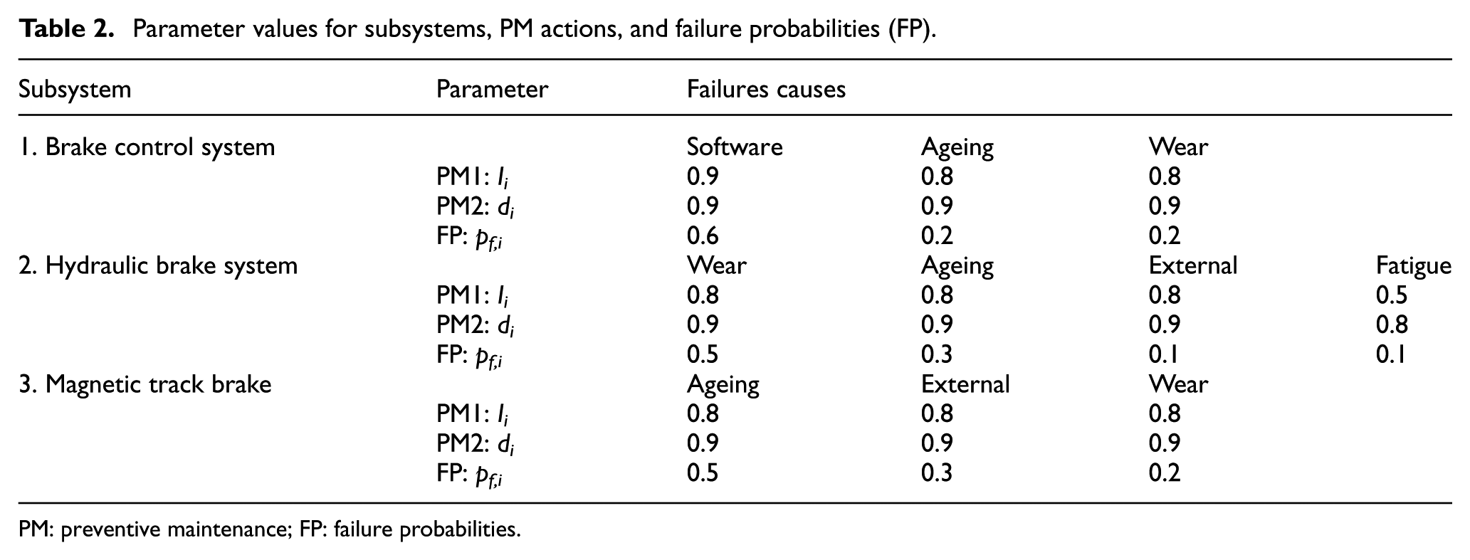
PM: preventive maintenance; FP: failure probabilities.

For each subsystem, we identified up to four common failure causes, which make up the majority of the failures and give the results of the failure cause analysis. We report in Table 2 the failure probability (as recorded in the CMMS) per cause and subsystem, and the estimated improvement factors associated with the PM actions, determined with help of maintenance experts from HTM. Here, m₁ can be computed as the improvement I_i to the operational condition of each subsystem, due to PM1 actions; m₂ is defined as the repair success rate d_i of PM2 actions.

PM model

We can finally determine the link between maintenance intervals and performance indicators: total costs, availability, and reliability. The total cost at system level, due to maintenance actions C_s,j in the jth PM interval depends on the sum of PM cost C_pm and Corrective maintenance (CM) cost C_cm

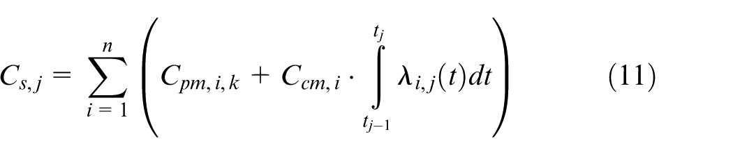
C_{s, j} = \sum_{i = 1}^{n} (C_{pm, i, k} + C_{cm, i} \cdot \int_{t_{j - 1}}^{t_{j}} λ_{i, j} (t) dt)

(11)

The components of equation (11) that are related to costs are defined using the CMMS system by deriving the internal hourly rates and spare parts costs.

Based on the expression of reliability in equations (8), (10), and (11), and the structure of the SC, different intervals t_p,I are associated to different subsystems, as they have independent, unrelated failure rate. For each subsystem, the smallest optimal subsystem-level interval t_p,i, based on maximizing the availability y, is:

(t_{p} + t_{pm}) λ (t_{p}) - \int_{0}^{t_{p}} λ (t) dt = \frac{t_{pm}}{t_{cm}}

(12)

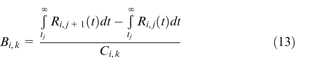
The optimal interval T which allows to keep availability always above the threshold can then be assumed to be the smallest of them, that is, T = t_p = min_i {t_p,I} Subsystems i with t_p,i = T receive maintenance at any maintenance interval; those with t_p,i > T receive maintenance when the reliability would decrease below the minimum acceptable reliability R_min within a time interval T, that is, before the next planned maintenance action. At any maintenance interval, the type of PM actions will be selected by means of a maintenance benefit function B_i,k. For the jth PM interval, benefit B_i,k is defined as the ratio between the reliability improvement and the cost involved

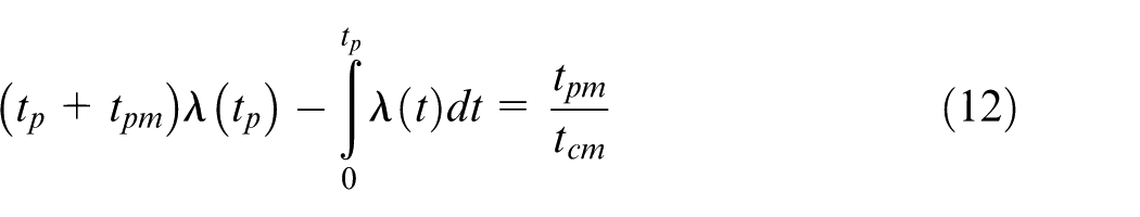
B_{i, k} = \frac{\int_{t_{j}}^{\infty} R_{i, j + 1} (t) dt - \int_{t_{j}}^{\infty} R_{i, j} (t) dt}{C_{i, k}}

(13)

The availability of the system can be expressed as in equation (7). To this end, we need to define the maintenance times associated with PM1, PM2, and PM3 and with the corrective maintenance actions. The mean downtime (MDT) due to PM, related to a given maintenance interval T, is defined as

MD T_{pm, s} = t_{m} + \sum_{i = 1}^{n} t_{pm, i, k}

(14)

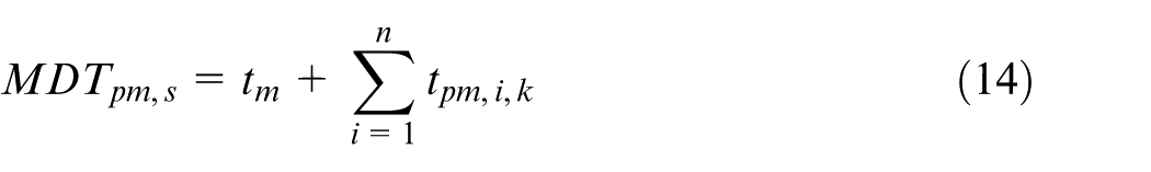
where t_m is the time required for the (overall) system-level maintenance, and t_pm,i,k is the time required to perform PM action k on subsystem i for all n subsystems.

The values of PM times t_pm,i,k and t_m in equation (14) are derived from the planning module in the CMMS system and verified by the maintenance engineer. The values of CM times (see equation (10)) are also derived from the CMMS system: t_cm,i,m mean repair time for subsystem i; t_dt, extra downtime due to failure of system I together with the extra downtime includes the time required to evacuate passengers (if applicable), transfer of the vehicle to the depot, and waiting time for repair.

Tsai et al.³ define the minimum reliability at the system level; while we define the minimum reliability at subsystem level and as a function of the risk associated with the failure of the subsystem. The risk of failure is calculated by relating the probability of occurrence with the impact on corporate objectives. Combining the calculated risk values with the minimum reliability, which is set by company policies to 0.85, the minimum reliability of each subsystem was calculated. The AGREE method is used, as presented in equation (7). The values of the system probability failure due to a specific subsystem can also be derived from CMMS: those are, respectively, 0.42, 0.44 and 0.14 for the brake control system, the hydraulic brake system, and the magnetic track brake.

Maintenance interval optimization

The optimization of the maintenance policy relates to choosing the interval of maintenance between maintenance stages j and the most beneficial maintenance action k for subsystem i in stage j. For maximizing overall availability, Tsai et al.³ determine analytically the minimum maintenance interval in the multi-component setting. The minimum interval drives the all maintenance process, based on some economic/structural dependence.²⁵ We remark that this approach is inapplicable in the system considered, as no explicit check of subsystem reliability is performed. Moreover, for the other performance indicators, a closed-form solution is not easy to derive. We thus resort on a simple sequential optimization approach to determine simultaneously maintenance interval and maintenance actions along time. The key problem investigated is the precise determination of the sequence of maintenance actions to be performed in a PM scheme, that is, when to perform which maintenance action, based on a set of performance indicators.

The algorithm is shown in Figure 2. The possible time intervals for maintenance (time_interval) are scanned in sequence within a range {min_time_interval; max_time_interval}. Given a time interval, the timing of PM maintenance is given. To determine the actions chosen, for all stages j until the expected end of life of the system, we determine the required and potential maintenance actions. The required maintenance actions are those that are required as the current reliability is below the threshold. Note that there is a substantial difference with the approach of Tsai et al.,³ where there is no minimum reliability setting prescribed. In the case when the most beneficial maintenance action k does not improve the reliability of the system to the minimum required level, the next best k is selected, which allows reaching the target reliability. The potential maintenance actions are those which would not be required at current stage j, but would be required between the current maintenance stage j and the next one j + 1. For those, the benefit function as in equation (13) is used.

Figure 2.

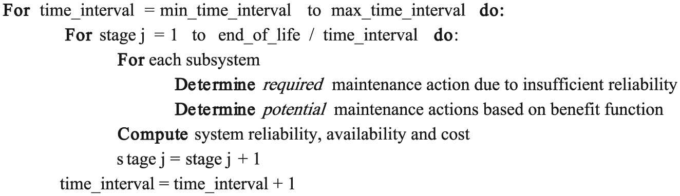
Pseudocode of the optimization approach.

The reliability, availability, and the costs are then assessed at system level. The time_interval which leads to the minimum costs, maximum availability, or maximum reliability is, respectively, selected. As final output of the optimization model, the sequence of maintenance actions is outputted, as well as the evolution of the performance indicators over time. The model is implemented in MATLAB R2014b and reports quickly the optimal maintenance interval, as well as the sequence of maintenance actions. Depending on the amount of intervals evaluated, the entire optimization takes between 5 and 45 min of computation time on a standard computer.

Model validation and sensitivity analysis

To validate the PM model of section ‘PM model’, a benchmark PM model was created by setting the system-level maintenance interval T to match the current maintenance policy together with all other input parameters. The resulting availability, PM cost, and CM cost compared favourably with the data extracted from the records (Table 3).

Table 3.

Relative difference in availability, PM cost, and CM cost between the calculated and recorded values.

Parameter	Description	Deviation from recorded value (%)
A_s	System availability	1.15
C_pm	PM cost	0.25
C_cm	CM cost	0.56

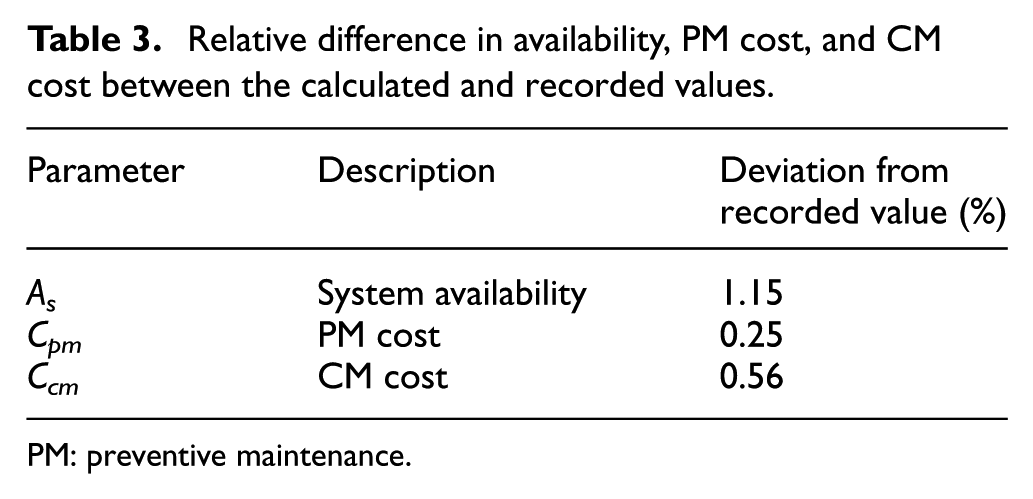
PM: preventive maintenance.

To determine the impact of changes, uncertainties, and error in estimation in the input parameters on the output of the model, we have performed a sensitivity analysis. Precisely, we evaluated the influence of the improvement factors (m₁ and m₂), maintenance times (t_pm and t_cm), maintenance costs (C_cm and C_pm), and minimum reliability (R_min) on the resulting availability and total maintenance costs. Table 4 gives an overview of the input parameters with their low and high values that are included in the sensitivity analysis. Both low and high values are selected in such a way that they represent the 90% confidence interval for the specific parameter. Note that the high values of parameters such as improvement factors and minimum reliability parameters are limited to a maximum value of 1.

Table 4.

Parameters and variations considered in the sensitivity analysis.

Parameter	Description	Low (%)	High (%)
m ₁	Improvement factors 1	−20	+20
m ₂	Improvement factors 2	−20	+20
t_pm	PM times	−20	+20
t_cm	CM times	−20	+20
C_pm	PM costs	−20	+20
C_cm	CM costs	−20	+20
R_min	Minimum reliabilities	−20	+20

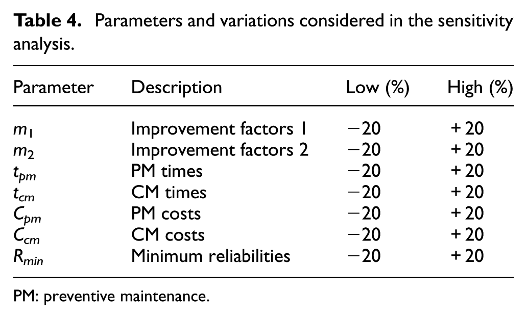
PM: preventive maintenance.

The sensitivity analyses for availability and total maintenance costs are reported as tornado charts in Figure 3. The reference value of output parameters is given by the vertical axis. The blue/red bars represent the output parameter value for the low/high input parameter values, respectively.

Figure 3.

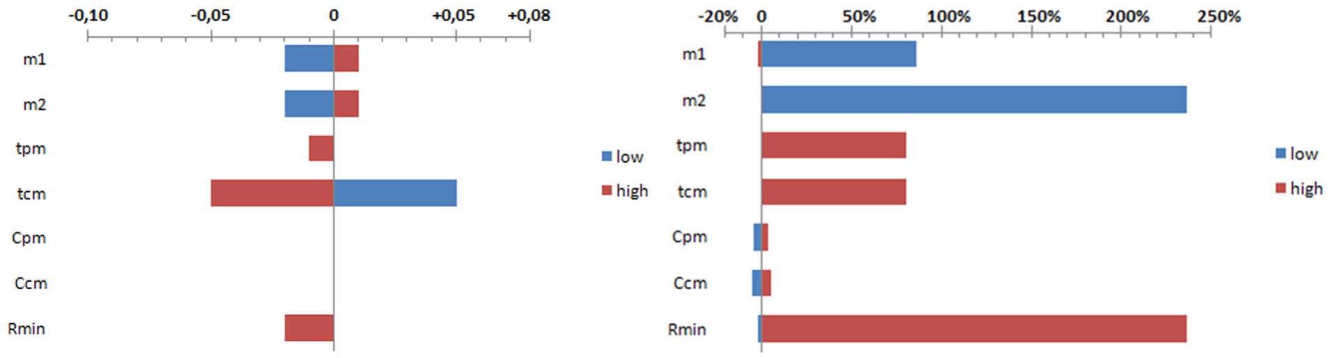
Model sensitivity: availability (left) and maintenance costs (right), in percentage of base case.

Looking at the results of sensitivity analysis for availability, it can be observed that t_cm has the highest influence on the availability. While this was not surprising, it was a surprise to see how strong the influence of improvement factors on the total costs is. If improvement factors were to be lower, then a higher level of PM actions is required to ensure the minimum reliability. An expert check on the interval derived confirmed the validity of the model.

Results and discussion

Results

We determine quantitatively the best maintenance intervals and their impact to the company objectives and the results correspond to the general intuition. Figure 4 shows how the maintenance interval has significant impact on the PM costs. The costs and intervals are reported scaled down to the benchmark policy currently implemented. Looking only at PM costs, the minimum is found for a maintenance interval which is about 90% longer. Even though a reduction of the maintenance interval significantly increases the reliability of the system, it also increases the PM cost (and reduces the availability, due to the continuous maintenance visits). This relationship is rather regular. A similar behaviour in cost increase is found, much stronger, for long maintenance intervals. After a certain threshold, PM costs jump significantly because high-level PM actions are required to recover the system to the desired reliability levels, and high-level PM actions yield higher maintenance costs. The erratic behaviour for very long maintenance intervals is due to the interaction of failures and the extensive repairs needed when maintenance is performed.

Figure 4.

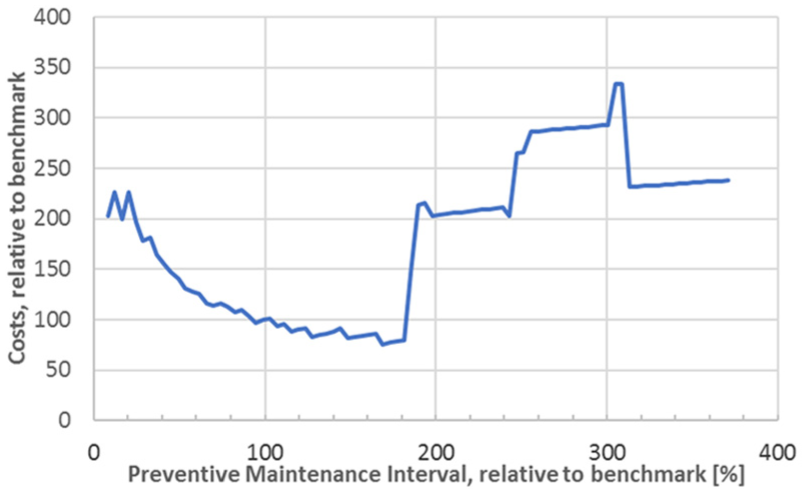
Total maintenance cost as a function of the maintenance interval, relative to the benchmark.

We now discuss the relationship between maintenance intervals and the performance indicators. Figure 5 shows the relation between maintenance intervals and reliability. The maintenance interval is reported relative to the benchmark, while the reliability is reported in absolute number. Two curves are plotted: the one reporting the mean reliability given a maintenance interval (R_s,mean, blue solid line) and the one reporting the minimum reliability given a maintenance interval (R_s,min, red dotted line).

Figure 5.

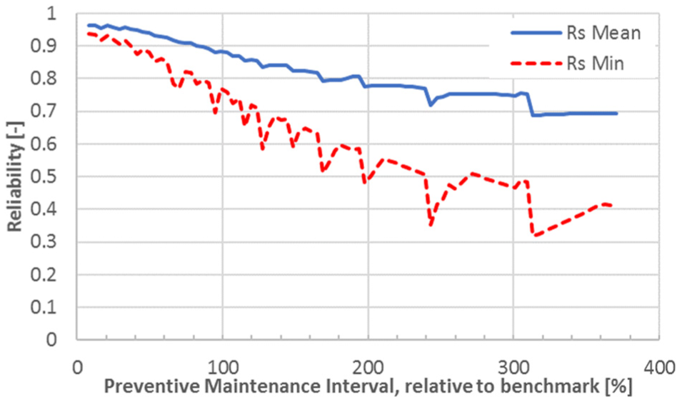
System-level reliability as a function of the maintenance interval.

It is evident from the figure how the R_s,min drops at a higher rate than the R_s,mean, since reliability before maintenance is directly decreasing with longer maintenance intervals, while the reliability after maintenance is roughly the same, after the PM actions are performed. Overall, high minimum reliability requirements are associated to a smaller maintenance interval, and therefore, increased maintenance cost of the system.

Figure 6 reports on direct connections between reliability, availability, and costs. Allowing the subsystem reliability to drop significantly below the minimum reliability R_min prescribed by the key performance indicators results in high PM cost. In this case, the only feasible PM action is PM3, which is the most expensive maintenance action. However, the maintenance cost rapidly increases when the minimum system reliability requirements exceed 0.85. The minimum costs, within the feasible range of intervals, correspond to a smaller reliability, as shown in Figure 6 (top). The resulting maintenance policy is very similar to the availability driven policy, in terms of maintenance interval. Figure 6 (bottom) shows the relation between minimum reliability and availability of the system. A rapid decrease in availability is observed when the minimum system reliability requirements exceed 0.85. This corresponds to increased system downtime due to short maintenance intervals. The availability of the current benchmark solution is the lowest, before the sharp increase in reliability. This is one of the motivations for choosing a different, optimized, maintenance interval.

Figure 6.

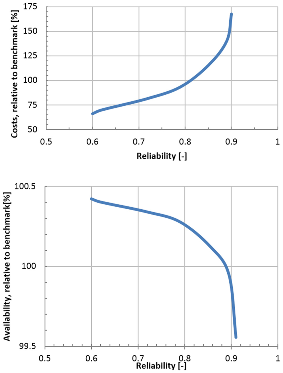
Relative maintenance cost (top) and relative availability (bottom) as a function of the minimum reliability for maintenance intervals between 30% and 180% of the benchmark interval.

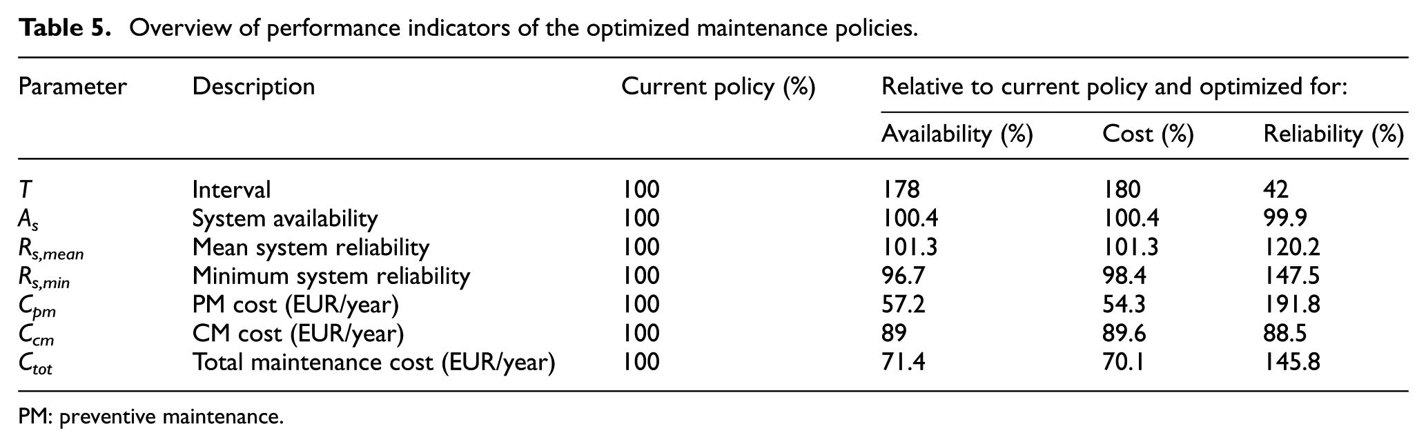
The results in the previous sections show that the total maintenance cost and system availability are highly dependent upon the minimum reliability requirements of the system. Both availability and cost driven maintenance policies allow the reliability of the system to drop below the accepted minimum. Table 5 gives the values of the key parameters for the availability-, cost-, and reliability-driven maintenance policies, relative to the current situation.

Table 5.

Overview of performance indicators of the optimized maintenance policies.

Parameter	Description	Current policy (%)	Relative to current policy and optimized for:
Parameter	Description	Current policy (%)	Availability (%)	Cost (%)	Reliability (%)
T	Interval	100	178	180	42
A_s	System availability	100	100.4	100.4	99.9
R_s,mean	Mean system reliability	100	101.3	101.3	120.2
R_s,min	Minimum system reliability	100	96.7	98.4	147.5
C_pm	PM cost (EUR/year)	100	57.2	54.3	191.8
C_cm	CM cost (EUR/year)	100	89	89.6	88.5
C_tot	Total maintenance cost (EUR/year)	100	71.4	70.1	145.8

PM: preventive maintenance.

Discussion

Compared with the benchmark figures of the current policy, both availability and cost driven maintenance policies show a potential maintenance cost reduction of 30%. They moreover maximize the system availability without sacrificing the current mean and minimum reliability; the maintenance intervals are almost 100% longer. The reliability-driven maintenance policy shows a potential increase of 20% in average system reliability and 48% of the minimum system reliability, without compromising the availability of the system or raising the total maintenance cost significantly. Increasing the reliability is related to achieve higher customer satisfaction. Interesting directions for integral assessment of maintenance in transport systems direct towards the level of service, by means of quantifying uncertain travel time and delay in operations²⁸ or in evaluating the societal costs of delay as perceived by the different users.

A key feature of the system is the strong relation between a reduction in the time required for maintenance (related to workforce employed, and quality of maintenance actions) and an improved availability of the system. Quality of maintenance actions is very important: the cost increase due to reduction of m₂ (the improvement factor of maintenance) is equivalent to the cost increase associated with reliability increase. While quality assurance of PM actions is difficult, it is usually even more difficult to increase system’s reliability. The imperfect repair action PM2 has also a strong influence on the maintenance costs and needs to be quantified carefully. Further steps should investigate the possibility of identifying parameters of concurrent processes (such as failure/condition degradation and maintenance/condition improvement) from the data, possibly suggesting new data to be acquired. We also believe that analysis of the sensitivity of the reliability and the costs gives insights on the confidence bound of the expert values which are currently used. In fact, the high sensitivity to parameters m₁ and m₂ means it is relatively easy to calibrate those values based on the recorded costs.

Conclusion and recommendations

This article describes a case study of optimized maintenance policy for a light rail braking system, achieving great insight using readily available work order data, synthesizing the approach from few separated works in the reliability literature. We use a data-driven approach to determine the failure rates for a specific subsystem, integrate this into a maintenance model relating maintenance actions and improvements. We perform an exhaustive optimization to find the best maintenance policy based on reliability, availability, and maintenance cost. We found that focusing on availability and cost, the reliability of the system would drop below the accepted minimum, but allowing for substantial cost savings. The maintenance policy based on reliability proves improves reliability significantly without increasing the maintenance cost, compared to the benchmark situation currently performed. In general, extending maintenance intervals needs to be done carefully because maintenance costs are discontinuous and have sudden jumps.

We recommend exploring further possibilities to optimize the maintenance intervals based on multi-component optimization, which could then expand beyond the braking system and encompass multiple systems with more complex economic/structural dependence.^29,30 This would result in more complex expressions of failure rates, an expression of reliability, availability dependent on more processes. Finally, optimizing the PM interval for such a situation would need agreement between systems, severity of the failure of the different systems, and availability of different workforce for performing the required check/maintain operations. We did an exploratory step in this direction towards multi-component systems given in Haans.³¹ The maintenance interval could be further optimized by some combinatorial optimization methods.³² In our work, we used an exhaustive numerical optimization approach where we investigated maintenance actions for specific maintenance intervals. The computation time is acceptable for the current setup, but might require more sophisticated approaches with more complex systems. As the maintenance time has been evaluated as crucial with regard to availability of the system, the workshop capacity could be studied more in detail. The company showed extreme interest in the theoretical work here described, which has been picked up by maintenance managers in their vision. A (gradual) path towards implementation of the PM policy is therefore a very interesting idea.

Footnotes

Appendix 1 Declaration of Conflicting Interests

The author(s) declared no potential conflicts of interest with respect to the research, authorship, and/or publication of this article.

Funding

The author(s) received no financial support for the research, authorship, and/or publication of this article.

References

European Commission. White paper roadmap to a single European transport area – towards a competitive and resource efficient transport system (COM/2011/0144), 2011, https://ec.europa.eu/transport/themes/strategies/2011_white_paper_en

Cook

Tyson-Wood

A transit methodology for using six sigma for heavy rail maintenance programs (US DOT), 2009, https://www.transit.dot.gov/sites/fta.dot.gov/files/docs/Transit_MethodologySixSigmaHeavyRailVehicleMaintenancePrograms.pdf

Tsai

Y-T

Wang

Tsai

A study of availability-centered preventive maintenance for multi-component systems. Reliab Eng Syst Safe 2004; 84(3): 261–270.

Kraijema

Optimizing the maintenance policy for light rail rolling stock at HTM. Master’s Thesis, Delft University of Technology, Delft, 2015.

Lair

Mercier

Roussignol

. Piecewise deterministic Markov processes and maintenance modeling: application to maintenance of a train air-conditioning system. Proc IMechE, Part O: J Risk and Reliability 2011; 225(2): 199–209.

Dassanayake

Roberts

Goodman

. Use of parameter estimation for the detection and diagnosis of faults on electric train door systems. Proc IMechE, Part O: J Risk and Reliability 2009; 223(4): 271–278.

Giacco

GL.

Rolling stock rostering and maintenance scheduling optimization. PhD Thesis, Universita degli Studi Roma Tre, Roma, 2013.

Pintelon

Parodi-Herz

. Maintenance: an evolutionary perspective. In: Kobbacy

(ed.) Complex system maintenance handbook. New York: Springer, 2008, pp.21–48.

Prescott

Andrews

A track ballast maintenance and inspection model for a rail network. Proc IMechE, Part O: J Risk and Reliability 2013; 227(3): 251–266.

10.

Zuo

MJ.

Linear and nonlinear preventive maintenance models. IEEE T Reliab 2010; 59(1): 242–249.

11.

Kijima

Nakagawa

Replacement policies of a shock model with imperfect maintenance. Eur J Oper Res 1992; 57: 100–110.

12.

Chan

Shaw

Modelling repairable systems with failure rates that depend on age and maintenance. IEEE T Reliab 1993; 42: 566–570.

13.

Zhou

Lee

Reliability-centred predictive maintenance scheduling for a continuously monitor system subject to degradation. Reliab Eng Syst Safe 2007; 92(4): 530–534.

14.

Brown

Proschan

Imperfect repair. J Appl Probab 1983; 20: 851–859.

15.

Pham

Wang

Imperfect maintenance. Eur J Oper Res. 1996; 94: 425–438.

16.

Wang

A survey of maintenance policies of deteriorating systems. Eur J Oper Res 2002; 139: 469–489.

17.

Cheng

C-Y

Chen

Guo

. The optimal periodic preventive maintenance policy with degradation rate reduction under reliability limit. In: Proceedings of the IEEE international conference on industrial engineering and engineering management, Singapore, 2–4 December 2007. New York: IEEE.

18.

Schutz

Rezg

Maintenance strategy for leased equipment. Comput Ind Eng 2013; 66(3): 593–600.

19.

Cheng

Y-H

Tsao

H-L.

Rolling stock maintenance strategy selection, spares parts’ estimation, and replacements’ interval calculation. Int J Prod Econ 2010; 128(1): 404–412.

20.

Coria

Maximov

Rivas-Dávalos

. Analytical method for optimization of maintenance policy based on available system failure data. Reliab Eng Syst Safe 2015; 135: 55–63.

21.

Balakrishnan

Kateri

On the maximum likelihood estimation of parameters of Weibull distribution based on complete and censored data. Stat Probabil Lett 2008; 78: 2971–2975.

22.

Zhai

L-Y

W-F

Liu

. Analysis of time-to-failure data with Weibull model in product life cycle management. In: Nee

Song

Ong

(eds) Re-engineering manufacturing for sustainability. Singapore: Springer, 2013, pp.699–703.

23.

Al-Fawzan

MA.

Methods for estimating the parameters of the Weibull distribution. Riyadh, Saudi Arabia: King Abdulaziz City for Science and Technology, 2000

24.

Chang

TP.

Performance comparison of six numerical methods in estimating Weibull parameters for wind energy application. Appl Energ 2011; 88(1): 272–282.

25.

Dekker

Wildeman

Duyn Schouten

FA.

A review of multi-component maintenance models with economic dependence. Math Method Oper Res 1997; 45(3): 411–435.

26.

Rao

SS.

Reliability-based design. New York: McGraw-Hill, 1993.

27.

Pecht

Nash

Predicting the reliability of electronic equipment. P IEEE 1994; 82(7): 992–1004.

28.

Corman

D’Ariano

Hansen

IA.

Evaluating disturbance robustness of railway schedules. J ITS 2014; 18(1): 106–120.

29.

Cho

Parlar

A survey of maintenance models for multi- unit systems. Eur J Oper Res 1991; 51: 1–23.

30.

Gustavsson

Patriksson

Strömberg

A-B

. Preventive maintenance scheduling of multi-component systems with interval costs. Comput Ind Eng 2014; 76: 390–400.

31.

Haans

Optimization of maintenance strategy for power generation on satellite gas platforms. Master’s Thesis, Delft University of Technology, Delft, 2016.

32.

Barlow

Hunter

Optimum preventive maintenance policies. Oper Res 1960; 8(1): 90–100.

33.

Alstom. Alstom Citadis maintenance manual. Saint-Ouen: Alstom, 2006.

Optimizing preventive maintenance policy: A data-driven application for a light rail braking system

Abstract

Keywords

Introduction

Literature review on PM

Modelling failure functions

Available data of recorded failures and identification of subsystem

Failure rate modelling

Reliability related to maintenance actions

Modelling PM

Input parameters

PM model

Maintenance interval optimization

Model validation and sensitivity analysis

Results and discussion

Results

Discussion

Conclusion and recommendations

Footnotes

Appendix 1

Declaration of Conflicting Interests

Funding

References