
Abstract
This study explores the feasibility of applying an integrated inventory model with the consideration of incorporating production programs and maintenance to an imperfect process involving a deteriorating production system. The main target of this research is to build an integrated inventory model with the issues of backorder and repair. Additionally, our proposed model tries to provide an optimal number of shipments m and lower cost. Furthermore, this article offers the detailed discussion of two preventive maintenances of the production run period which are named as perfect preventive maintenance and imperfect preventive maintenance. Also, in this study, we develop various special cases that consider the failure rate such as Weibull, geometric and learning effect. Based on the results, the demand and production ratio influences the holding cost and purchase cost and has the highest impact on the integrated model.
Introduction
The inventory management plays an important role in the supply chain management which occupies at least 20%–30% of the total cost. In other words, the enterprises should control the inventory cost as well as the significant usefulness by reducing the total cost for whole supply chain system. Therefore, applying an integrated inventory approach might assist enterprises to find out the optimal order quantity and shipment policy in order to reach the total cost minimization. The findings of applying this integration not only ensure the benefits of whole supply chain members but also enhance customer profits in today’s increasingly turbulent market.
This article mainly focuses on the discussion of high degree of standardization production and the lot size is the decision variable. In addition, firms have the partner relationship with the suppliers and buyers as the key issue of current supply chain management. Therefore, the production processes, ordering and inventory control are remaining stable because of the information sharing by all chain members.
Literature review
In today’s highly competitive globalized environment, all chain members have to response the customers’ requirements quickly which help firms to gain competitive advantages. Based on this background, just-in-time (JIT) is a valuable technique to manage the supply chain management effectively. Liao applied JIT concept to the traditional economic order quantity (EOQ) model. They provide the effect of frequent shipments for a total cost and small lot size.1,2 However, small lot delivery costs such as shipping and inspection costs were ignored. Ramasesh separated the total order cost of the EOQ model into the cost of placing a contact order with multiple small lots shipments. Martinich found that the development of long-term sole supplier relationship with a supplier will gain substantial benefits.3,4
The past research mainly focused on traditional single EOQ model. We believe that how to represent the real-world situation should be more concerned. Based on this, we are trying to explore the integrated model to fill up the research gap between the past related researches.
In the JIT environment, the supplier and buyer coordinate closely as the stable long-term relationship which solved problems, negotiate and gain benefits together. 5 Banerjee 6 and Kim proposed a model which incorporated with JIT purchasing and JIT manufacturing. They also found that the benefit of a joint integrated inventory replenishment policy for the buyer and the supplier has been more significant than independently derived policies. In addition, they developed an integrated lot-splitting model of facilitating multiple shipments in small lots and compared with the existing approach in a simple JIT environment and showed that using the integrated approach can reduce the total cost for the vendor and the buyer over the existing approaches. 7 Gunasekaran 8 used long turn contract and small lots size to reduce lead times and inventory cost of supply chain members. Yang and Wee 9 considered deteriorated items with constant production and demand rate. They build an integrated mathematical model between a vendor and a buyer and show that the integrated approach results in an impressive cost-reduction compared with an independent decision by the buyer.
Goyal 10 illustrated the first integrated inventory model; he deduced that the optimal order time interval and production cycle time can be obtained by assuming that the supplier’s production cycle time is an integer multiple of the customer’s order time interval. Then, the research in Banerjee assumed that the vendor has a finite production rate and produces to order for the buyer on a lot-for-lot basis based on Goyal’s joint economic lot-size model. After that, Goyal extended Banerjee’s model by relaxing the lot-for-lot policy and he supposed that vendor’s economic production quantity (EPQ) must be an integer multiple of the buyer’s purchase quantity which provided a lower joint total relevant cost.6,11 The integrated model can contribute significantly to improve the vendor–purchaser relationship.
Several studies have noted that the integrated model with stronger cooperation between the buyer and the supplier will bring success and performance. Gurnani’s 12 research presented the models with quantity discount pricing policy and different ordering structures which containing a single supplier and various buyers in a chain system. Then, Woo et al. 13 proposed an integrated inventory model for a single vendor which purchases and processes raw materials in order to deliver final items to multiple buyers. After that, Khan and Sarker 14 proposed a framework for integrated inventory system with two-stage consideration and the integration of the JIT concept in the conventional joint batch-sizing problem. And then, the modified integrated model developed by Pan and Yang 15 assumed lead time as the controllable factor in a JIT environment. Afterward, Yang 16 applied the fuzzy theory to the single buyer and a single vendor integrated inventory model order policy to estimate the productivity and demand. Mohan et al. 17 investigated the optimal replenishment policy for multi-item with the permissible delay in payment and a budget constraint. Yang et al. 18 considered the time of the inventory model with single buyer and single vendor; the inventory cost will change following inventory cycle time. Yang and Lin 19 proposed a single-vendor and multiple buyers integrated inventory model with lead time demand following normal distribution.
In today’s highly competitive and uncertainty global market, the well-designed inventory and production policies for manufacturers are key factors to gain advantages. Barlow and Hunter 20 proposed a paper of preventive maintenance (PM) to maintain the efficacy of the production system by regular maintenance. Groenevelt et al. 21 considered the production of equipment could be repaired immediately when production system failure occurs. Two production control policies are assumed for coping with these randomly interferences. The first policy assumes that production of the interrupted lots is not resumed after a breakdown. Instead, the on-hand inventory is depleted before a new cycle is initiated. In the second policy, production is immediately resumed after a breakdown, if the current on-hand inventory is below a certain threshold level. Sheu et al. 22 provided periodic PM policies, which maximize the availability of a repairable system with major repair at failure. In addition, there are three types of PMs: imperfect preventive maintenance (IPM), perfect preventive maintenance (PPM) and failed preventive maintenance (FPM).
Liao et al. 23 presented an integrated EPQ model that incorporates EPQ and maintenance programs. This model included the considerations of imperfect repair, PM and rework on the damage of a deteriorating production system. Various special cases are considered, including the maintenance learning effect. Liao et al. 23 extended earlier studies by relaxing the model undergoing a backorder owing to rejection of defective parts after a failure. This study found the optimal policy conditions, which demonstrate that this is more flexible than previously described policies. This study also presents the effects from other factors, such as the number of non-reworkable defective products and minimal repair cost.23,24
In recent years, many researchers donated themselves to improving the integrated supply chain model with the issues of PM and backorder. Rahim and Fareeduddin 25 created the mathematical model for determining an optimal production run length for a deteriorating production system with allowable shortages for products sold with a free minimal repair warranty period. Fitouhi and Nourelfath 26 conducted the problem of integrating noncyclical PM and tactical production planning for a single machine. After that, Machani and Nourelfath 27 explored a variable neighborhood search (VNS) to the integrated production and maintenance planning problem in multi-state systems. Then, Wang 28 investigated the integrated problem of IPM and tactical production planning for a single machine system. Fitouhi and Nourelfath 29 integrated noncyclical PM with tactical production planning in multi-state systems.
Model formulation
The purpose under this section is to establish a mathematical model. The notations and assumptions are defined as follows by Liao and colleagues.30,31
The authors believe that the PM is the regular business activities; in other words, the repair costs such as repair engineers, materials and tools are kindly significant. Therefore, this research assumes that the repair cost should be a kind of fixed cost, scheduled and significant. Additionally, this research also assumes that repair times are implemented by the past experiences not sudden issues. Thus, the repair times in this study will be negligible (See all notations in Appendix 1).
Assumptions
In this study, the constants which are demand rate, setup cost, ordering cost and holding cost are known.
Backorder is permitted during the inventory depletion period.
The original system begins operating at time 0. The production process begins in an in-control state and produces perfect items.
Setup cost
A system has two types of PM at cumulative production run time j,T (j = 1, 2, 3…), based on outcome. Type-I PM (imperfect PM) results in the system having the same failure rate as before PM, with probability Type-II PM (perfect PM) makes the system as good as new, with probability
Following a perfect PM, the system returns to age 0.
If failure occurs before the scheduled PM, the system shifts into the “out-of-control” state, then minimal repair can be made immediately. Minimal repair merely restores the system to a functioning state following failure, so the production process returns to the in-control condition. The backorder occurs because of insufficient production following rejection of defective parts. The minimal repair cost at each failure is
The repair times are negligible.
The PM cycle and inventory cycle are assumed to be same in this article.
Let
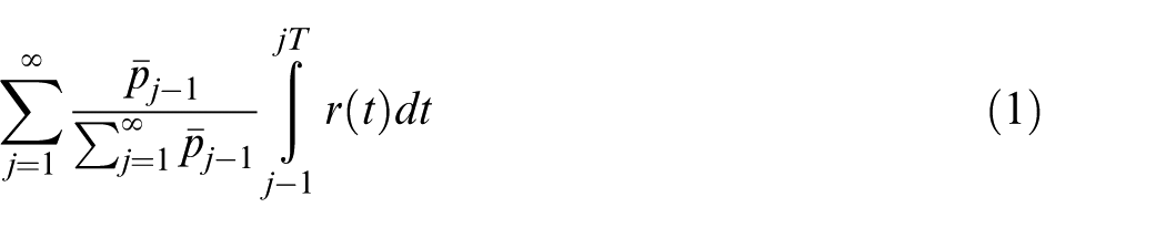
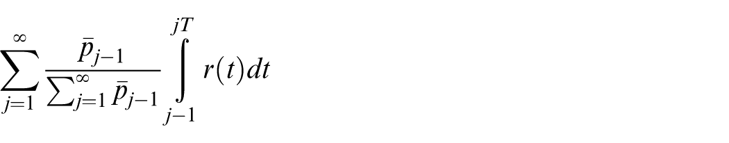
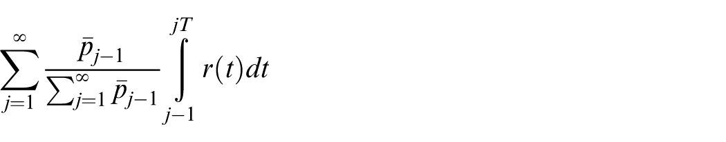
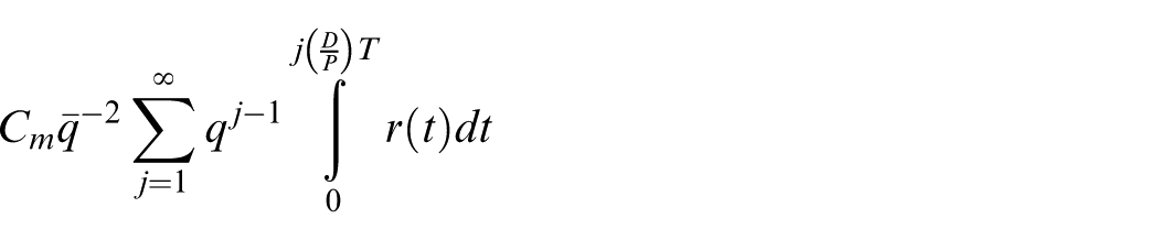
Furthermore, the expected minimal repair and backorder cost is
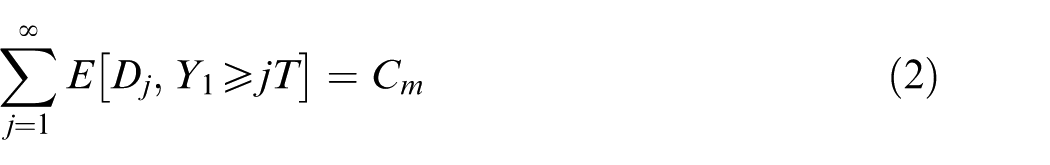
The expected failure number of periodic time T is
Proof
can be rewritten as
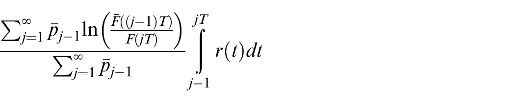
Forming T is finite,
Note that
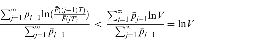
therefore, this series
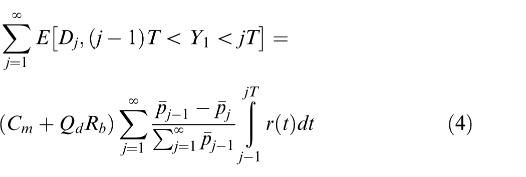
Then, we have
and
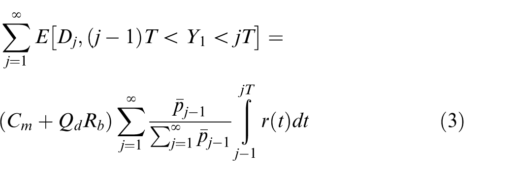
From equation (3), we get
The vendor’s total expected cost
The inventory level of this model is illustrated in Figure 1. Once the vendor receives an order, the vendor will produce the items immediately until quantity reach to mQ. The item delivered from vendor to buyer by each Q unit, and there are m lots will deliver in an inventory cycle. The average inventory of vendors can be evaluated as follows
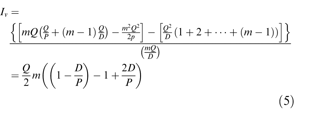
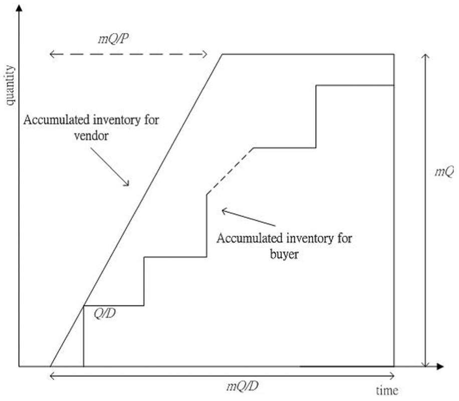
Inventory model for vendor.
Therefore, the vendor’s expected holding cost per year is
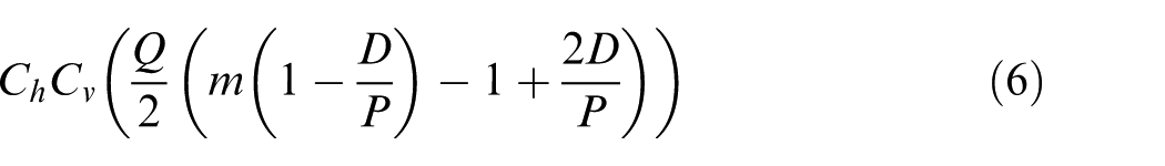
According to the assumptions and notations, the total expected annual cost for vendor is shown as below
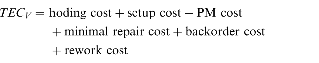
And the costs of vendors are derived as follows:
1. Holding cost
We have
and
2.
3.
4.
5.
Our production system of PM strategy is shown in Figure 2.
Production system of PM strategy.
The vendor’s total expected cost can be obtained from the above equation
The purchaser’s total expected cost

And the costs of vendor are illustrated as follows:
Ordering cost of each cycle is:
Holding cost:
And we have
And
Therefore, the buyer’s expected cost can be obtained from the above equation as follows
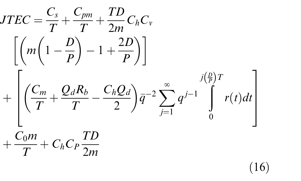
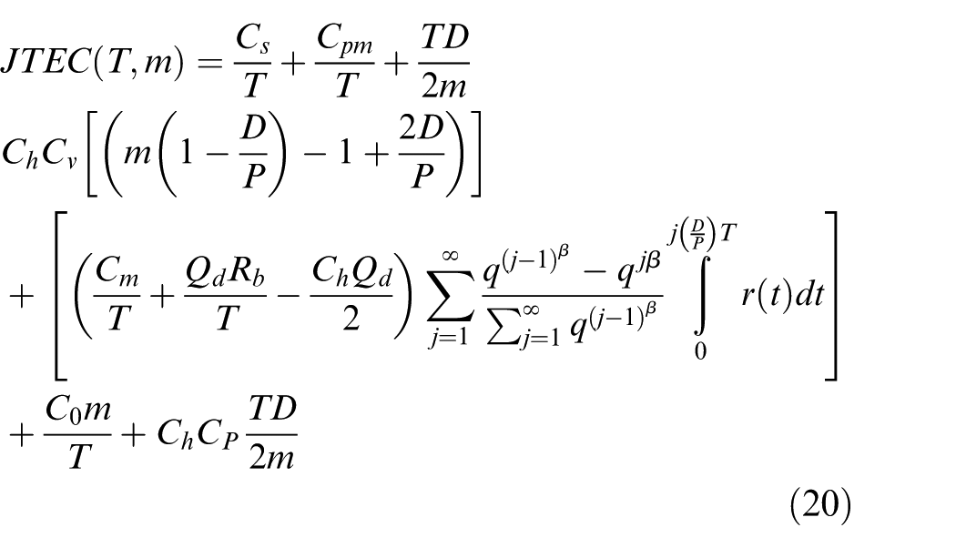
By adding the TECv and
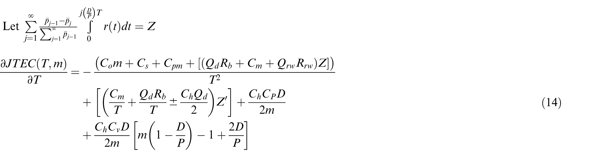
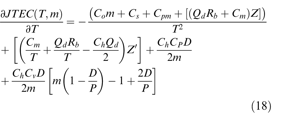
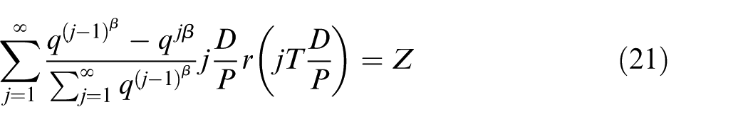
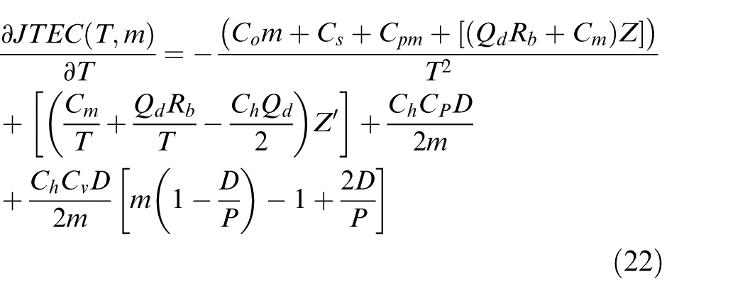
Taking the partial derivatives of joint total expected cost (JTEC) (T,m) to find the optimal inventory runs time T and m, there exist a finite and unique optimal solution to minimize JTEC
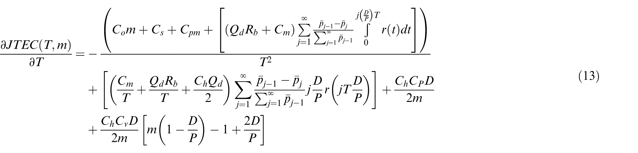
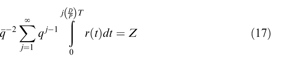
Let
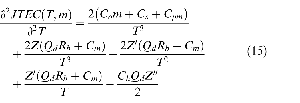
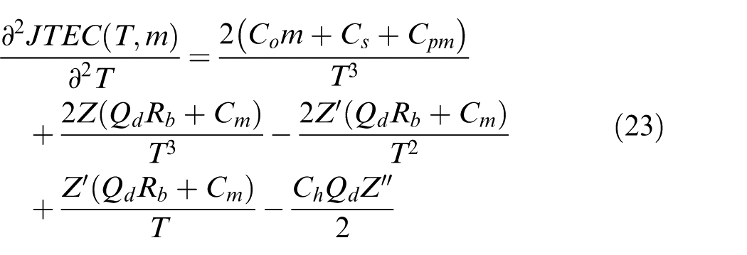
And we do second-order partial derivatives, if equation (22) > 0, then JTEC will exist a local minimal solution
Proof
See Appendix 2.
Probability model
Geometrical distribution
Here, a type II PM is performed as geometrical distribution.
This model is considered by Nakagawa.
So, JTEC will become
Let
And we do second-order partial derivatives, if equation (22) > 0, then JTEC will exist a local minimal solution

Proof
See Appendix 3.
Weibull distribution
In the Weibull distribution,
The breakdown cost is as follows
So, the JTEC will become
Let
And we do second-order partial derivatives, if equation (22) > 0, then JTEC will exist a local minimal solution
Proof
See Appendix 4.
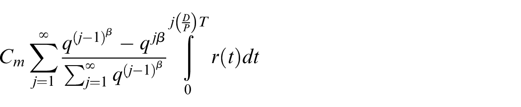
Learning effect
In this study, the learning effect is less noticeable while the number of PM times is becoming large. Therefore, the probability model is developed in the following discussion with the subsequent assumptions:
The breakdown costs are shown as follows based on the research by Liao et al. 23
So, the JTEC will become
Let
And we do second-order partial derivatives, if equation (22) > 0, then JTEC will exist a local minimal solution

Proof
See Appendix 5.
Numerical example
To illustrate the effectiveness of the models presented above, we examine a simplified numerical study. In this example, we are trying to find out an optimal value of T and m which is shown by the following four steps:
Step 1. Let m be equal to the minimum feasible value 1.
Step 2. Calculate T using relation.
Step 3. Calculate JTEC by embedding the last calculates T and m. If
Step 4. Find the minimum JTEC and the corresponding value of decision variables T and m as the optimal solution.
In order to illustrate the above solution procedure, we consider an inventory problem has the following data which are based on our discussion (Table 1) in order to represent more real-world situations.
Parameter setting.
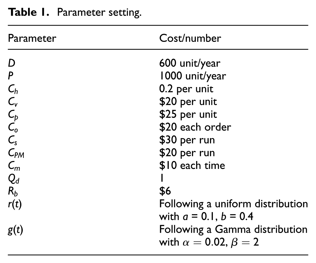
Numerical results sensitive analysis
In this part, we use the uniform and gamma distribution into the shot down rate, and the results are illustrated as follows.
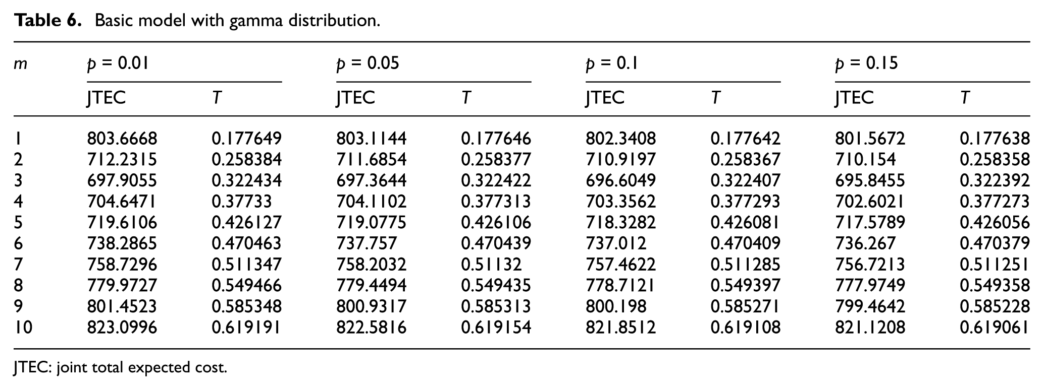
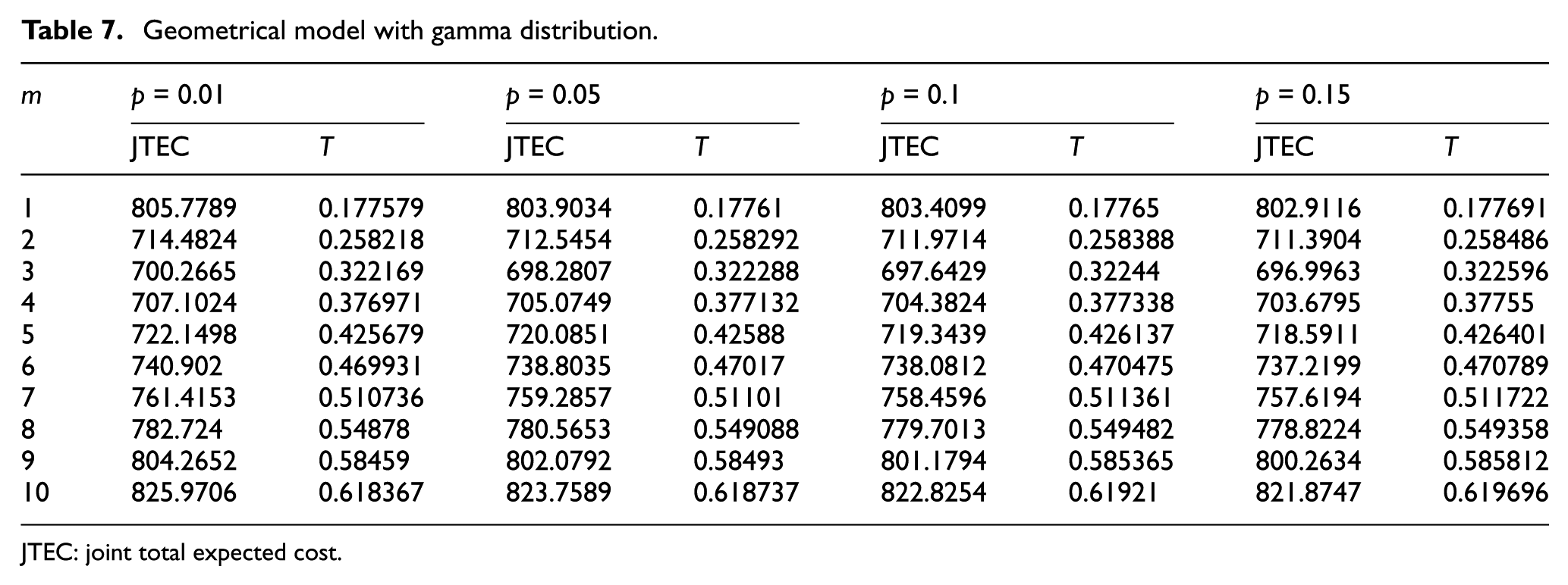
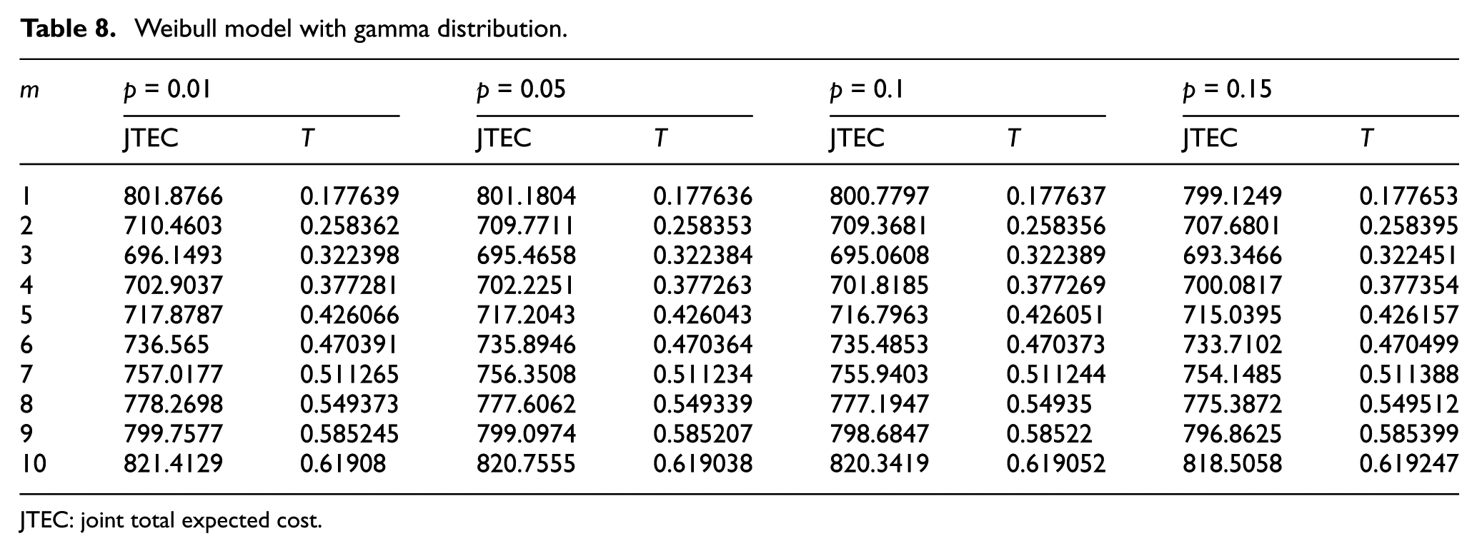
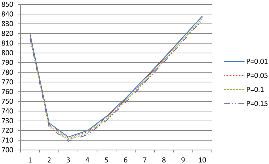
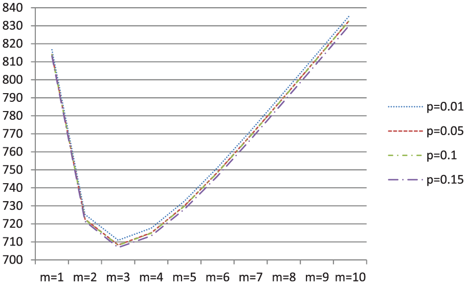
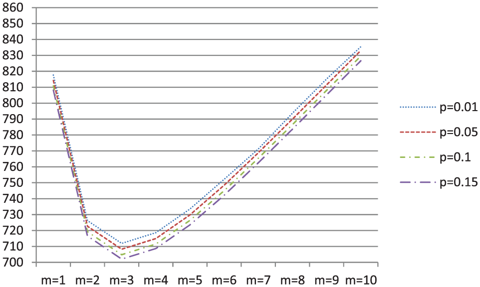
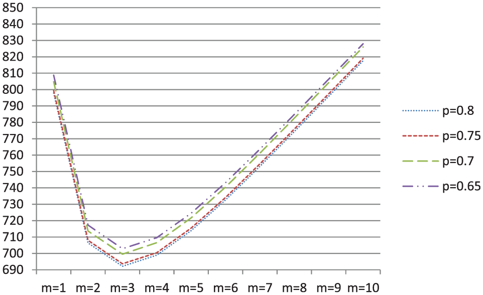
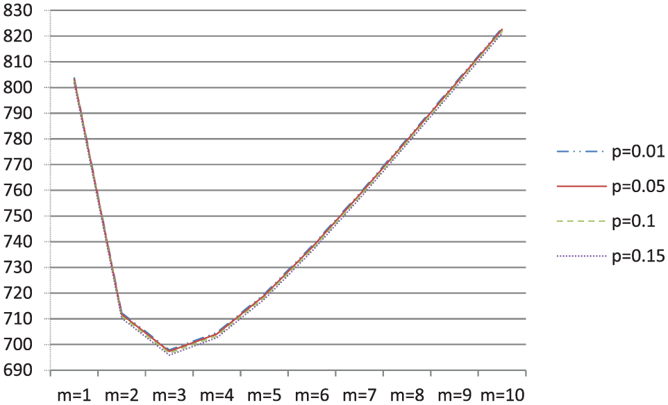
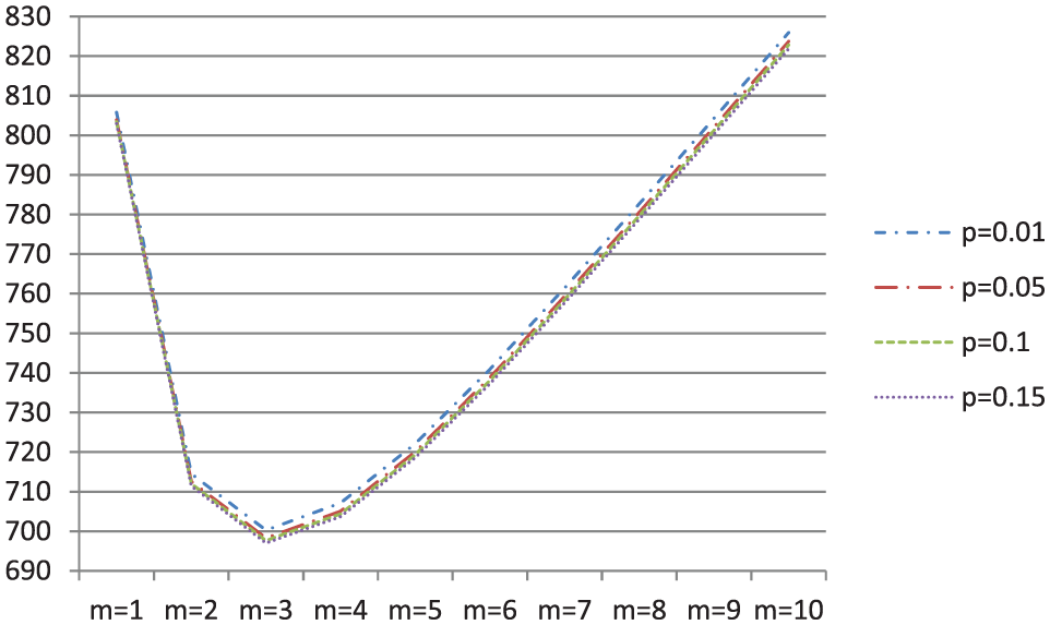
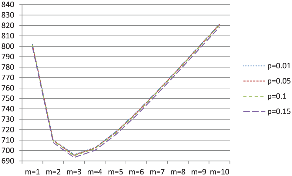
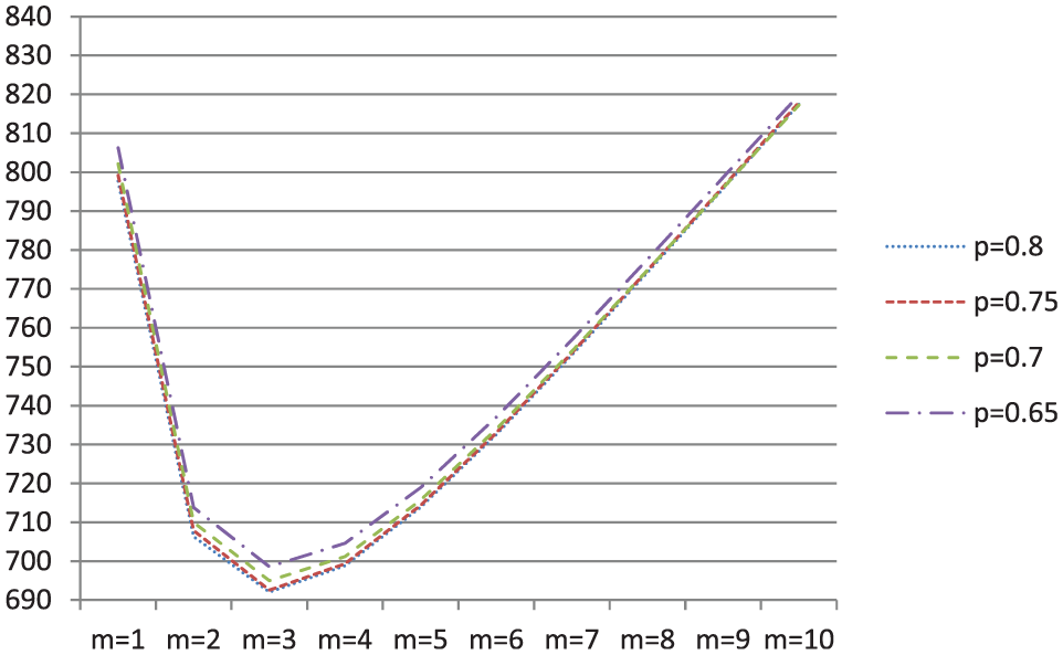
From Tables 2–9 and Figures 3–10, we can see when lot size m is 3; JTECs are decreasing. So we can find the corresponding value of the decision variables T and m as the optimal solution and the range of JTEC is 704–733.
Basic model with uniform distribution.
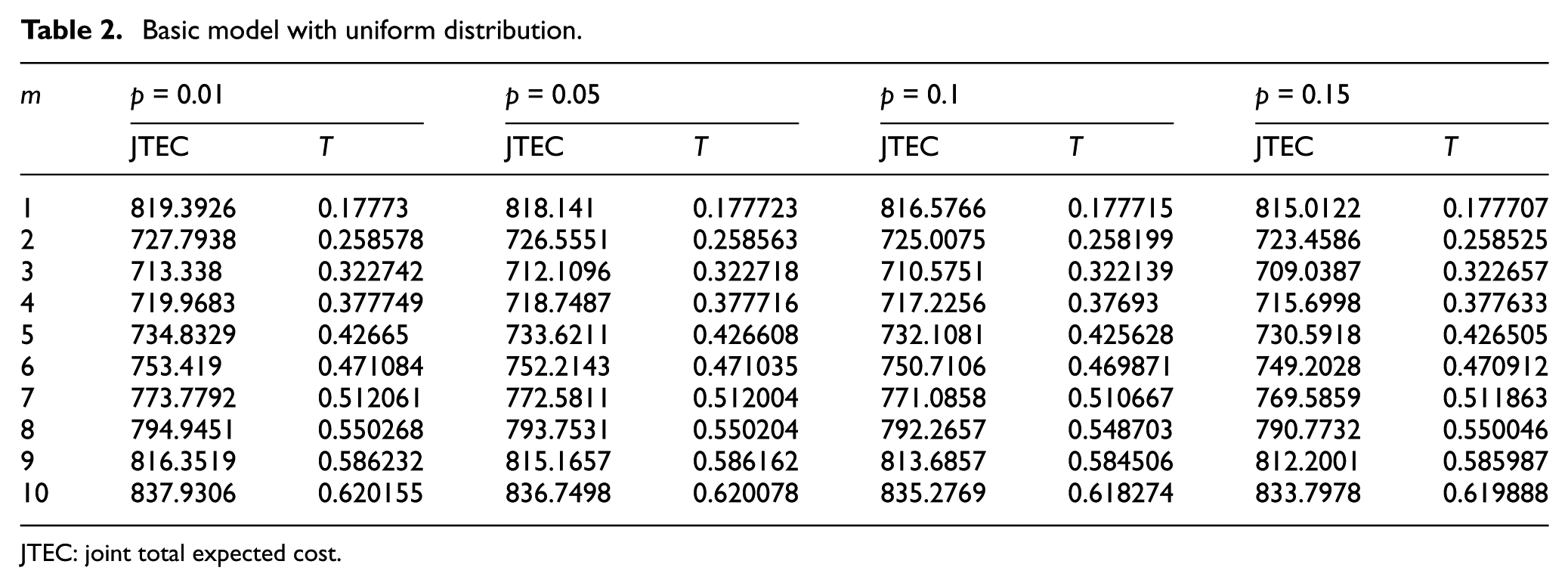
JTEC: joint total expected cost.
Geometrical model with uniform distribution.
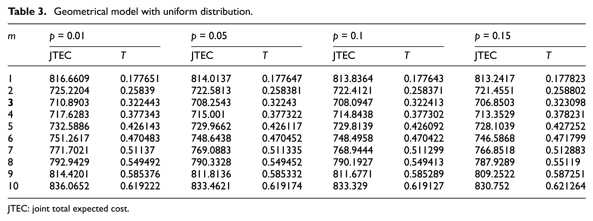
JTEC: joint total expected cost.
Weibull model with uniform distribution.
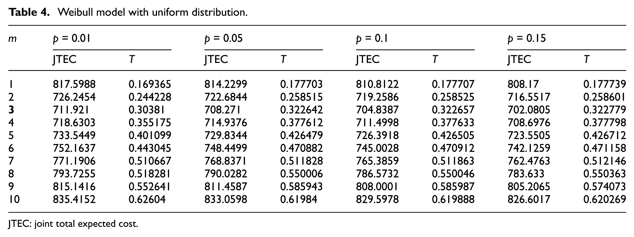
JTEC: joint total expected cost.
Learning curve model with uniform distribution.
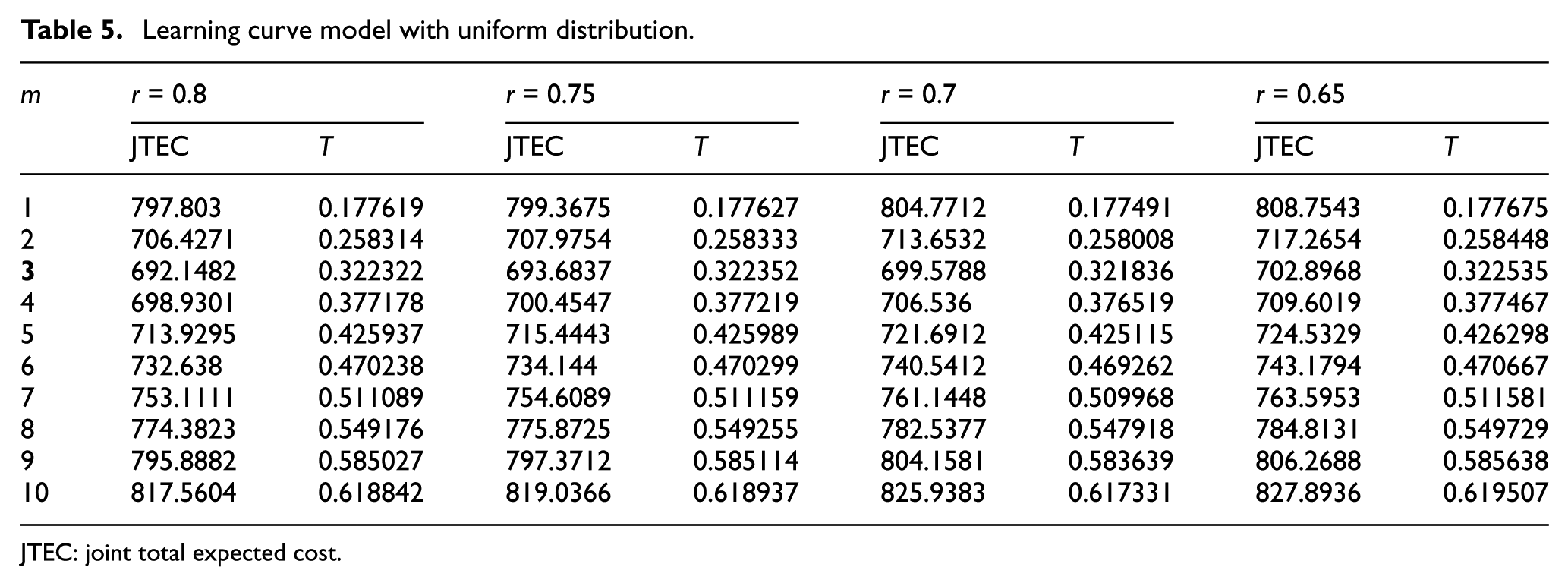
JTEC: joint total expected cost.
Basic model with gamma distribution.
JTEC: joint total expected cost.
Geometrical model with gamma distribution.
JTEC: joint total expected cost.
Weibull model with gamma distribution.
JTEC: joint total expected cost.
Learning curve model with gamma distribution.
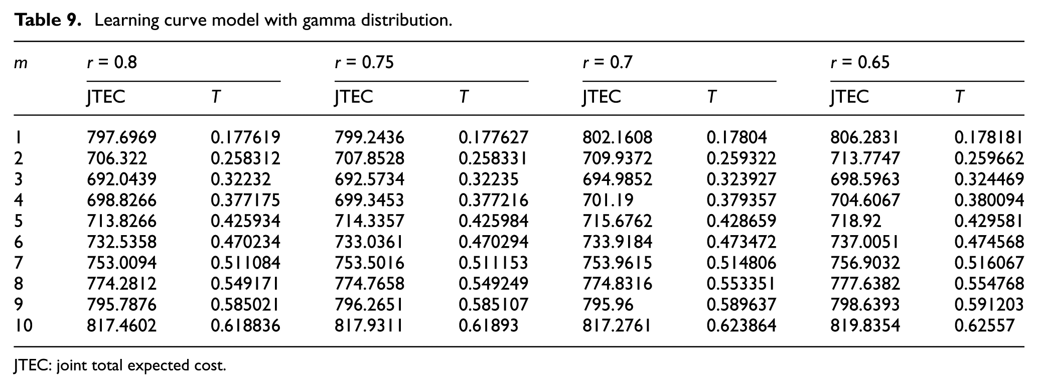
JTEC: joint total expected cost.
Basic model with uniform distribution.
Geometrical model with uniform distribution.
Weibull model with uniform distribution.
Learning curve model with uniform distribution.
Basic model with gamma distribution.
Geometrical model with gamma distribution.
Weibull model with gamma distribution.
Learning curve model with gamma distribution.
In the basic model, geometrical and Weibull with uniform and gamma distribution; when maintenance factor increases, the JTEC will decrease. In the learning curve model, the basic value of the maintenance factor differs from other models. If the maintenance factor decreases, the JTEC will increase.
Sensitive analysis
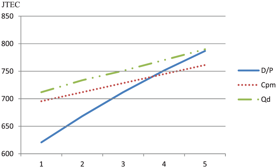
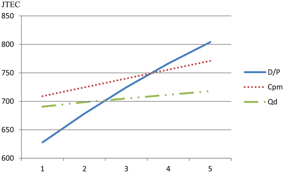
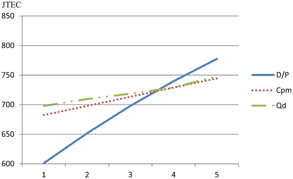
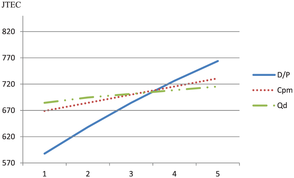
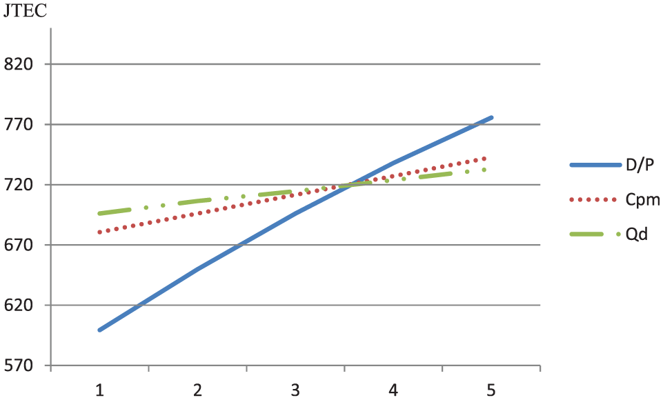
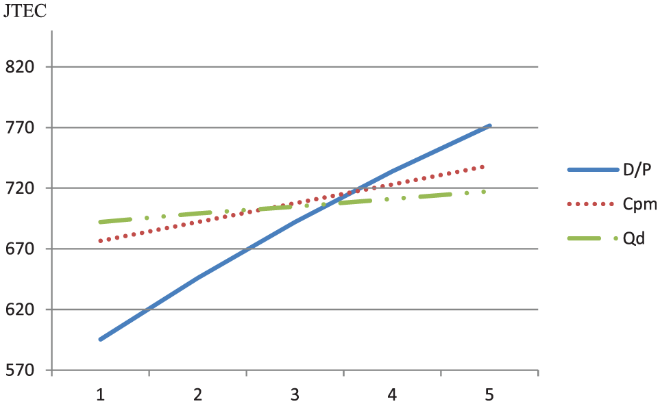
In this section, we apply the sensitive analysis to analyze our integrated inventory mode three key impact factors: D/P,
The abbreviations of eight cases.
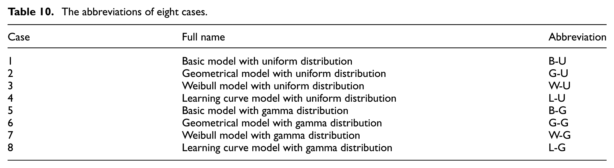
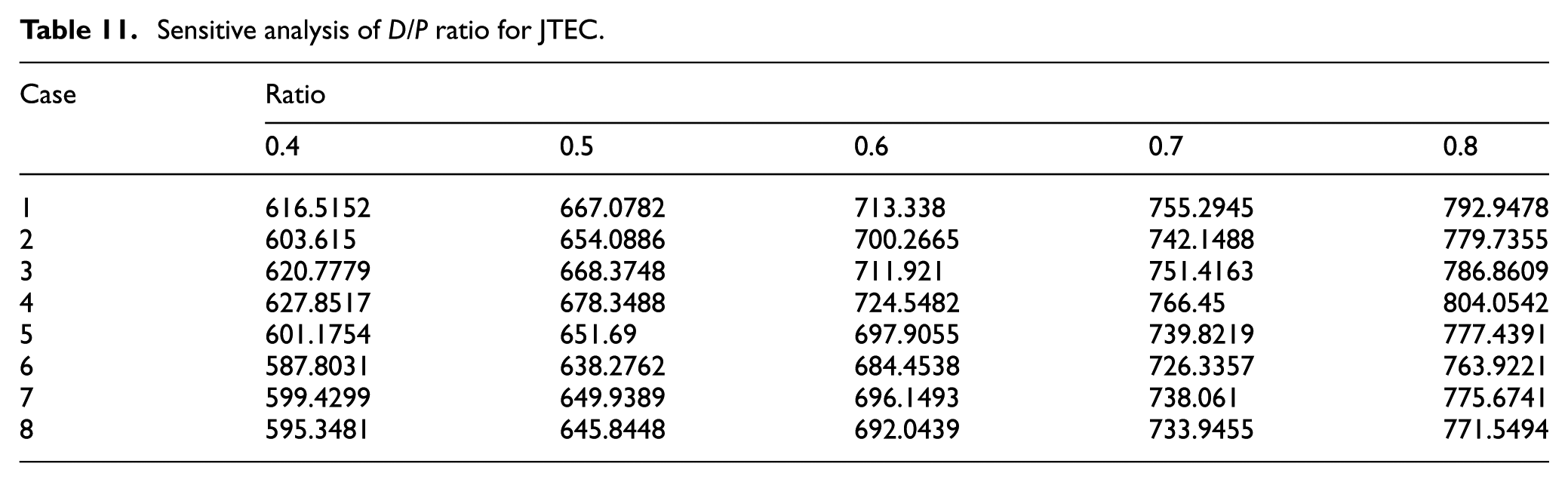
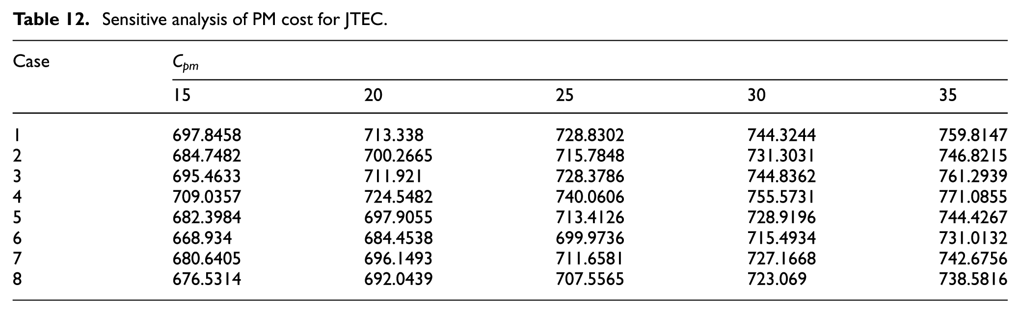
According to the results from Table 11, the joint total cost is increasing while the demand and production ratio D/P is increasing. That is because the D/P ratio influences the holding cost and purchase cost. Table 12 shows that when we increase the PM cost
Sensitive analysis of D/P ratio for JTEC.
Sensitive analysis of PM cost for JTEC.
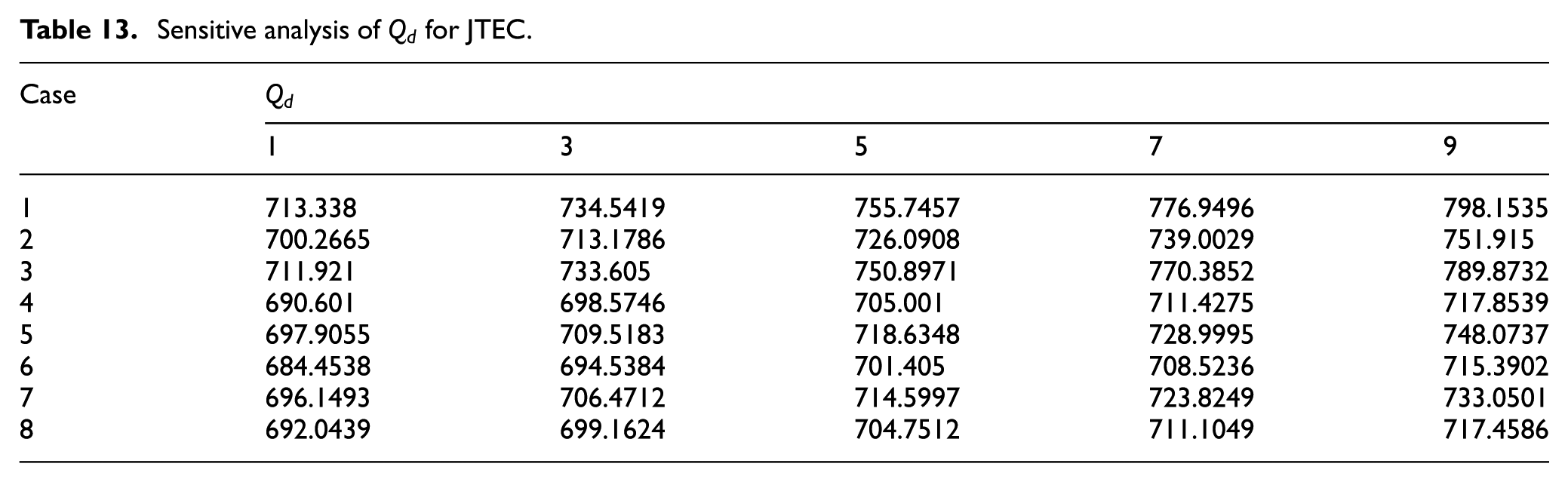
Then, Table 13 shows that when we increase the number of non-reworkable defective products
Sensitive analysis of
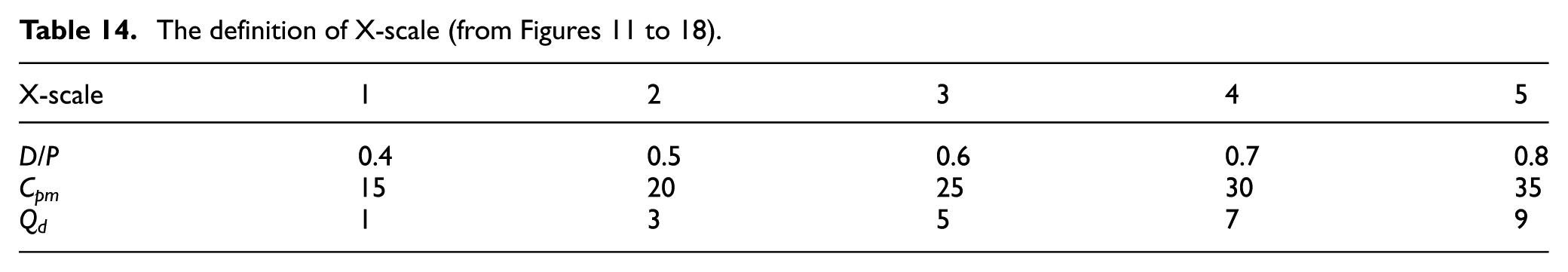
The definition of X-scale (from Figures 11 to 18).
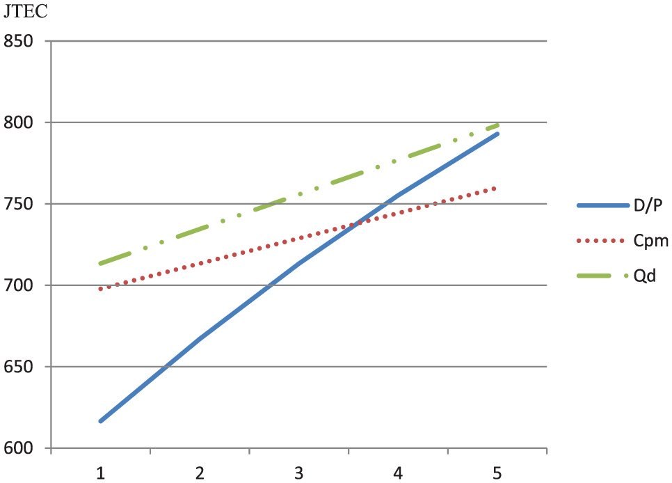
Sensitive analysis of basic model with uniform distribution.
Sensitive analysis of geo model with uniform distribution.
Sensitive analysis of Weibull model with uniform distribution.
Sensitive analysis of learning curve model with uniform distribution.
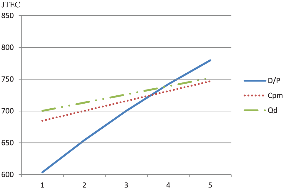
Sensitive analysis of basic model with gamma distribution.
Sensitive analysis of geo model with gamma distribution.
Sensitive analysis of Weibull model with gamma distribution.
Sensitive analysis of learning curve model with gamma distribution.
From Figures 11–18, we can see that among the three impact factors, the D/P ratio has the highest influence with integrated model.
Conclusion
Basically, in this article, we are considering the situation of both vendors and buyers which indicate that the buyer’s cycle is Q/D and the whole integrated cycle is DQ/m. In other words, our research extends past model based on the buyer’s ordering cycle which is different against Liao’s model. To sum up, this research focuses on the integrated inventory model development which has the difference of Liao’s EPQ model.
In this research, five of these findings are worth summarizing: (1) the analysis of PM strategy, production process’s fail and minimal repair; (2) the considerations of reworkable defective products at each failure and backorder with non-reworkable defective products at each failure during the production processes; (3) developing an integrated inventory model within the vendor’s inventory model and buyer’s inventory model; (4) the application of four PM probability and two shot down probability in our proposed model; and finally (5) providing an example to illustrate how the proposed model works. To sum up, we present the results of our integrated model with one vendor one buyer consideration and an effect of the modified production processes via the detailed numerical example.
Based on the results, the demand and production (D/P ratio) influences the holding cost and purchase cost and has the highest impact on the integrated model.
Future work will hopefully involve the real-world concern to our research which will be our main target. In addition, we do hope our research can be extended into more considerable areas such as multi-buyer or multi-vendor problems. Also we can apply more considerable variables such as PM time interval, permissible delay in payments and test error.
In spite of all the limitations of our research, we believe that the findings from our study are intriguing enough to encourage further research into the topic of an integrated inventory model.
Footnotes
Appendix 1
Appendix 2
Appendix 3
Appendix 4
Appendix 5
Declaration of Conflicting Interests
The author(s) declared no potential conflicts of interest with respect to the research, authorship, and/or publication of this article.
Funding
The author(s) received no financial support for the research, authorship, and/or publication of this article.