Sage Journals: Discover world-class research

Abstract

The purpose of this study was to characterize critical speed (CS) models for summarizing high-resolution speed-duration profiles from GPS tracking data obtained from soccer players. GPS data from 15 male NCAA Division I soccer players were collected during practices and games over a 6-week period. Moving averages of the speed data were computed for each file for duration windows spanning 0.1 to 600 seconds at 0.1-second resolution. Speed-duration profiles for each session and for the entire sampling period (“global”) were generated for each player by selecting the maximal mean speeds for each duration. Four models were fit to the profiles: the two-parameter CS (CS2) model, the three-parameter CS (CS3) model, the omni-domain speed-duration (OmSD) model, and the five-parameter logistic (5PL) model. The 5PL, CS3, and OmSD models exhibited similar goodness of fits, and all outperformed the CS2 model. Similar CS estimates were obtained for each model, whereas maximum speed (S_max) estimates were lower for OmSD compared to the 5PL. Players exhibited a range of parameter values for CS, D′, and S_max. S_max and CS estimated from session-specific speed-duration profiles were on average higher for games compared to practices. We conclude that CS models are useful for empirically describing speed-duration profiles and for assessing peak running demands for soccer practices and games. The proposed approach could help coaches design practice activities to better mimic game demands.

Keywords

Association football athlete monitoring global positioning system player tracking

Introduction

Designing effective training activities is a central task for sport coaches. Effective training sessions stimulate adaptations that improve the athlete's ability to meet the demands of competition. Sport scientists support coaches by quantifying the physical demands of training and competition. In field-based team sports such as soccer, player tracking technologies based on global positioning system (GPS), accelerometry, and video facilitate the unobtrusive collection of data that can be used to assess physical demands.^1–3 However, the magnitude and complexity of the data that results from these technologies presents a data science challenge within contemporary sport science.

The physical demands of field-based team-sports like soccer are operationalized in diverse ways. Locomotor variables such as total distance covered, average speed (also called “relative distance”), distances or time accumulated in different speed zones, and accelerations and decelerations are commonly measured.^1,2,4 More advanced “derived variables” such as metabolic power, player load, and exertion index use velocity and acceleration data to infer physiological demands.² While these measures are useful, opportunity exists to better leverage the data. Characterizing exercise intensity demands is a particular challenge. Existing measures such as relative distance and distance or time spent sprinting or in “high-speed running” are indices of intensity. However, most analyses to date focus on averaged or aggregate measures over prolonged epochs of time, such as entire practices or games, or game halves. This approach leads to an incomplete picture because bouts of play at the highest intensities are disproportionately consequential to athlete fatigue and training adaptations.⁵

Accordingly, peak locomotor demands, also called “maximal intensity periods,” “most demanding passages,” or “worse-case scenarios,”^5,6 are of interest to coaches and sport scientists. These demands are best characterized through rolling average approaches,^7–9 in which the locomotor variables are quantified for windows of time across the session. Typically, sliding windows of 1 to 15 minutes are applied.¹⁰ In the sport of soccer, peak running demands have been characterized for various ages, sexes, and playing levels.⁶ For example, the 1-, 3-, and 10-minute peak relative distances of professional male soccer players are approximately 200, 150, and 120 m/min, respectively.⁶ Such analyses are used to design training activities that mimic competition demands.^4,11–16

One limitation of research into peak demands is that data from only a few arbitrarily selected durations are typically presented, with 1, 3, 5, and 10-minute being the most common.⁶ In principle, it would be more informative to construct profiles with more durations, but doing so causes challenges with interpretability. This challenge can be addressed by using mathematical models, which efficiently summarize data with an equation featuring a few parameters. Indeed, speed-duration profiles for soccer and rugby athletes were summarized by fitting a power law equation^17–19 or a five-parameter logistic equation (5PL).²⁰ While effective for summarizing the data, both equations are empirical: their parameters lack physiological interpretability.

In endurance sports such as cycling, the relationship between the maximum sustainable power and duration, which is called the power profile, has been extensively studied.²¹ These profiles have been modeled using different forms of the critical power model.²² The original and simplest critical power (CP) model is the two-parameter CP model, which describes how the maximally sustainable power varies with durations ranging approximately from 2 to 30 minutes²³ (Equation (1)):

P (t) = \frac{W^{'}}{t} + CP

(1)

where t is the duration of the performance, P(t) is the power of the performance, and CP and W′ are physiologically interpretable model parameters.²⁴ CP was originally defined as the maximum power that can be sustained for prolonged durations without fatigue, but it is now recognized as the intensity demarcating the heavy and severe exercise intensity domains.²⁴ W′ can be defined as the mechanical work that can be supplied by finite processes distinct from those that support exercise at or below CP.^23,24 CP is physiologically interpreted as a measure of aerobic fitness while W′ is thought to largely (but not exclusively) reflect anaerobic work capacity.^23,24 Analogous critical speed (CS) models exist for sports in which power output is difficult to measure, such as running. The model parameters for the two-parameter CS (CS2) models are CS (m/s), which is the speed demarcating the heavy and severe exercise intensity domains, and D′ (m), the distance that can be supplied by finite processes distinct from those that support exercise at or below CS. CS2 models have been used to fit soccer speed-duration profiles spanning 1 to 600 seconds.^25,26 Three-parameter versions of CS models exist, including the three-parameter CS (CS3) model and the truncated version of the omni-domain speed-duration (OmSD) model, for which the third parameter is maximum speed (S_max).²² S_max can be interpreted as the theoretical maximum instantaneous sprint speed of the athlete. To our knowledge, three-parameter CS models have yet to be used for fitting speed-duration profiles from soccer players.

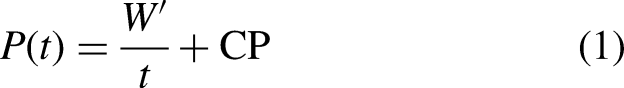
The purpose of this study was to generate and analyze high-resolution speed-duration profiles from GPS-based data from soccer players, and to test the ability of CS models to fit these profiles. Specifically, we compared the goodness-of-fits between CS models featuring three parameters, the CS2 model, and the empirical 5PL model. Given that the CS3 and OmSD models feature physiologically interpretable parameters (CS, D′, S_max), we hypothesized that they would provide equivalent or better goodness-of-fits than the 5PL model, despite the latter's two additional adjustable parameters, which make the 5PL more flexible and thus theoretically better able to fit data. We included the CS2 model in the analysis, which we hypothesized would exhibit lower goodness-of-fits owing to its fewer parameters, to evaluate the benefit that the third parameter in the CS3 and OmSD models would provide.

The paper is structured as follows. In the “Methods” section, we describe the data provenance and processing, the models and rationale for choosing them, and the modeling and statistical procedures. In the “Results” section, we present analyses of data quality, model goodness of fits, and the practice versus game comparisons. In the “Discussion” section, we interpret the results, discuss limitations, and propose implications for training activity design.

Methods

Participants and ethical approval

Fifteen healthy male players (height: 179 ± 5.9 cm; mass: 75.5 ± 4.7 kg) of the Seattle University NCAA Division I soccer team participated in this study. Three players were forwards, seven were midfielders, four were defenders, and one player played both midfield and defence. Ethical approval for the proposed studies was obtained from the Office of Research Ethics at Simon Fraser University and Seattle University. Permission to conduct the study was granted from the team.

Data collection

Data were collected by the team staff members as part of the team's daily training routine; the data were therefore purely observational. GPS-based tracking devices were inserted into custom-made pouches in the players’ jerseys located between the scapulae. Each player was assigned the same unit for the entire collection period to circumvent potential inter-unit variability effects. Data were collected from each of the players for all matches and training sessions during August and September 2019. Forty-two sessions were completed, seven of which were matches and the remainder practices. On average, players participated in 33 ± 6.1 (mean ± SD; range: 16–38) of the 42 sessions, which consisted of 27 ± 4.8 practices and 5 ± 1.6 games.

Speed-duration data were collected using a GPS-based tracking system (SPT2, Australia; 10 Hz). The validity of this system was previously evaluated. In comparison to radar-based measurement, the system exhibited a root-mean-square difference (RMSD) of 0.84 m s⁻¹ and a coefficient of variation (CV) of 11.8%,²⁷ which was interpreted as strong overall validity. In addition, the inter-unit reliability of the system was also examined and was found to have a RMSD of 0.70 m s⁻¹, and a CV of 9.0%.²⁷

Data processing

All computations were performed using R software.²⁸ We developed code that extracted and processed the data as follows. First, we split the data into sessions, removed “NA” values, and excluded data with low quality GPS signal (i.e. horizontal dilution of precision [HDOP] > 2) and unrealistically high speeds (i.e. ∼43 km h⁻¹ or 12 m s⁻¹). Thereafter, for each dataset, we applied functions that calculated the moving averages for the speed data for durations from 0.1 to 600 seconds, in 0.1 seconds increments. The maximum observed mean speeds for each duration define the athlete's speed-duration profile. Speed-duration profiles were generated for each session for each athlete (“session-specific speed-duration profiles”) and across each athlete's total data collected over the 6 weeks (“global speed-duration profiles”).

Data modeling

We fit four models to the speed-duration profiles, the 5PL and three models from the critical-speed model family (CS2, CS3, and truncated OmSD; Table 1). The rationale for choosing these models was as follows. The CS2 model has been used to fit soccer speed-duration profiles,^25,26 but goodness-of-fit metrics were not reported. In addition, the CS2 features only two adjustable parameters and trends to infinity as duration approaches zero, which is physiologically unrealistic. We therefore hypothesized that the CS2 would perform the least well for fitting speed-duration profiles. By contrast, the 5PL featured superior goodness-of-fits to speed-duration profiles compared to several other empirical models,²⁰ such that it can be considered the current gold-standard model. The 5PL model features five adjustable parameters: the upper asymptote (d), lower asymptote (c), inflection point (b), exponent (f), and decrease rate (a) (Table 1). While the 5PL may work well, modeling best practice emphasizes model parsimony, which means selecting the model with the fewest number of adjustable parameters that satisfactorily fits the data. In addition, the 5PL model is empirical, whereas it is preferred that model parameters be physiologically interpretable.

Table 1.

Model parameters and equations.

Model	Critical speed-related parameter	D′-related parameter	Maximal speed-related parameter	Additional parameters and meanings	Model equations
CS2²³	CS	D′	n/a		$S (t) = \frac{D^{'}}{t} + CS$
5PL²⁰	c	n/a	d	a = decrease rate b = inflection point f = exponent	$S (t) = c + \frac{d - c}{{1 + e^{- a [\log_{10} (t) - b]}}^{f}}$
CS3^23,29	CS	D′	S _max		$S (t) = \frac{D^{'}}{t + (\frac{D^{'}}{S_{\max} - C S})} + CS$
OmSD²²	CS	D′	S _max		$S (t) = \frac{D^{'}}{t} [1 - e^{- t (\frac{S_{\max} - CS}{D^{'}})}] + CS$ , t < 1800 seconds

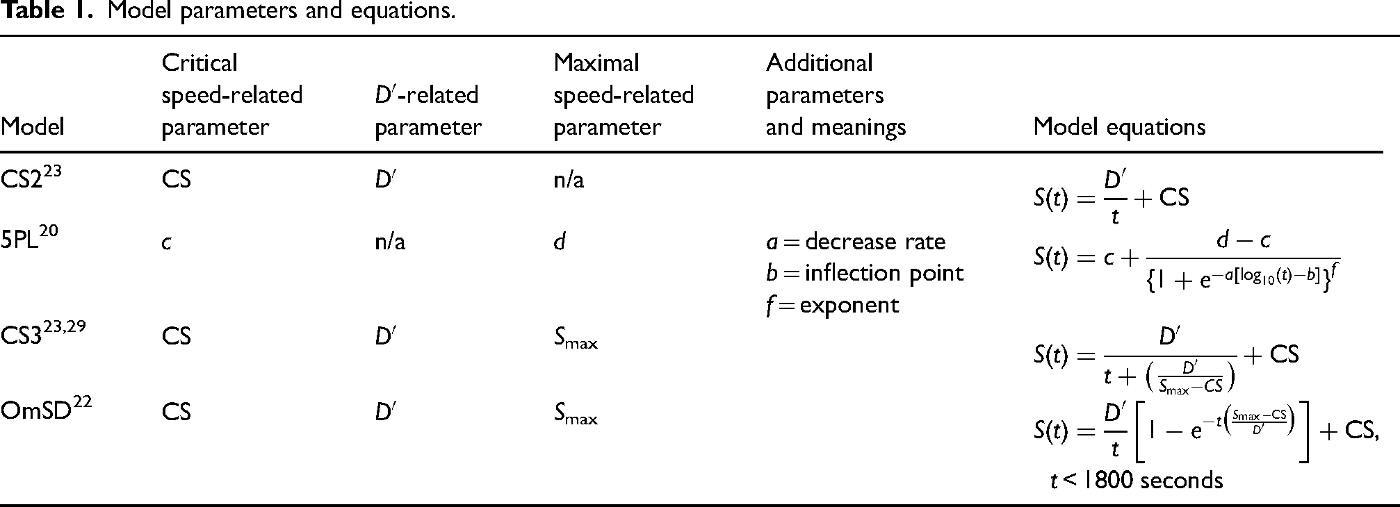
CS models with three adjustable physiologically interpretable parameters such as the CS3²³ and the truncated OmSD²² may be effective for modeling GPS-based speed-duration profiles. In addition to CS and D′, both models feature the parameter S_max, which represents the maximum instantaneous speed (Table 1). Both models should therefore be valid for speeds at very short durations, unlike the CS2 model. The truncated version of the OmSD model, which applies to durations of 30 minutes or less, is similar to the CS3 model (Table 1) but offers improved theoretical treatment of D′.²²

To fit the models, we used nonlinear regression by applying the “nlsLM” function from the “minpack.lm” package in R. The fits were optimized using the Levenberg–Marquardt algorithm to minimize the residual sum-of-squares (RSS). The R code used to process the data and fit the models is freely available in the following GitHub repository: https://github.com/aaronzpearson/critspeed. The model parameter values were bounded to ensure realistic estimates would be obtained.

Operational definitions and hypothesis tests

We operationally defined model goodness-of-fits as the root mean square error (RMSE), the Akaike information criterion (AIC) and the Bayesian information criterion (BIC).^30,31 Models with the lowest values for RMSE, AIC, and BIC would be interpreted to exhibit the best goodness-of-fits. RMSE is calculated as the standard deviation (SD) of the model residuals. In general, the RMSE will be lower for models that have more parameters, because such models are more flexible. The AIC is calculated as the difference between the maximum value of the likelihood function for the model and a corresponding penalty term calculated from the number of estimated parameters in the model.³¹ BIC is similar to the AIC except its penalty term depends additionally on the sample size.³²

To statistically test the research hypotheses, we applied linear mixed-effects models. Model goodness-of-fits were assessed by a mixed-effects model featuring the RMSE, AIC, or the BIC as the response variable and the model types and player ID as explanatory variables. The model types and player ID terms were designated as fixed and random effects, respectively. The CS, D′, and S_max estimates from each model were likewise compared using mixed-effects models featuring the parameter as the response variable and model types and player ID as the explanatory variables.

The mixed-effects models were fit using the “lmer” function from the “lme4” package in R. Following the omnibus test, pairwise comparisons between the CS models were made using the “emmeans” function. To assess between-player differences in the speed-duration profiles, we performed a likelihood ratio test on the player ID random-effect terms from the mixed-effects models for the model parameters using the “ranova” function in R. The familywise level of significance, α, was set at 0.05 and multiple comparisons were controlled by the Tukey method. Residual analyses were performed to evaluate the mixed-effects model assumptions.

Two-tailed Wilcoxon signed rank tests were performed to test the differences in the values of CS, D′, and S_max between practices and games.

Results

High-resolution speed-duration profiles

The dataset consisted of approximately 36 × 10⁶ data points (approximately 2 hours per session × 10 Hz sampling frequency × 33 sessions × 15 players). The computations to generate the speed-duration profiles for each player from all 42 sessions took less than 1 minute per player, using a Windows 10 computer with Intel i5-4300U CPU @ 1.90 GHz 2.49 GHz and 12.0 GB RAM. The code for these computations was implemented by independent coders in R and Python, and identical results were obtained. The R code was then developed to publication standard. The speed-duration profiles for each player are included as Supplemental Spreadsheet File.

Plots of the speed-duration profiles demonstrated curvilinear decreasing trends whose lower limits appeared to approach a horizontal asymptote (Figure 1(a)). In general, segments of maximal mean speeds across several durations were obtained from the same GPS file, with both practices and games featured (Figure 1(b) and (c)). Some profiles featured “bumps” in which the maximal mean speeds for longer durations were higher than those for shorter durations (Figure 1(d)).

Figure 1.

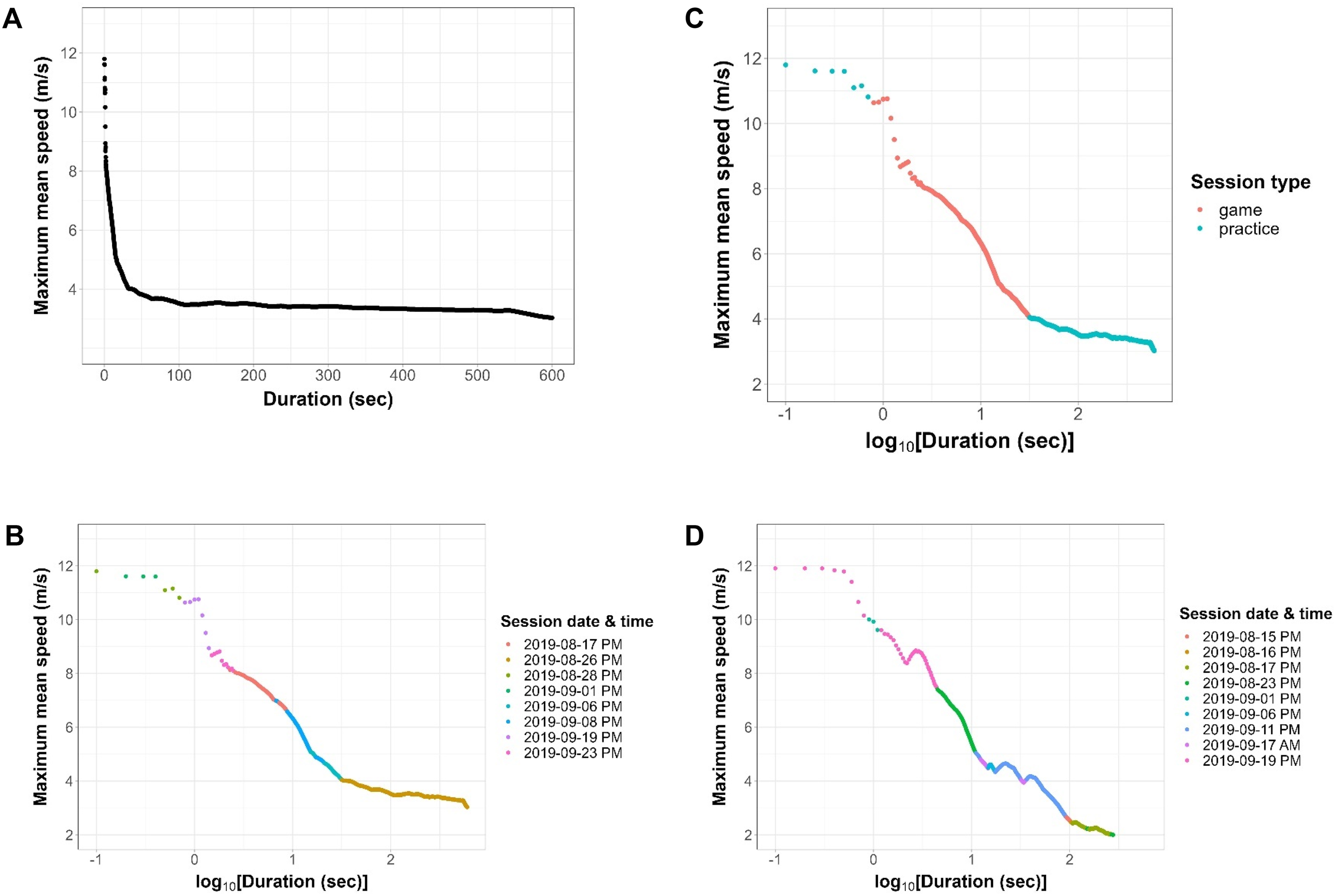
High-resolution speed-duration profiles from soccer players (panels a–c, ID = 731066; panel d, ID = 279462). (a) Representative speed-duration profile. The maximum observed mean speeds (m/s) exerted by the player across all sessions are plotted against their corresponding durations (in seconds, on a linear scale). (b) The same speed-duration profile as in panel a but plotted on a base-10 log scale and with the data points color-coded according to the session date and time in which they were observed. (c) The same speed-duration plot as in panel b but with the data points color-coded according to the session type (practice or game) in which they were observed. (d) A “bumpy” speed-duration profile plotted on a base-10 log scale and with the data points color-coded according to the session date and time in which they were observed.

To describe the peak running demands exerted by the players, we extracted the maximum mean speeds from the speed-duration profiles for the 60, 180, 360, and 600 seconds durations (Table 2). The maximal mean speeds decreased from 3.60 to 2.17 m/s from 60 to 600 seconds, respectively (Table 2).

Table 2.

Descriptive statistics [mean, standard deviation (SD), 95% confidence intervals (CI)] for the maximal mean speeds for the players (N = 15) across all sessions.

Duration (s)	Mean (m/s) (m/min)	SD (m/s) (m/min)	95% CI (upper, lower) (m/s) (m/min)
60	3.60 216	0.38 23	(3.54, 3.65) (213, 219)
180	2.56 154	0.32 19	(2.51, 2.61) (151, 156)
300	2.32 139	0.33 20	(2.28, 2.37) (137, 142)
600	2.17 130	0.27 16	(2.13, 2.21) (128, 132)

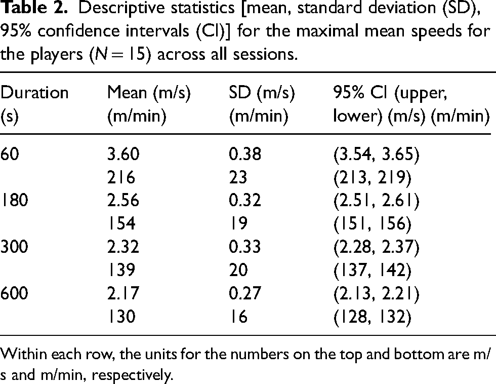
Within each row, the units for the numbers on the top and bottom are m/s and m/min, respectively.

Model parameter estimates

We first fit the four models to the global datasets with durations spanning 0 to 600 seconds. While the fits were qualitatively satisfactory for most of the data, we observed consistent departures of the models from the data at the shortest durations (<1 second; Figure 2(a) and (b) and Supplemental Figure 1). We therefore truncated the speed-duration profiles to 2 to 600 s and modeled these data (Figures 2(c) and 3). We observed satisfactory qualitative fits of the 5PL, CS3, and OmSD models to the data (Figures 2(c) and 3), whereas the CS2 demonstrated clear lack of fit (Figure 2). Model parameter values and goodness-of-fit metrics for each player are reported in Supplemental Tables S1 and S2.

Figure 2.

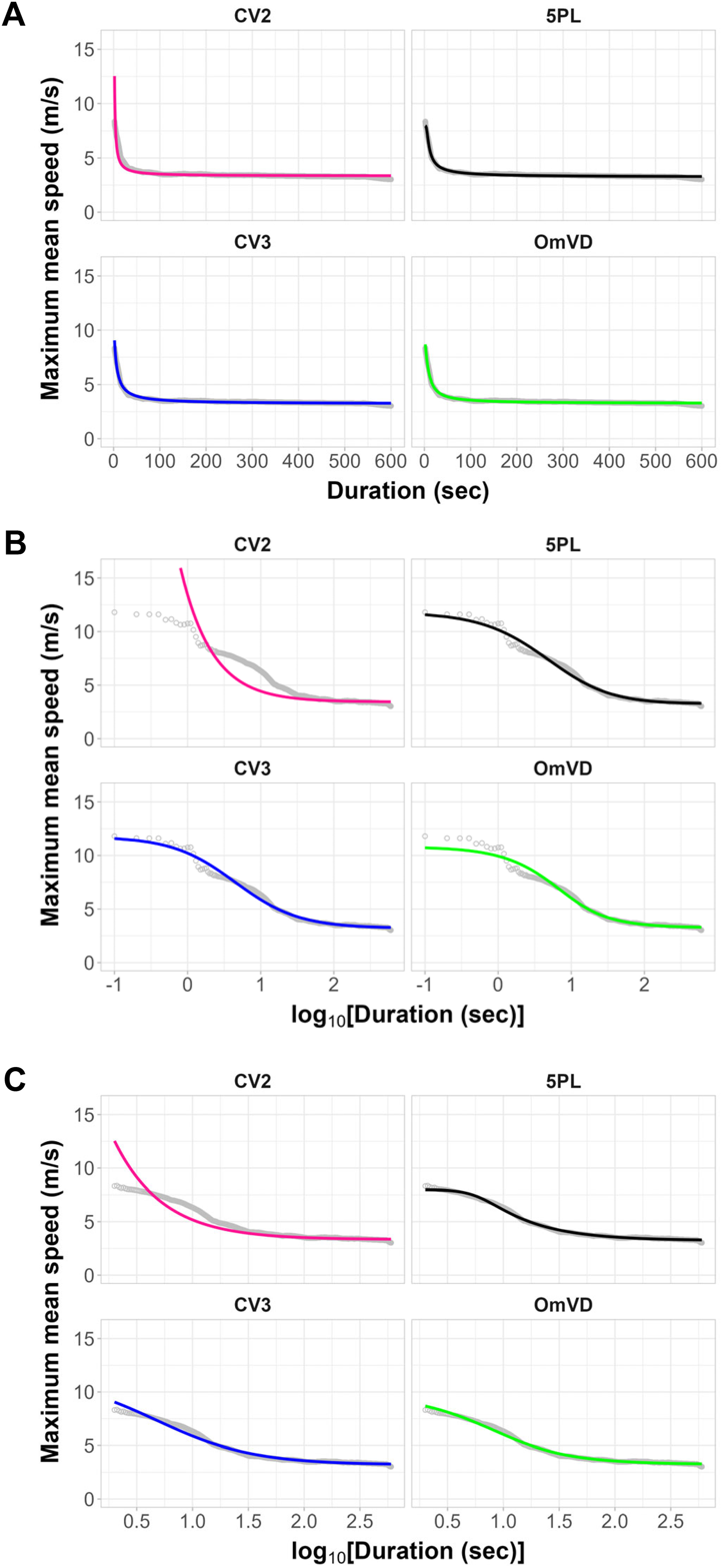
Representative speed-duration profiles for one player (ID = 731066) fitted by the CS2, CS3, 5PL, and OmSD models. (a) The independent variable, duration (seconds), is plotted on a linear scale. (b) Duration is plotted on a base-10 log scale. (c) Speed-duration profiles and model fits for truncated data (2–600 seconds).

Figure 3.

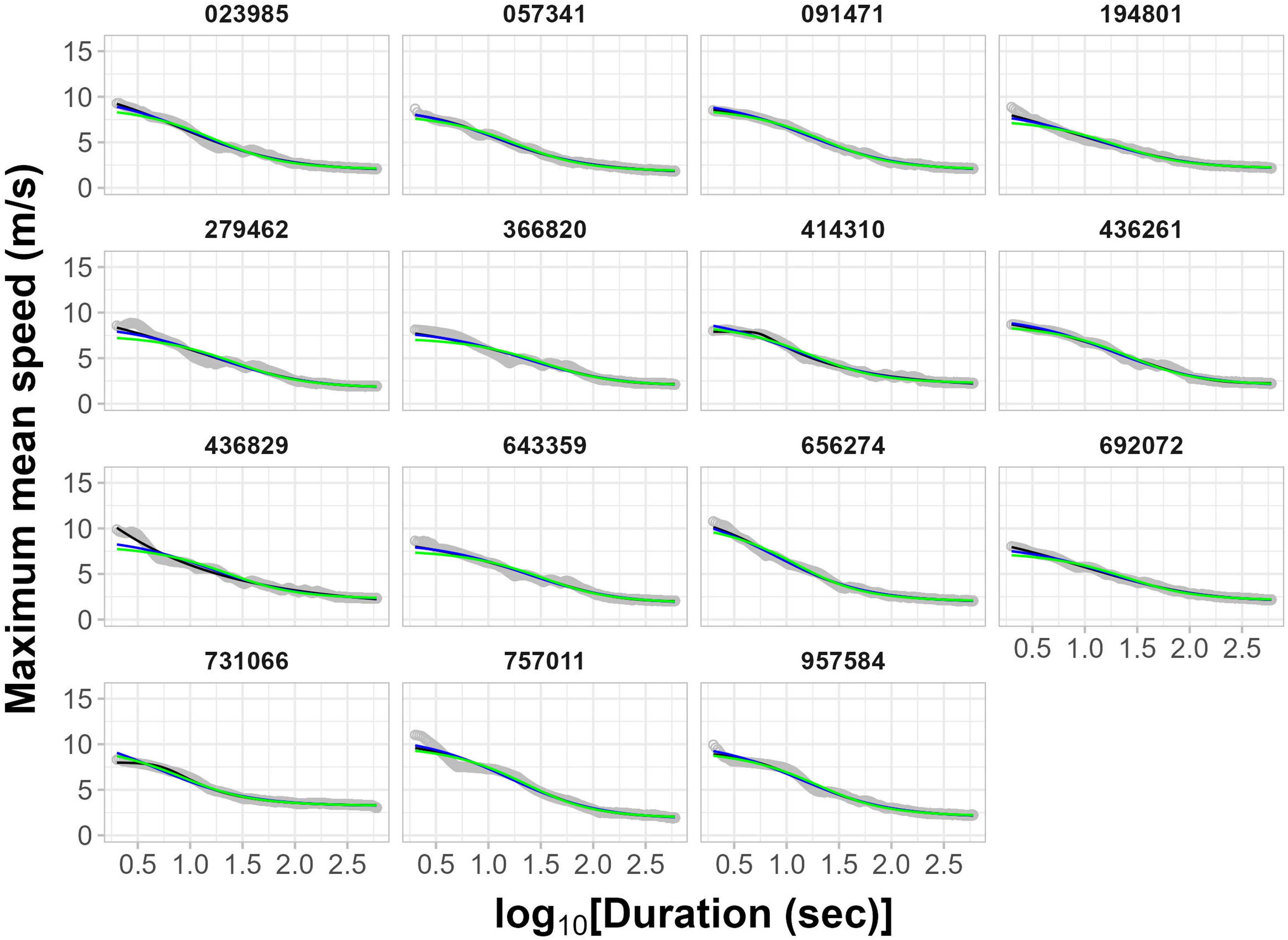
Plots of the 5PL (black), CS3 (blue), and OmSD (green) model fits of the speed-duration profiles for each player for 2–600 seconds data.

For the model parameter estimates, the four models returned CS estimates of approximately 2 m/s (Table 3). The CS2 estimates were statistically higher than those of the other models, whereas the CS estimates from the CS3, 5PL, and OmSD were not statistically different (Table 3). S_max estimates were obtained from the 5PL, CS3, and OmSD models, with the mean values of each decreasing from 10.2, 9.6, and 8.6 m/s, respectively (Table 3), with the OmSD being statistically lower than the 5PL (P = 0.0017). This ordering of S_max estimates was generally consistent when performed for each player, although S_max estimates from CS3 models were the highest for some players (Supplemental Table S1). D′ estimates were obtained from the CS3 and OmSD models, and their mean values across all players were 106 and 79 m, respectively (Table 3).

Table 3.

Summary data for model parameters and goodness-of-fits for the global speed-duration profiles for each player (N = 15).

Model	Model parameter values			Goodness-of-fit metrics
Model	CS (m/s)	D′ (m)	S_max (m/s)	RMSE	AIC	BIC
CS2	2.4 ± 0.3^a (2.1, 3.3)	26.0 ± 3.4 (18, 33)	NA	0.44 ± 0.10^a	6800 ± 3100^a	6800 ± 3100^a
5PL	2.0 ± 0.4 (1.3, 3.2)	NA	10.2 ± 1.5 (7.9, 12.0)	0.09 ± 0.03	−12,100 ± 4400	−12,000 ± 4000
	a −2.01 ± 2.66 (−0.43, −8.99)	b 5.69 ± 4.90 (0.18, 12.9)	f 50.1 ± 83.9 (0.053, 238)
CS3	2.0 ± 0.4 (1.7, 3.2)	106 ± 29^b (39, 150)	9.6 ± 1.2 (8.1, 12.0)	0.11 ± 0.04	−10,600 ± 4600	−10,500 ± 4600
OmSD	2.1 ± 0.4 (1.7, 3.2)	79 ± 21^b,c (32, 111)	8.6 ± 1.0^d (7.3, 10.7)	0.12 ± 0.04	−9100 ± 4000	−9100 ± 4000

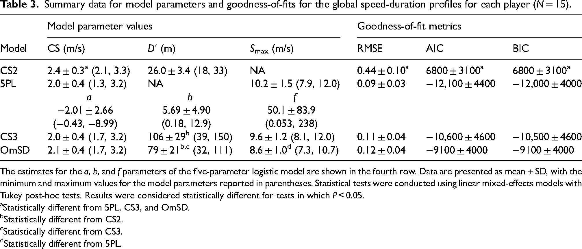
The estimates for the a, b, and f parameters of the five-parameter logistic model are shown in the fourth row. Data are presented as mean ± SD, with the minimum and maximum values for the model parameters reported in parentheses. Statistical tests were conducted using linear mixed-effects models with Tukey post-hoc tests. Results were considered statistically different for tests in which P < 0.05.

Statistically different from 5PL, CS3, and OmSD.

Statistically different from CS2.

Statistically different from CS3.

Statistically different from 5PL.

Differences between the players’ speed-duration profiles and the corresponding models were evident (Figure 3). The player-specific values for CS, D′, and S_max varied (Supplemental Tables S1 and S2), leading to a range of values being observed (Table 3). These observations were supported by the statistically significant likelihood ratio tests for the Player ID random-effect terms from the mixed-effects models for CS and D′ (CS: χ² = 54, P = 2 × 10⁻¹³; D′: χ² = 12, P = 4 × 10⁻⁴).

Goodness-of-fit metrics

The CS2 model exhibited the highest goodness-of-fit values, by far, of the four models, with mean RMSE, AIC, and BIC values of 0.44, 6800, and 6800, respectively (Table 3). The differences in values between CS2 and all other models were statistically significant (Table 3). The differences between the goodness-of-fits of the other models were not statistically significant. Their ordering from highest to lowest goodness-of-fit was 5PL, CS3, and OmSD (Table 3).

Residual plots (Supplemental Figure S2) showed that the residuals for all models exhibited systematic patterns as a function of the predicted values (Supplemental Figure S2A), departure from normal distribution (Supplemental Figure S2B), and autocorrelation (Supplemental Figure S2C). The patterns of the residuals were similar for CS3, OmSD, and 5PL models, but their values featured slight quantitative differences (Supplemental Figure S2). The residual magnitudes were highest for CS2 and exhibited distinct trends compared to those from the other models (Supplemental Figure S2). The highest discrepancies between the models and data occurred at the shortest durations/highest speeds (Supplemental Figure S2A). The trends observed in Supplemental Figure S2 plots were consistent across all players.

Models of session-specific speed-duration profiles reveal differences between practices and games

We fit the CS3 model to session-specific speed-duration profiles computed for each player from all the sessions that each completed. We color-coded the model plots for games and practices, and noticed clustering of the profiles for games towards the top for some players (Figure 4(a); e.g., player ID 091471, 643359, and 731066). The CS and S_max parameters from games were statistically higher than those from practices, while no difference was detected for D′ (Figure 4(b)). Specifically, the CS for games and practices were 1.6 ± 0.5 and 1.3 ± 0.4 m/s, respectively (W = 11,389, P = 2 × 10⁻⁶), the S_max values were 7.6 ± 1.7 and 6.7 ± 1.3 m/s (W = 10,154, P = 5 × 10⁻⁹), and the D′ values were 52.3 ± 44.2 and 53.3 ± 41.7 m (W = 16,180, P = 0.57).

Figure 4.

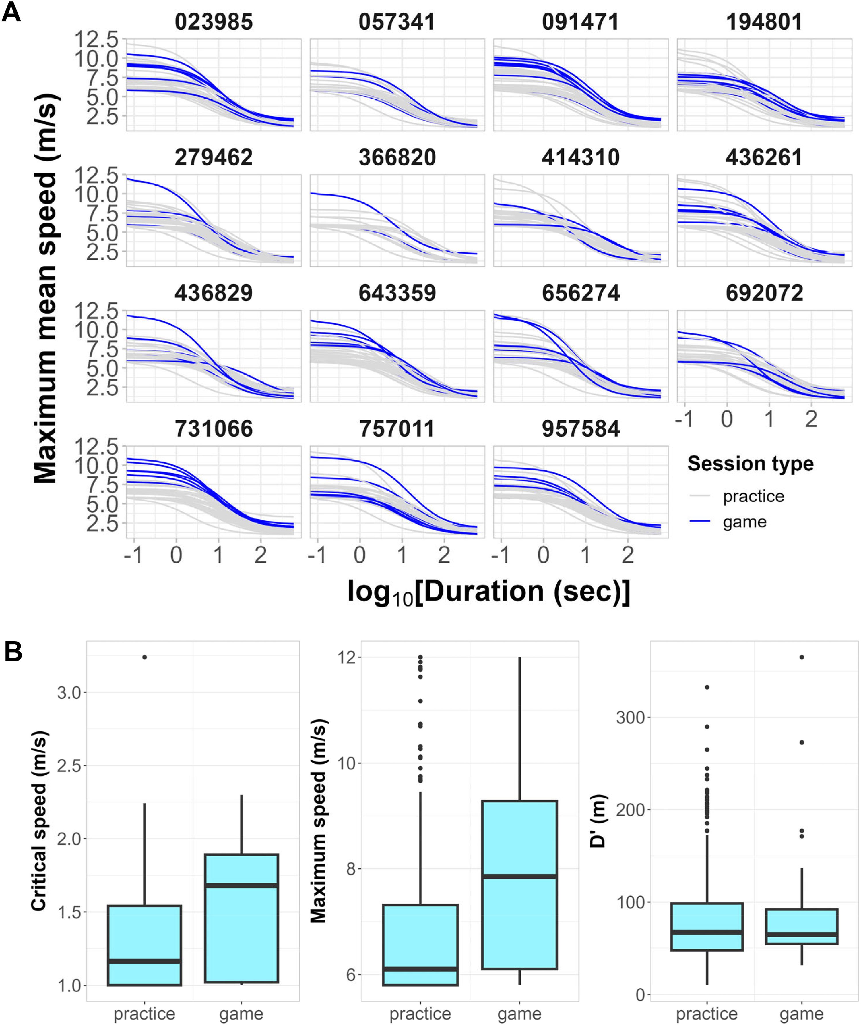
Critical speed models of high-resolution speed-duration profiles characterize the peak running demands for practices and games. (a) CS3 models of session-specific speed-duration profiles for each player, colored by practices (grey) and games (blue). (b) CS3 model parameter estimates (critical speed, maximum speed, D′) from the session-specific speed-duration profiles from practices and games. The critical speed and maximum speed were statistically higher for games compared to practices.

Discussion

In this study, we generated high-resolution speed-duration profiles derived from GPS data collected from collegiate soccer athletes, followed by testing the ability of CS models to fit the data and provide insights into the peak running demands in games and practices. Our study contributes novel methodology that can be incorporated into the repertoire of working sport scientists and coaches. Computationally, we developed publicly available R code that generates the high-resolution speed-duration profiles from raw GPS data. The software generates a maximal mean speed profile for a player from a dataset of approximately 38 sessions (practices, scrimmages, games) in less than 1 minute. This efficient computation can assist sport scientists to generate comprehensive speed-duration profiles in a time-efficient manner.

The speed-duration profiles generated by our methodology feature far higher resolution than previously studied profiles. Specifically, the profiles in this study featured approximately 6000 durations (from 2 to 600 seconds, in increments of 0.1 seconds) whereas those of previous studies featured six^25,26 or 21 durations.²⁰ The advantages and limitations of using lower and higher resolution sampling have yet to be systematically assessed. Intuitively, it stands to reason that using more of the available data ought to be more informative. Indeed, peak running demands for any duration can be straightforwardly extracted from the speed-duration profiles. Here, we extracted data on peak average velocities (also called “relative distances”) for 1, 3, 5, and 10-minute durations (Table 2), which are the durations that are most commonly reported in previous studies.⁶ The peak running demands of NCAA Division I male soccer players have yet to be characterized, such that our study adds to existing literature on the physical demands of men's NCAA Division I soccer (e.g. Refs. 33 –36). On the contrary, the high-resolution data present challenges for modeling. For example, data points that arise from the same segment of GPS data are not statistically independent. Standard parametric statistical inference techniques, for example computation of confidence intervals on the parameter estimates, typically assume statistical independence of the data, such that these techniques cannot be validly applied to estimates from single speed-duration profiles. By highlighting these issues and providing methodology for generating speed-duration profiles of various resolutions, our study provides a foundation for a future study of sampling issues with respect to speed-duration profiles.

Finally, we studied three models from the CS model family (CS2, CS3, OmSD), such that our study extends previous studies that employed only the CS2^25,26 model or empirical models.^17,18,20 The 5PL, CS3, and OmSD models markedly outperformed the CS2 model with respect to goodness of fit, as expected, and the three models exhibited minor statistically nonsignificant differences between them. We applied the CS2 model to speed-duration profiles featuring durations spanning 120 to 600 seconds, and we observed satisfactory goodness of fits (data not shown). This result was expected because this range of durations falls within the domain of validity for the CS2 model. Inspection of Figure 3 demonstrates that the CS3, OmSD, and 5PL models satisfactorily capture the trends of the speed-duration profiles for individual players, which suggests that they are useful for efficiently summarizing such data. Supplemental Tables S1 and S2 show the parameter values for each participant, for which we demonstrated that CS and D′ exhibited statistically significant variance between players. This result implies that the CS models could be used to profile and monitor individual players. We did not analyze contextual factors as part of this study, but it is likely that the differences between players arise due to both intrinsic (e.g. top-end speed, aerobic fitness) and extrinsic factors (e.g. position, being a starter or substitute, opponent quality, team tactics, etc.), as has been previously shown.^37,38 The effect of contextual variables on CS model parameters is a fruitful direction for future research.

Several limitations of our results were noted. First, lack of fit of the models was evident, with the residuals for all models exhibited systematic variation as a function of the fitted values (Supplemental Figure S2A). Second, the residuals were overdispersed and departed from normality (Supplemental Figure S2B). Finally, the data points are not statistically independent because clusters of data points come from the same segments (Figure 1(b) and (d); Supplemental Figure S2C). These issues might be addressable by (a) collecting data from more sessions, which would add more independent data points, and (b) employing statistical modeling approaches that account for nonnormality and statistically dependent residuals. Further truncation of the data is unlikely to resolve the independence issues.

We propose that the lack-of-fit was caused by issues both of data quality and by the assumptions and formulation of the models. The models were unable to capture two artifactual features of the data. First, the strongest discrepancies were noted at the highest speeds. For the fits of speed-duration profiles of the 0 to 600 seconds data, we noted for some players that the speeds for durations of 1 second and shorter were flat in profile, which occurred because we filtered speeds that exceeded 12 m s⁻¹. A potential resolution to this issue is to compute the velocities using a longer time span for the positional derivative calculation.³⁹ However, this approach can only be applied to velocities estimated from positional differentiation and not to velocities directly measured by Doppler shift,⁴⁰ which is the preferred velocity measure. Second, the intermittency of the efforts caused artifactual “bumps” in the speed-duration profiles (Figure 1(d)), which should theoretically be impossible to observe. Although not easily observed with our data, the models lack the ability to fit speeds at longer durations because they assume that the maximal sustainable speed asymptotes to CS as duration increases. The reality is that speed continually decreases as a function of duration, and the models cannot capture this trend without additional terms and parameters.²²

The intermittent nature of team-based field sports distinguishes them from endurance sports, for which power and speeds tend to be more constant. Indeed, soccer players tend to run at high intensity in bursts of short durations and perform low-intensity activities like walking and jogging for longer durations. The intermittency of soccer play led to CS estimates that are likely well below directly measured estimates for soccer players of the calibre studied. The observed critical speeds of approximately 2 m·s⁻¹ corresponds to a pace of 7.2 km h⁻¹. This pace is considered jogging by those who have previously studied male NCAA Division I soccer players.³⁶ In addition, NCAA Division I soccer players are considered well trained: they have $\dot{V} O_{2 \max}$ values of approximately 60 mL kg⁻¹ min⁻¹ and $\dot{V} O_{2}$ at ventilatory threshold of approximately 44 mL kg⁻¹ min⁻¹.⁴¹ The average running economies of moderately to highly trained runners predict a pace of 14 km h⁻¹ at a $\dot{V} O_{2}$ of approximately 45 mL kg⁻¹ min⁻¹.⁴² A similar pace should likewise be sustainable for these soccer players, such that 7 km h⁻¹ speed should be trivial for them to sustain, and thus well below their actual CS. Similar results were observed by Roecker et al.²⁰ but Lord et al. observed more reasonable CS estimates of approximately 4 m s^-1 in their studies.^25,26 Overall, it is questionable as to whether CS and D′ parameters estimated from CS models fit to speed-duration data will be equivalent to values estimated from formal testing. The lack of equivalence in values means that their physiological interpretation is not assured. Until the physiological interpretability of these parameters can be established, we propose renaming the CS parameter as the “asymptotic speed” (AS) and D′ as the curvature constant (CC) when employing CS models to speed-duration data obtained from intermittent sports.

In conclusion, our study contributes new methods and results pertaining to computing peak running demands in soccer athletes. Because of the complexity of high-resolution speed-duration profiles, we tested CS models for their ability to describe the profiles, finding that the CS3 and OmSD models provided satisfactory fits, and that the models could be used to distinguish between match and training demands. We observed several issues that could be addressed through future research: first, we observed manifestations of intermittent activity on the profiles, wherein some profiles featured “bumps” and CS values that are likely underestimated. Second, more sophisticated statistical methods that can accommodate non-independent data may be warranted to ensure valid statistical inferences from the profiles.

Practical applications

The results and methods from our study can be applied as follows. First, our study contributes publicly available R code to compute and model high-resolution speed-duration profiles from GPS data, which can be used by coaches and sport scientists to quantify peak running demands of field-based team sport athletes. The critspeed R package can be imported by users and its functions straightforwardly integrated into one's data analysis workflow. The code is open source and modifiable by users. The CS3, OmSD, and 5PL models effectively summarize the profiles and can be used to longitudinally monitor individual players, to compare positional demands, and to compare practice and game demands.

Coaches can use the data from our methods to plan and monitor training activities that mimic game demands, as has been widely recommended.^4,5,11,14 Training activities such as continuous runs at or near CS, high-intensity intervals, sprint intervals, repeat sprints, and small-sided games can all be used to improve the aerobic fitness and running endurance of soccer athletes.^43,44 Interval training permits strict control of work intensities in an individualized manner, but interval training does not challenge technical or tactical skills. In contrast, small-sided games seek to challenge fitness and technical and tactical skills, but their stochastic nature makes it challenging to control individual intensities and training loads. A mix of training activities could therefore be applied to challenge the various duration segments of the speed-duration profiles. We emphasize that not every training session should seek to match game demands, but perhaps the global speed-duration profiles for each player from one to two weeks’ worth of training should be largely similar to profiles from games. CS models of speed-duration profiles merit further study for this application.

Supplemental Material

sj-pdf-1-spo-10.1177_17479541241246951 - Supplemental material for Critical speed models of high-resolution speed-duration profiles describe peak running demands in soccer

Supplemental material, sj-pdf-1-spo-10.1177_17479541241246951 for Critical speed models of high-resolution speed-duration profiles describe peak running demands in soccer by Eliran Mizelman, Aaron Pearson, Dani Chu and David C Clarke in International Journal of Sports Science & Coaching

Supplemental Material

sj-csv-2-spo-10.1177_17479541241246951 - Supplemental material for Critical speed models of high-resolution speed-duration profiles describe peak running demands in soccer

Supplemental material, sj-csv-2-spo-10.1177_17479541241246951 for Critical speed models of high-resolution speed-duration profiles describe peak running demands in soccer by Eliran Mizelman, Aaron Pearson, Dani Chu and David C Clarke in International Journal of Sports Science & Coaching

Footnotes

Acknowledgements

The authors thank Sean Machak of Seattle University for coordinating the data collection and transfer, and Quynh Chi Nguyen, Zhi Yuh Ou Yang, and Angad Bajaj of Simon Fraser University for their contributions to coding the algorithms used in this study. This research was supported by funding from the SFU Key Big Data Initiative (Next Big Question grant to DCC and scholarship to EM) and by an Own The Podium Innovations 4 Gold grant to DCC.

Declaration of conflicting interests

The authors declared no potential conflicts of interest with respect to the research, authorship, and/or publication of this article.

Funding

The authors disclosed receipt of the following financial support for the research, authorship, and/or publication of this article: This work was supported by the SFU Key Big Data Initiative, Own The Podium (grant number Next Big Question grant, Innovation 4 Gold).

ORCID iD

David C Clarke

Supplemental material

Supplemental material for this article is available online.

References

Cummins

Orr

O’Connor

, et al. Global positioning systems (GPS) and microtechnology sensors in team sports: a systematic review. Sports Med 2013; 43: 1025–1042.

Hennessy

Jeffreys

. The current use of GPS, its potential, and limitations in soccer. Strength Cond J 2018; 40: 83–94.

Buchheit

Simpson

. Player-tracking technology: half-full or half-empty glass? Int J Sports Physiol Perform 2017; 12: S2–35–S2–41.

Wing

. Designing pre-season training programs using global positioning systems: a systematic approach. Strength Cond J 2019; 41: 27–38.

Weaving

Young

Riboli

, et al. The maximal intensity period: rationalising its use in team sports practice. Sport Med - Open 2022; 8: 128.

Rico-González

Oliveira

Vieira

LHP

, et al. Players’ performance during worst-case scenarios in professional soccer matches: a systematic review. Biol Sport 2022; 39: 695–713.

Fereday

Hills

Russell

, et al. A comparison of rolling averages versus discrete time epochs for assessing the worst-case scenario locomotor demands of professional soccer match-play. J Sci Med Sport 2020; 23: 764–769.

Oliva-Lozano

Martin-Fuentes

Fortes

, et al. Differences in worst-case scenarios calculated by fixed length and rolling average methods in professional soccer match-play. Biol Sport 2021; 38: 325–331.

Varley

Elias

Aughey

. Current match-analysis techniques’ underestimation of intense periods of high-velocity running. Int J Sports Physiol Perform 2012; 7: 183–185.

10.

Lacome

Simpson

Cholley

, et al.

Small-sided games in elite soccer: does one size fit all?

Int J Sports Physiol Perform 2018; 13: 568–576.

11.

McCall

Pruna

Van der Horst

, et al. Exercise-based strategies to prevent muscle injury in male elite footballers: an expert-led Delphi survey of 21 practitioners belonging to 18 teams from the Big-5 European leagues. Sport Med 2020; 50: 1667–1681.

12.

Johnston

Gabbett

Jenkins

. Applied sport science of rugby league. Sport Med 2014; 44: 1087–1100.

13.

Sydney

Wollin

Chapman

, et al.

Do conditioning focused various-sided training games prepare elite youth male soccer players for the demands of competition?

Biol Sport 2022; 39: 825–832.

14.

Riboli

Castagna

. Soccer-drill specificity in top-class male players with reference to peak match locomotor demands. J Sports Sci 2023; 41: 573–583.

15.

Riboli

Coratella

Rampichini

, et al. Area per player in small-sided games to replicate the external load and estimated physiological match demands in elite soccer players. PLoS One 2020; 15: e0229194.

16.

Riboli

Esposito

Coratella

. Small-sided games in elite football: practical solutions to replicate the 4-min match-derived maximal intensities. J Strength Cond Res 2023; 37: 366–374.

17.

Duthie

Thornton

Delaney

, et al. Running intensities in elite youth soccer by age and position. J Strength Cond Res 2018; 32: 2918–2924.

18.

Delaney

Thornton

Rowell

, et al. Modelling the decrement in running intensity within professional soccer players. Sci Med Footb 2018; 2: 86–92.

19.

Howe

Aughey

Hopkins

, et al. Modeling professional rugby union peak intensity–duration relationships using a power law. Int J Sports Physiol Perform 2022; 17: 780–786.

20.

Roecker

Mahler

Heyde

, et al. The relationship between movement speed and duration during soccer matches. PLoS One 2017; 12: e0181781.

21.

Quod

Martin

, et al. The power profile predicts road cycling MMP. Int J Sport Med 2010; 31: 397–401.

22.

Puchowicz

Baker

Clarke

. Development and field validation of an omni-domain power-duration model. J Sports Sci 2020; 38: 801–813.

23.

Housh

Cramer

Bull

, et al. The effect of mathematical modeling on critical velocity. Eur J Appl Physiol 2001; 84: 469–475.

24.

Poole

Burnley

Vanhatalo

, et al. Critical power: an important fatigue threshold in exercise physiology. Med Sci Sports Exerc 2016; 48: 2320–2334.

25.

Lord

Blazevich

Abbiss

, et al. Comparing maximal mean and critical speed and metabolic powers in elite and sub-elite soccer. Int J Sports Med 2020; 41: 219–226.

26.

Lord

Blazevich

Abbiss

, et al. Reliability and validity of maximal mean and critical speed and metabolic power in Australian youth soccer players. J Hum Kinet 2020; 73: 93–102.

27.

Menadue

. Validity and inter-unit reliability of 10 Hz GPS devices for assessing velocity in team-based field sports . Sport Performance Tracking technical report. 2019.

28.

R Core Team. R: a language and environment for statistical computing, https://www.r-project.org/ (2022).

29.

Morton

. A 3-parameter critical power model. Ergonomics 1996; 39: 611–619.

30.

Bertrand

Sakamoto

Ishiguro

, et al. Akaike information criterion statistics. J R Stat Soc Ser A (Statistics Soc) 1988; 151: 567.

31.

Akaike

. Information theory and an extension of the maximum likelihood principle. In: Parzen

Tanabe

Kitagawa

(eds) Selected papers of Hirotugu Akaike. Springer Series in Statistics. New York: Springer, 1998, pp.199–213.

32.

Schwarz

. Estimating the dimension of a model. Ann Stat 1978; 6: 461–464.

33.

Curtis

Huggins

Looney

, et al. Match demands of national collegiate athletic association division I men’s soccer. J Strength Cond Res 2018; 32: 2907–2917.

34.

Fields

Merigan

Gallo

, et al. External and internal load measures during preseason training in men collegiate soccer athletes. J Strength Cond Res 2021; 35: 2572–2578.

35.

Anderson

Adams

Martin

, et al. Examining internal and external physical workloads between training and competitive matches within collegiate division I men’s soccer. J Strength Cond Res 2021; 35: 3440–3447.

36.

Slater

Baker

Weltman

, et al. Activity monitoring in men’s college soccer: a single season longitudinal study. Res Sport Med 2018; 26: 178–190.

37.

Augusto

Brito

Aquino

, et al. Contextual variables affect peak running performance in elite soccer players: a brief report. Front Sport Act Living 2022; 4: 966146.

38.

Curtis

Huggins

Benjamin

, et al. Contextual factors influencing external and internal training loads in collegiate men’s soccer. J Strength Cond Res 2020; 34: 374–381.

39.

Swartz

. The calculation of player speed from tracking data. Int J Sports Sci Coach 2023; 18: 516–522.

40.

Malone

Lovell

Varley

, et al. Unpacking the black box: applications and considerations for using GPS devices in sport. Int J Sports Physiol Perform 2017; 12: S2–18–S2–26.

41.

Watson

Brindle

Brickson

, et al. Preseason aerobic capacity is an independent predictor of in-season injury in collegiate soccer players. Clin J Sport Med 2017; 27: 302–307.

42.

Barnes

Kilding

. Running economy: measurement, norms, and determining factors. Sport Med 2015; 1: 1–15.

43.

Iaia

Ermanno

Bangsbo

. High-intensity training in football. Int J Sports Physiol Perform 2009; 4: 291–306.

44.

Morgans

Orme

Anderson

, et al. Principles and practices of training for soccer. J Sport Health Sci 2014; 3: 251–257.

Supplementary Material

Please find the following supplemental material available below.

For Open Access articles published under a Creative Commons License, all supplemental material carries the same license as the article it is associated with.

For non-Open Access articles published, all supplemental material carries a non-exclusive license, and permission requests for re-use of supplemental material or any part of supplemental material shall be sent directly to the copyright owner as specified in the copyright notice associated with the article.

0.00 MB

3.86 MB

0.80 MB