Bayesian approaches for critical velocity modelling of data from intermittent efforts

Abstract

In sports science, critical power and related critical velocity models have been widely investigated, and are being increasingly applied to field-based team sports. A challenge associated with these models is that laboratory experiments that yield accurate measurements of maximal sustainable velocity are expensive. Alternatively, inexpensive field data (from training and matches) are being used to fit such models. However, the intermittent nature of efforts in field-based sports implies that the dependent variable concerning maximum sustainable velocity is reliably calibrated only for short time durations. This paper develops methods where field data based on short time durations is combined with prior knowledge to fit the three-parameter critical velocity model. This is accomplished in a Bayesian framework for which Markov chain methods are required for model fitting and inference.

Introduction

Critical power and critical velocity models are widely researched models in sports science. Critical power models investigate the relationship between the maximum intensity (power) that an athlete can sustain in a given time duration versus the time duration. Critical velocity models investigate the relationship between the maximum speed that an athlete can sustain in a given time duration versus the time duration. Knowledge of critical power and critical velocity relationships is useful for optimizing athletic training programs and pacing strategies. Critical velocity and critical power models have been studied across various sports including cycling, running, rowing and swimming. ¹ Critical power models have also been identified as potential tools in the detection of doping in sport ² and have been extended to whole-body exercise. ³

The two-parameter critical power model was first introduced by Monod and Scherrer ⁴ who referred to it as the CP model. The CP model has since been utilized in the context of critical velocity where it is known as the CV-2 model. The original CP model has been generalized in various directions to improve model fit. For example, Jones and Vanhatalo ⁵ consider activities where exercise intensity varies. In these activities, CP models have been introduced that allow for the reconstitution of power during lower intensity periods. A limitation of the CV-2 model (or any CV model with an asymptote) is that it yields an infinite maximal sustainable velocity as the time duration $t\to 0$ . Another limitation of the CV-2 model is that it implies that athletes can maintain a maximal sustainable velocity for infinite periods of time. Our focus will mainly concern the CV-3 model proposed by Morton ⁶ which provides a more realistic relationship between maximum sustainable speed and time duration.

In this work, we are explicit about the statistical assumptions that arise in the context of critical velocity models. In particular, we explore the types of data that arise and how this impacts the reliability of calibration. Statistical independence and correlation are investigated, as well as the distributional assumptions associated with measurement error. All of these topics impact the estimation of parameters in critical velocity models. Incorrect model assumptions can lead to biased parameter estimates. Statistical insight has proven valuable to problems arising in sports science and sports analytics. ⁷

Careful consideration of the features and limitations of critical velocity data leads to modelling opportunities. A primary contribution of this paper is the development of the CV-3 model in a Bayesian setting. In this case, the Bayesian framework is applied by synthesizing prior knowledge from laboratory settings with ‘inexpensive’ data obtained from training sessions. By inexpensive, we mean that the data are conveniently obtained from athletes during training sessions through the inconspicuous use of wearable devices. Because field-based sports tend to feature intermittent efforts (e.g., repeated sprints interspersed with walking and jogging), it is recognized that maximal speeds when extracted from training data are only reliable for short time durations. Consequently, in our proposed method, only short time duration data are utilized, and the information shortfall is supplemented by prior information gathered from gold-standard laboratory-based testing. Ideally, such data would be obtained from the same group of athletes; however, in the absence of such data, data collected from an independent sample of athletes can be used instead.

Therefore, the main focus of the paper concerns situations where no laboratory measurements are available and critical velocity parameters for an athlete cannot be estimated. Yet, by introducing unintrusive training data, reliable critical velocity parameter estimates may be obtained. Our careful consideration of model assumptions (including the correlations between observations) is taken into account. Another contribution of the paper is the development of a framework to study the adequacy of the ‘maximal moving average’ formula ⁸ as an estimator of maximal sustainable velocity. In Appendix A, we describe how this problem can be addressed via simulation studies where the design of the training session impacts the adequacy of the estimation procedure. We confirm the intuition that the maximal moving average formula does not work well for prolonged durations.

In a sports science application, Peng et al. ⁹ have proposed Bayesian methods and elicited priors in the context of the impulse-response model. Clarke and Skiba ¹⁰ emphasize the pedagogical importance of performance modelling in exercise physiology; discussion is provided in the context of critical power models and the impulse-response model.

In the ‘Data in critical velocity models’ section, we discuss how data are typically collected in the context of fitting critical velocity models. We specifically highlight the pitfalls of measuring maximal sustainable velocities for prolonged durations using wearable devices. In the ‘Model development’ section, the CV-2 and CV-3 models are presented from a statistical perspective. The assumptions related to the models are clearly specified, and the impact and relevance of these assumptions are discussed. In ‘A Bayesian version of the CV-3 model’ section, Bayesian formulations of the CV-3 model are presented. The motivation is that prior knowledge based on laboratory testing can be combined with field data to provide adequate estimates of the CV-3 parameters. Computational and inferential aspects are discussed. The methods are illustrated via an example in the ‘Example’ section. The ‘Discussion’ section provides a short discussion and outlines future research opportunities.

Data in critical velocity models

Critical velocity data are collected in various formats. Gold standard data which are considered the most reliable measurements are obtained in laboratory settings. Such data are naturally time consuming and expensive. And of course, the reliability of such data is dependent on athletes providing full effort.

Laboratory data are collected using various schemes including treadmill tests and shuttle run tests. For example, in a shuttle run test, two physical endpoints are constructed $m$ metres apart, and an athlete is requested to run continuously and alternatively, from one endpoint to the other within $s$ seconds. The athlete is asked to continue the exercise as long as possible, and upon exhaustion, completes $x$ traversals (i.e. from one end to the other). The response variable $y_t=m/s$ is the maximum speed (measured in metres per second) that the athlete sustains during the time duration $t=xs$ s. For example, suppose that the endpoints are spaced $m=35$ m apart. Suppose further that the athlete runs between endpoints in $s=5.0$ s, and accomplishes this $x=10$ times prior to collapsing. Then the athlete will have run for a duration of $t=xs=10(5.0)=50$ s, maintaining a maximal sustainable velocity of $y_t=y_{50}=m/s=35/5.0=7.0$ m/s.

Due to fatigue, it is intuitive that $y_t$ ought to be modelled as a decreasing function of $t$ . It is also clear that an athlete cannot be asked to repeat the exercise for different values of $t$ without recovery periods. Therefore, the collection of $y_t$ for different values of $t$ may take place over multiple sessions. This contributes to the expense of gold standard data collection. Laboratory testing also distracts from training, and may not be welcomed by athletes and coaches.

A less expensive data collection method involves the use of wearable sensing systems during training and matches. Prominent sensing systems are based on GPS (global positioning system) technology for which there are various commercial providers. For a given athlete, a ‘wearable’ sensing device provides positioning data from which velocities are obtained. Typically, GPS sensors capture data at a sample rate of 10–20  Hz. Let

$$v_1,v_2,\dots ,v_N$$

(1)

denote the instantaneous velocity data during a training session where the observations are dependent. For illustration, and without loss of generality, $v_i$ in Equation (1) refers to the instantaneous speed of the athlete in metres per second at second $i$ of training, and the training session consists of $N$ seconds. For example, in a 1.5-h training session, $N=5400$ . Therefore, sensing data may be considered ‘big data’, and are inexpensive in the sense that athletes simply carry out normal activities. Wearable devices can provide much more information in addition to instantaneous speed measurements. For example, location data, acceleration data and physiological measurements may also be recorded through wearables. A review of various wearable devices including an assessment of measurement accuracy is given by Lutz et al. ¹¹ Since measurement errors may be present in the recording of instantaneous speeds, pre-processing is recommended in which a maximum velocity threshold is determined for the raw data in Equation (1). The threshold may be set by looking at the data, identifying outliers and assessing what may be reasonable upper bound for a given athlete. Pre-processing techniques for GPS data are discussed in detail by Abbruzzo, Ferrante and de Cantis. ¹²

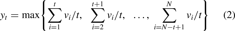
In the context of critical velocity models, an immediate question concerns the relationship between the field measurements $v_i$ in Equation (1) to maximal sustainable velocities. A common approach defines a response variable $y_t$ referred to as the maximal moving-average ⁸ as

$$y_t=max\{\sum _{i=1}^t{v}_i/t,\sum _{i=2}^{t+1}{v}_i/t,\dots ,\sum _{i=N-t+1}^N{v}_i/t\}$$

(2)

where again for illustration, $t=1,\dots ,N$ is the time duration measured in seconds. Each component in Equation (2) is an average speed taken over a period of $t$ seconds. What is not entirely clear is why $y_t$ in Equation (2) is thought to be a good approximation of maximal sustainable speed for time duration $t$ . For large values of $t$ , one could realistically imagine an athlete slowing down and taking a rest for portions of every component interval; in this case $y_t$ in Equation (2) underestimates maximal sustainable velocity. On the other hand, for small values of $t$ , one might expect that there is some period of time duration $t$ where an athlete is running at a nearly constant speed, nearly as fast as possible, and the average over the period reasonably captures maximal sustainable velocity. For example, coaches could design sessions with specific drills that are expected to generate maximal sustainable velocities. This provides the motivation for the proposed methods that follow. Specifically, we will assume that training (field) data $y_t$ in Equation (2) collected through wearable devices provides reliable information on maximal sustainable speeds for short time durations $t$ . Again, we emphasize that, unlike laboratory data, field data are easy to collect.

In Appendix A, we use point processes and simulation studies to explore the adequacy of the maximal moving average Equation (2) as an approximation to maximal sustainable velocity. This appears to be the first investigation of the adequacy of this widely used approximation. As anticipated, the formula is not a good approximation for prolonged durations. An additional message from Appendix A is that the adequacy of the maximal moving average formula deteriorates with activities (matches or training) having frequent rest intervals.

Model development

Since the CV-2 model ⁴ provides the foundation for all critical power and critical velocity models, we begin by examining modelling issues with respect to this simple model. We then transition to the CV-3 model ⁶ which provides a more realistic description of the relationship between maximum sustainable velocity and time duration. The CV-3 model is examined in ‘A Bayesian version of the CV-3 model’ section, where short-duration field data are supplemented with prior knowledge under the Bayesian framework.

The CV-2 model

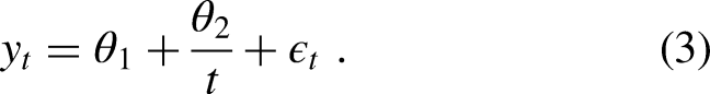
The simplest of the critical velocity models is a decreasing rational function referred to as the CV-2 model. Using the notation presented in the ‘Data in critical velocity models’ section, we write the CV-2 model for a particular athlete as

$$y_t={\theta }_1+\frac{{\theta }_2}{t}+{ϵ}_t.$$

(3)

Using conventional statistical notation, the two unknown parameters in Equation (3) are the quantities of interest and are expressed using the Greek symbols ${\theta }_1>0$ and ${\theta }_2>0$ , respectively. The variable $y_t$ is the observed response, the time duration $t$ is the observed covariate, and the unobserved ${ϵ}_t$ term denotes random error. For probabilistic assessment of the model, distributional assumptions concerning ${ϵ}_t$ need to be introduced. In the above formulation, $t$ is fixed (i.e. not random) and $y_t$ inherits randomness from the error term. Burnley and Jones ¹³ provide a detailed discussion of the physiological aspects of the model (3). Using laboratory data, Patoz et al. ¹⁴ consider inferential aspects associated with the CV-2 model. In particular, they investigate the bias associated with various weighted least squares fitting procedures.

In the sports science literature, ${\theta }_1$ is typically referred to as critical velocity and is written as $CV$ . In the critical power setting, ${\theta }_1$ is referred to as critical power and is written as $CP$ . Mathematically, ${\theta }_1$ is the value of the limiting asymptote corresponding to large time durations $t$ . Immediately, we see a theoretical failing in the CV-2 model (3), since it is physiologically impossible for athletes to sustain a threshold of performance for unbounded periods of time. For moderate time durations, the critical velocity model may be both practical and adequate.

In the sports science literature, the parameter ${\theta }_2$ is typically written as $D^{\prime }$ in the critical velocity setting and $W^{\prime }$ in the critical power setting. In the critical velocity setting, the expected value of ${ϵ}_t$ is zero, i.e. $\mathrm{E}({ϵ}_{\mathrm{t}})=0$ , and we can therefore express the parameter ${\theta }_2$ as a product of time and speed via ${\theta }_2=t(\mathrm{E}(y_t)-{\theta }_1)$ . It follows that ${\theta }_2$ has an interpretation as the expected distance that can be travelled in excess of the distance travelled at critical velocity for any time duration $t$ . We also note that in the sports science literature, the recognition and the assumptions concerning ${ϵ}_t$ are generally not made explicit. Typically, the ${ϵ}_t$ are assumed to be independent, normally distributed with mean zero and common variance. However, as previously discussed, with data arising from training sessions, there is dependence on the response variable (2). Such assumptions are important as they impact statistical inference involving the parameters ${\theta }_1$ and ${\theta }_2$ .

An immediate limitation of the fitted CV-2 model ${\hat{y}}_t={\hat{\theta }}_t+{\hat{\theta }}_2/t$ is that the estimated instantaneous maximal speed of the athlete $\underset{t\to 0}{lim}{\hat{y}}_t$ is infinite. Importantly, this limitation is not just a mathematical curiosity corresponding to $t=0$ . If we take a typical estimate $({\hat{\theta }}_1,{\hat{\theta }}_2)=$ (4 m/s, 200 m) obtained from Dicks et al., ¹⁵ we observe that even for time durations as large as $t=20$ seconds, the estimated sustainable velocity for the athlete would be 14.0  m/s corresponding to an impossibly fast 50.4  km/h.

The CV-3 model

Again, we prefer to use conventional notation for statistical models where the response variable is on the left hand side of the equation and model parameters are denoted using Greek symbols. Doing so and re-parametrizing, Morton’s three-parameter CV-3 model ⁶ can be expressed as

$$y_t={\theta }_1+{\theta }_2/(t+{\theta }_3)+{ϵ}_t.$$

(4)

The parametrization (4) provides a simplification of what one typically sees in the sports science literature and aids in the interpretation of parameters. For example, the ${\theta }_3$ parameter provides a leftward shift of the CV-2 model (3) by ${\theta }_3$ units in the variable $t$ . Moreover, as ${\theta }_3\to 0$ , the CV-3 model reduces to the CV-2 model. In this parametrization, ${\theta }_1>0$ maintains the same interpretation as in the CV-2 model and ${\theta }_2$ determines the curvature. Although the CV-3 model (4) is not linear in the parameters ${\theta }_1$ , ${\theta }_2$ and ${\theta }_3$ and consequently do not benefit from linear model theory, the parametrization has various appealing properties. First, as logic involving maximal sustainable speeds would suggest, it can be shown that ${\hat{y}}_t={\hat{\theta }}_1+{\hat{\theta }}_2/(t+{\hat{\theta }}_3)$ is a decreasing function of $t$ . Second, the instantaneous maximal speed ${\hat{y}}_0={\hat{\theta }}_1+{\hat{\theta }}_2/{\hat{\theta }}_3$ is necessarily finite, and unlike the CV-2 model, the CV-3 model provides sensible maximal sustainable speeds for short time durations $t$ . In the parametrization specified in equation (4), we impose the restrictions ${\theta }_1>0$ , ${\theta }_2>0$ and ${\theta }_3>0$ .

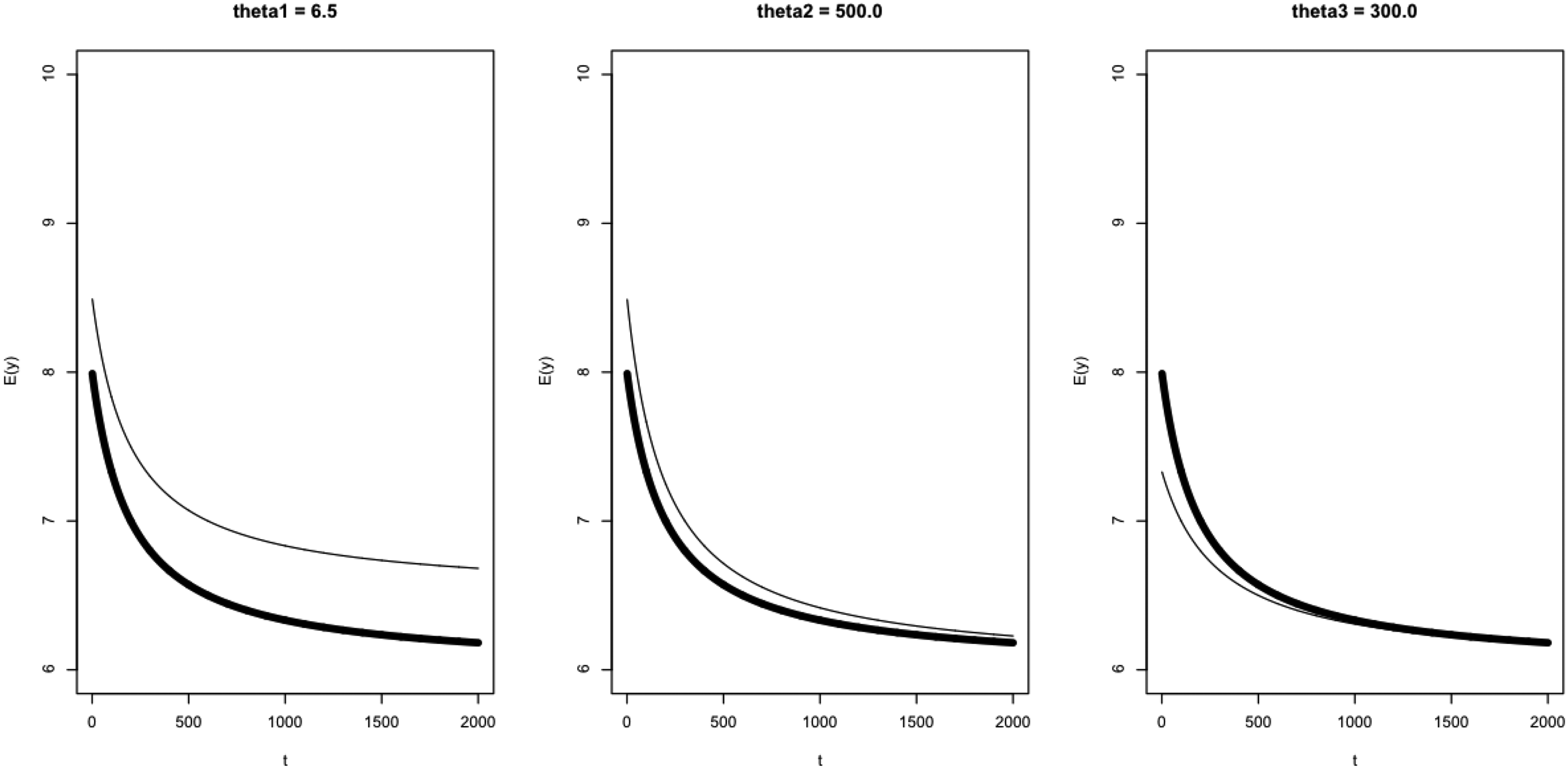
In Figure 1, we demonstrate the role of the parameters ${\theta }_1$ , ${\theta }_2$ and ${\theta }_3$ in Equation (4) by plotting various CV-3 models. We see that ${\theta }_1$ alters the vertical displacement, whereas ${\theta }_2$ and ${\theta }_3$ impact the curvature.

Figure 1.

Plots of the expected CV-3 model given by $\mathrm{E}(y_t)={\theta }_1+{\theta }_2/(t+{\theta }_3)$ . The bold line corresponds to realistic settings of the parameters, ${\theta }_1=6.0$ , ${\theta }_2=400.0$ and ${\theta }_3=200.0$ . The thin lines correspond to a change in a single parameter as indicated by the main captions.

A Bayesian version of the CV-3 model

In Bayesian frameworks, classical statistical models are augmented with prior knowledge of parameters through the use of prior distributions. The synthesis of the two components results in a posterior distribution which gives the complete probabilistic description of the parameters.

Initial model

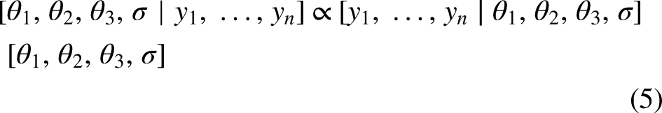
Let $[A\mid B]$ generically denote the density function corresponding to $A$ given $B$ . Then based on Equation (4), and the introduction of the parameter $\sigma$ which characterizes variability in the data, the Bayesian paradigm expresses the posterior density of $({\theta }_1,{\theta }_2,{\theta }_3,\sigma )$ as

$$\begin{array}{rl}[& {\theta }_1,{\theta }_2,{\theta }_3,\sigma |y_1,\dots ,y_n]\propto [y_1,\dots ,y_n\mid {\theta }_1,{\theta }_2,{\theta }_3,\sigma ]\\ & [{\theta }_1,{\theta }_2,{\theta }_3,\sigma ]\end{array}$$

(5)

where $y_1,\dots ,y_n$ are field data as specified in Equation (2). Note that $n$ is the number of maximal velocity observations that have been included in the model. The variable $n$ is chosen sufficiently small such that $y_t$ accurately measures maximal sustainable velocity for time duration $t$ , $t=1,\dots ,n$ . The term $[y_1,\dots ,y_n\mid {\theta }_1,{\theta }_2,{\theta }_3,\sigma ]$ is referred to as the likelihood, where the precise form of the likelihood is determined by the distributional assumptions assigned to the ${ϵ}_t$ terms in Equation (4). The term $[{\theta }_1,{\theta }_2,{\theta }_3,\sigma ]$ specifies the prior distribution concerning the parameters ${\theta }_1$ , ${\theta }_2$ , ${\theta }_3$ and $\sigma$ .

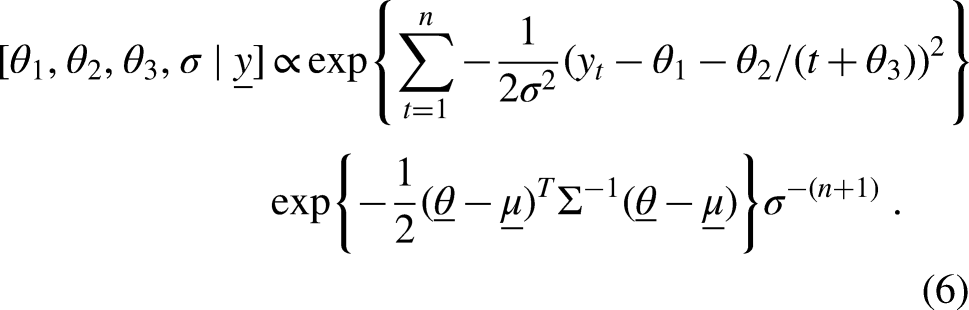
We begin with some strong but standard assumptions involving the initial model. First, we assume that the error terms ${ϵ}_1,\dots ,{ϵ}_n$ are independent with ${ϵ}_t\sim \mathrm{Normal}[0,{\sigma }^2]$ . The consequence of the distributional assumption is that the field data $\underset{\_}{y}=(y_1,\dots ,y_n{)}^T$ are conditionally independent and that $y_t\sim \mathrm{Normal}[{\theta }_1+{\theta }_2/(t+{\theta }_3),{\sigma }^2]$ . We further assume that $\underset{\_}{\theta }=({\theta }_1,{\theta }_2,{\theta }_3{)}^T$ is statistically independent of $\sigma$ , where we assign Jeffreys reference prior $[\sigma ]\propto 1/\sigma$ . We assign the multivariate normal distribution $\underset{\_}{\theta }\sim {\mathrm{Normal}}_3[\underset{\_}{\mu },\mathrm{\Sigma }]$ where $\underset{\_}{\mu }=({\mu }_1$ , ${\mu }_2,{\mu }_3{)}^T$ and $\mathrm{\Sigma }$ are specified hyperparameters. Instead, it would also be possible to consider a truncated multivariate normal distribution where the constraints ${\theta }_1>0$ , ${\theta }_2>0$ and ${\theta }_3>0$ are imposed. Under these assumptions, the posterior density (5) reduces to

$$\begin{array}{rl}[{\theta }_1,{\theta }_2,{\theta }_3,\sigma |\underset{\_}{y}]& \propto \exp \{\sum _{t=1}^n-\frac{1}{2{\sigma }^2}(y_t-{\theta }_1-{\theta }_2/(t+{\theta }_3){)}^2\}\\ & \exp \{-\frac{1}{2}(\underset{\_}{\theta }-\underset{\_}{\mu }{)}^T{\mathrm{\Sigma }}^{-1}(\underset{\_}{\theta }-\underset{\_}{\mu })\}{\sigma }^{-(n+1)}.\end{array}$$

(6)

There is a remaining detail that needs to be overcome in the specification of the posterior density (6). That is, we require the specification of the mean vector $\underset{\_}{\mu }$ and the variance-covariance matrix $\mathrm{\Sigma }$ , which convey prior opinion concerning the parameter vector $\theta$ . Imagine that we have estimates $({\hat{\theta }}_{11},{\hat{\theta }}_{12},{\hat{\theta }}_{13})$ , $({\hat{\theta }}_{21},{\hat{\theta }}_{22},{\hat{\theta }}_{23})$ , …, $({\hat{\theta }}_{m1},{\hat{\theta }}_{m2},{\hat{\theta }}_{m3})$ for $m$ athletes whose estimates were obtained from gold standard laboratory testing. Recall again that such estimates are expensive but are thought to be reliable. It would be sensible if the athlete in question resembled this population of athletes. For example, if the athlete was a high-level rower, you would prefer laboratory data involving rowers of the same sex, comparable competitive levels and similar ages. In this case, all that one needs to do is average the estimates to obtain $\underset{\_}{\mu }$ , i.e. ${\mu }_j=(1/m)\sum _{i=1}^m{\hat{\theta }}_{ij}$ , for $j=1,2,3$ . Similarly, $\mathrm{\Sigma }=({\sigma }_{ij})$ is specified by calculating sample variances and sample covariances; ${\sigma }_{ij}=(1/m)\sum _{k=1}^m({\hat{\theta }}_{ki}-{\mu }_i)({\hat{\theta }}_{kj}-{\mu }_j)$ . Of course, other approaches for the specification of the hyperparameters $\underset{\_}{\mu }$ and $\mathrm{\Sigma }$ are possible.

A more complex model

We now weaken some of the assumptions introduced in the initial model.

We first recognize that the observations $y_1,\dots ,y_n$ obtained through training sessions are not likely to be conditionally independent. Referring to Equation (2), it is likely that the interval $v_k,v_{k+1},\dots ,v_{k+t-1}$ which yields $y_t$ overlaps with the interval which yields $y_{t-1}$ . Consequently, the field data $y_t$ and $y_{t+\mathrm{\Delta }}$ are more likely to be similar when the time difference $\mathrm{\Delta }$ is small.

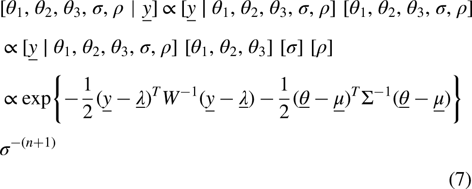
This insight may be modelled by introducing greater structure on the likelihood term in Equation (5). Specifically, we model $[y_1,\dots ,y_n\mid {\theta }_1,{\theta }_2,{\theta }_3]$ as a multivariate ${\mathrm{Normal}}_n[\underset{\_}{\lambda },W]$ density where ${\lambda }_t={\theta }_1+{\theta }_2/(t+{\theta }_3)$ and $W$ is defined as a first order autoregressive covariance matrix whose $(i,j)$ th element is ${\sigma }^2{\rho }^{\mid i-j\mid }$ and the correlation between the $i$ th term $y_i$ and the $j$ th term $y_j$ is ${\rho }^{\mid i-j\mid }$ . We refer to $\rho \in (0,1)$ as the correlation parameter. The consequence is that field data $y_t$ and $y_{t+\mathrm{\Delta }}$ are more positively correlated when the time difference $\mathrm{\Delta }$ is small. The proposed approach has the benefit of ‘smoothing’ the data $y_1,\dots ,y_n$ . This idea has been used in the analysis of substitution times in soccer. ¹⁶ The additional parameter $\rho$ is assumed independent of the remaining parameters and we assign $\rho \sim \mathrm{Uniform}(0,1)$ .

The net effect of the additional modelling is that the posterior now takes the form

$$\begin{array}{rl}& [{\theta }_1,{\theta }_2,{\theta }_3,\sigma ,\rho |\underset{\_}{y}]\propto [\underset{\_}{y}\mid {\theta }_1,{\theta }_2,{\theta }_3,\sigma ,\rho ][{\theta }_1,{\theta }_2,{\theta }_3,\sigma ,\rho ]\\ & \propto [\underset{\_}{y}\mid {\theta }_1,{\theta }_2,{\theta }_3,\sigma ,\rho ][{\theta }_1,{\theta }_2,{\theta }_3][\sigma ][\rho ]\\ & \propto \exp \{-\frac{1}{2}(\underset{\_}{y}-\underset{\_}{\lambda }{)}^T{W}^{-1}(\underset{\_}{y}-\underset{\_}{\lambda })-\frac{1}{2}(\underset{\_}{\theta }-\underset{\_}{\mu }{)}^T{\mathrm{\Sigma }}^{-1}(\underset{\_}{\theta }-\underset{\_}{\mu })\}\\ & {\sigma }^{-(n+1)}\end{array}$$

(7)

where we note that $\underset{\_}{\lambda }$ is a function of $({\theta }_1,{\theta }_2,{\theta }_3)$ and the matrix $W$ is a function of $(\sigma ,\rho )$ .

Computation and Inference

Based on the synthesis of data and prior knowledge, the posterior distributions (6) and (7) fully describe the uncertainty in the parameters. However, as written, these densities are complex, are not recognizable as familiar parametric distributions and are not readily interpretable. Therefore, it would be instructive to obtain posterior summaries of the parameters of interest ${\theta }_1$ , ${\theta }_2$ and ${\theta }_3$ . Examples of posterior summaries are posterior means and posterior standard deviations which themselves are not analytically tractable quantities. The remedy is to generate the parameters from the posterior distributions using Markov chain Monte Carlo (MCMC) methods.

Here, MCMC is carried out using JAGS software. ¹⁷ A feature of JAGS is that the experimenter does not have to derive the full conditional distributions required to implement Gibbs sampling (a basic version of MCMC). Rather, the experimenter needs only to provide the data, and specify both the sampling and prior distributions. With this information, MCMC variate generation is carried out by JAGS in the background. Upon practical convergence of the MCMC algorithm, the experimenter is provided with posterior samples from the posterior distribution. The samples are then used for inferential purposes. For example, a user may average the samples of a parameter to approximate its posterior mean. It is also possible to create density plots based on the samples to approximate posterior density functions.

Example

It is good to provide an overview of our problem. Imagine an athlete for whom we want estimates of critical velocity parameters, but there is no laboratory data. Perhaps the best that can be done is to simply reason that their parameters are similar to the average values of comparable athletes. Our belief is that we can do better than that. We can take data from unintrusive training sessions and use the reliable short duration measurements to modify the average values. The method for doing this is not arbitrary – it is the well-established Bayesian approach.

The test case that we consider is based on field data arising as in Equation (1) and converted to $y_t$ measurements as specified in Equation (2). In this case, the field data corresponds to a single 90 min soccer match by an anonymous forward in the Chinese Super League (CSL) during the 2019 season. The data were acquired via cameras and optical recognition software by the provider TRACAB.

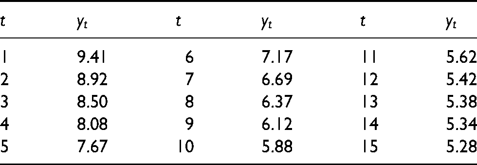
The measurements $y_t$ are recorded in Table 1 and correspond to time durations $t=1,2,\dots ,15$ s. In soccer matches, players do not typically run full out for 15 consecutive seconds. The sport involves frequent starts, changes of direction, and periods of rest. Therefore, we expect the measurements in Table 1 to be less reliable for larger values of $t$ . Note that $y_1=9.41$   m/s nearly represents maximal speed and corresponds to 33.9  km/h. For reference, the maximum speed attained by Usain Bolt over a 20-m section at the IAAF World Challenge in Zagreb 2011 was 43.7  km/h. ¹⁸ We utilize short time durations $y_1,\dots ,y_5$ as our measurements in fitting CV-3 models. Note that the $y_t$ are decreasing, although according to the construction in Equation (2), this does not mathematically need to be the case. Therefore, with limited data (i.e. $n=5$ data points), we are attempting to fit useful 3-parameter models. What makes this possible is the Bayesian construction where we supplement field data with informative prior knowledge. And, we repeat, a main feature of the approach is that the field data are obtained inexpensively.

Table 1.

Values $y_t$ from Equation (2) measured in m/s for a forward during a CSL match.

$t$	$y_t$	$t$	$y_t$	$t$	$y_t$
1	9.41	6	7.17	11	5.62
2	8.92	7	6.69	12	5.42
3	8.50	8	6.37	13	5.38
4	8.08	9	6.12	14	5.34
5	7.67	10	5.88	15	5.28

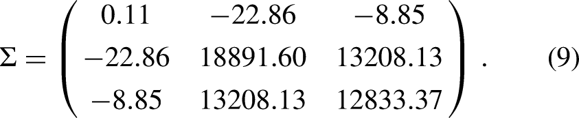
The next step involved in the implementation of the Bayesian analyses requires the specification of the hyperparameters $\underset{\_}{\mu }$ and $\mathrm{\Sigma }$ which are common to both models (6) and (7). Referring to Morton ⁶ , we can reparametrize the fitted parameters corresponding to the six long distance runners in Table 8 (middle three columns). Then following the discussion at the end the ‘Initial model’ section, we obtain hyperparameters

$$({\mu }_1,{\mu }_2,{\mu }_3)=(5.82,396.00,198.21{)}^T$$

(8)

and

$$\begin{array}{r}\mathrm{\Sigma }=\left(\begin{array}{ccc}0.11& -22.86& -8.85\\ -22.86& 18891.60& 13208.13\\ -8.85& 13208.13& 12833.37\end{array}\right).\end{array}$$

(9)

From Equation (8), the prior estimate of critical velocity ${\mu }_1=5.82$   m/s corresponds to 21.0  km/h. This value likely overestimates the player’s critical velocity and highlights the importance of having good prior information. Using Equation (8), we also obtain the prior estimate ${\mu }_1+{\mu }_2/{\mu }_3=7.81$   m/s of instantaneous velocity which corresponds to 28.1  km/h. Using the relationship between covariances and correlation, we calculate from Equation (9) that there are meaningful prior correlations between the parameters. Specifically, we obtain $\mathrm{Corr}({\theta }_1,{\theta }_2)=-0.50$ , $\mathrm{Corr}({\theta }_1,{\theta }_3)=-0.24$ and $\mathrm{Corr}({\theta }_2,{\theta }_3)=0.85$ . Recognizing that reliable prior information is important and that the long distance runners studied by Morton ⁶ may differ from soccer players, we introduce a conservative procedure and inflate $\mathrm{\Sigma }$ in Equation (9) using $k\mathrm{\Sigma }$ where $k>0$ is a tuning parameter. An inflated value of $\mathrm{\Sigma }$ introduces greater variability in the prior distribution and consequently puts more inferential emphasis on the data. For illustration, we set $k=1.5$ .

With observations $y_1,\dots ,y_5$ from Table 1 and prior knowledge as expressed in Equations (8) and (9), we fit three models; the classical model $y_t\sim \mathrm{Normal}[{\theta }_1+{\theta }_2/(t+{\theta }_3),{\sigma }^2]$ using maximum likelihood estimation, the initial Bayesian model (6) and the enhanced Bayesian model (7). For the latter two models, computation was carried out in JAGS based on 20,000 iterations where practical convergence of the chain was quickly achieved. From the MCMC output, 5000 iterations were discarded as burn-in, and 15,000 iterations were used for inference. The MCMC iterations required less than 1.0 s of computation on a laptop computer. Note that a feature of simulation output is that it facilitates estimation of functionals. For example, the instantaneous velocity $\mathrm{MaxV}={\theta }_1+{\theta }_2/{\theta }_3$ is a functional of interest as it is a function of the parameters ${\theta }_1$ , ${\theta }_2$ and ${\theta }_3$ . The fact that $\mathrm{MaxV}$ is relatively complex and does not have an apparent closed-form estimator is unimportant. In an MCMC setting, we can readily estimate the instantaneous velocity $\mathrm{MaxV}$ via the generated output of the primary parameters ${\theta }_1$ , ${\theta }_2$ and ${\theta }_3$ .

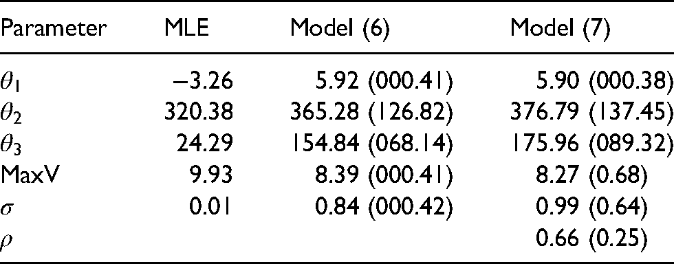
The estimated parameters are provided in Table 2. From Table 2, we immediately observe that maximum likelihood estimation (MLE) based on only five observations provides unrealistic CV-3 estimates. For example, the estimate of ${\theta }_1$ is negative. Therefore, it is apparent that field data on its own with only five data points cannot be used to estimate CV-3 parameters. It seems that auxiliary information is necessary for this application. Accordingly, we supplement the field data with prior knowledge in a Bayesian framework leading to the estimates corresponding to Models (6) and (7). An important observation is the field data impact estimation. Although the parameter estimates in Models (6) and (7) are in keeping with prior knowledge, there are differences between the posterior estimates and the prior means given in Equation (8). We also observe that Models (6) and (7) provide comparable and believable values. For example, instantaneous maximal velocities of 8.39  m/s and 8.27  m/s correspond to 30.2 and 29.8  km/h, respectively. Relative to the magnitude of the data in Table (1), the estimates of $\sigma$ in Models (6) and (7) appear large. This may be explained by the discrepancy between prior knowledge and the data, a difference that is reduced with more reliable prior information as specified in Equations (8) and (9). When comparing the estimates involving Models (6) and (7), it is difficult to ascertain the truth. However, the correlation $\rho =0.66$ in Model (7) provides strong evidence that the observations $y_1,\dots ,y_5$ are dependent. This suggests that the enhanced Model (7) is the preferred model. The JAGS code corresponding to Model (7) in Table 2 is provided in Appendix B.

Table 2.

Estimates of CV-3 model parameters (and standard errors) based on maximum likelihood estimation (MLE), the initial Bayesian model (6) and the enhanced Bayesian model (7) when $n=5$ observations $y_t$ are utilized. The parameter $\mathrm{MaxV}={\theta }_1+{\theta }_2/{\theta }_3$ denotes maximum instantaneous velocity.

Parameter	MLE	Model (6)	Model (7)
${\theta }_1$	−3.26	5.92 (000.41)	5.90 (000.38)
${\theta }_2$	320.38	365.28 (126.82)	376.79 (137.45)
${\theta }_3$	24.29	154.84 (068.14)	175.96 (089.32)
MaxV	9.93	8.39 (000.41)	8.27 (0.68)
$\sigma$	0.01	0.84 (000.42)	0.99 (0.64)
$\rho$			0.66 (0.25)

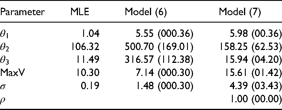
An important talking point throughout this investigation is that field data do not provide reliable measurements $y_t$ for larger time durations $t$ . To check the sensitivity of the estimates in Table 2, we repeat the analyses based on a larger sample size of $n=15$ observations $y_1,\dots ,y_{15}$ . Table 3 provides the estimation results with the larger sample size. We now observe that CV-3 estimates are unreasonable in each of MLE, Models (6) and (7) contexts. For example, the critical velocity ${\theta }_1$ is too low under MLE, ${\theta }_2$ and ${\theta }_3$ are inconsistently large in Model (6), and MaxV is impossibly large for Model (7).

Table 3.

Estimates of CV-3 model parameters (and standard errors) based on MLE, the intial Bayesian model (6) and the enhanced Bayesian model (7) when $n=15$ observations $y_t$ are utilized. The parameter $\mathrm{MaxV}={\theta }_1+{\theta }_2/{\theta }_3$ denotes maximum instantaneous velocity.

Parameter	MLE	Model (6)	Model (7)
${\theta }_1$	1.04	5.55 (000.36)	5.98 (00.36)
${\theta }_2$	106.32	500.70 (169.01)	158.25 (62.53)
${\theta }_3$	11.49	316.57 (112.38)	15.94 (04.20)
MaxV	10.30	7.14 (000.30)	15.61 (01.42)
$\sigma$	0.19	1.48 (000.30)	4.39 (03.43)
$\rho$			1.00 (00.00)

A drawback of the illustration in this section is that long distance runners (upon which the prior is based) most likely have different critical velocity characteristics than the soccer player of interest. In practice, it is important that the prior describes a realistic probabilistic description of the athlete of interest. We have tried to mitigate the shortcomings of our dataset by using a more diffuse prior (i.e. using $k\mathrm{\Sigma }$ instead of $\mathrm{\Sigma }$ with $k=1.5$ ). In practice, how might a user select $k$ ? As a tuning parameter, one might consider various choices of $k>0$ and compare various posterior estimates as reported in Table 2. If the parameter estimates are non-sensical and too precise (i.e. small standard errors), this suggests that the prior is dominating the data and that $k$ needs to be larger. However, if $k$ becomes too large, then the inferences are essentially based only on the data $y_1,\dots ,y_n$ , and with small $n$ , it is difficult to reliably fit a three-parameter model. If one was really confident in the prior, then choosing $k<1$ may be appropriate; this would have the effect of moving posterior estimates closer to prior estimates.

In our Bayesian formulation, the specification of reliable prior information provides a key role, and we have outlined an approach using parameter estimates from other athletes. Of course, prior information may arise from other sources including expert knowledge, and this knowledge may be incorporated into the prior distributions.

Discussion

The main contribution of this paper is the estimation of CV-3 parameters with inexpensive field data. The challenge is that field data are unreliable for larger time durations $t$ . Therefore, only minimal field data are used (based on smaller time durations) where the data are supplemented with prior information.

Moving forward, how might one improve estimation? An obvious strategy involves the improvement of prior knowledge, and this may be accomplished by setting hyperparameters based on athletes who are more similar to the athlete in question. Another avenue is through improved models. We have provided careful investigation of model assumptions including the conditional independence of the data $y_t$ . One may consider alternative models that have been proposed in the critical power literature. Another possibility involves the design of training sessions where athletes are required to move at maximal speeds for longer time durations. This would permit the inclusion of data $y_t$ for larger values of $t$ .

In the context of field data, we have also investigated the use of the ubiquitous maximal moving average Equation (2) as an approximation to maximal sustainable velocity (see Appendix A). We have observed that the formula may not be ideal for larger time durations. There is also the suggestion that modified training schedules may help improve the approximation.