Sage Journals: Discover world-class research

Abstract

More experience results in better performance, usually. In most tasks, the more chances to learn we have, the better we are at it. This does not always appear to be the case in time perception however. In the current article, we use three different methods to investigate the role of the number of standard example durations presented on performance on three timing tasks: rhythm continuation, deviance detection, and final stimulus duration judgement. In Experiments 1a and 1b, rhythms were produced with the same accuracy whether one, two, three, or four examples of the critical duration were presented. In Experiment 2, participants were required to judge which of four stimuli had a different duration from the other three. This judgement did not depend on which of the four stimuli was the deviant one. In Experiments 3a and 3b, participants were just as accurate at judging the duration of a final stimulus in comparison to the prior stimuli regardless of the number of standards presented prior to the final stimulus. In summary, we never found any systematic effect of the number of standards presented on performance on any of the three timing tasks. In the discussion, we briefly relate these findings to three theories of time perception.

Keywords

Time perception rhythm continuation duration deviance detection exposure effects scalar expectancy theory dynamic attending theory

Introduction

We have all had the experience of watching a movie for the second time; we notice a knife on the table, a sideways glance by the antagonist, a Pepsi that doesn’t belong in the medieval period. Seeing things more than once can help attune us to details we missed the first time around. More generally, repetitive exposure improves performance on a range of tasks. In formal experimental settings, it has long been known that repeating items to be learned improves many aspects of their memorisation (for reviews, see Hintzman, 1976 and Hintzman & Block, 1971). More recently, this has shown to be the case even with items not available to conscious perception (Pang & Elntib, 2021), a testament to the strength of the repetition effect on memory. Likewise, repeating motor skills has been found to improve them (Wulf, 2007).

In this article, we are interested in how the short-term repetition of timed intervals affects our ability to notice deviations in duration. In both audition (e.g., Bader et al., 2017, 2021; Cowan et al., 1993; Garrido et al., 2008; Ulanovsky et al., 2003; Winkler et al., 1996) and vision (Atas et al., 2013; Pang & Elntib, 2021), the repetition of stimuli improves the perception of change, as shown by both neural and behavioural methods. This has been formally described using Bayesian observer models (Mathys et al., 2014; Weber et al., 2020) in which the number of repetitions prior to a change alters the surprise induced by said change and alters the perception of a stimulus depending on its recency (Fritsche et al., 2020).

Despite the work in other domains of perception, little work has been done on the effects of repetition on perceived time. In temporal generalisation, L. A. Jones and Wearden (2003; see Wearden, 1992, for a simple version) showed that an initial exposure to 1, 3, or 5 examples of an auditory interval did not significantly affect performance. This indicated that more exposures to an example interval did not improve perception of other intervals across an entire experiment. This has also been shown to be the case in the visual domain (Ogden & Jones, 2008). At the single-trial level, Ogden and Jones (2008) also demonstrated that 1, 3, or 5 repetitions of an interval to be reproduced did not improve the accuracy of reproduced intervals, ranging in time from 110 to 1141 ms. However, it should be noted that a single repetition did lead to systematically shorter reproductions, suggested to be due to the participants missing the start of the visual stimulus as they were not prepared for it (this contention is further supported by Wehrman, 2020a). A third experiment tested this idea by cueing the arrival of the stimuli, and in this case there was no significant difference in the reproductions as a function of the number of standards presented. In Experiment 1 of this article, we attempt to replicate the temporal reproduction findings of Ogden and Jones (2008) using a “ready, set, go” task that will be described below, but is basically similar to that used by Jazayeri and Shadlen (2010). In line with the article by Ogden and Jones (2008), we do not expect an effect of the number of repetitions on the durations produced in our “ready, set, go” paradigm.

Exemplar selection

The explanation given by L. A. Jones and Wearden (2003) and Ogden and Jones (2008) for why there is no performance improvement given multiple exemplars is relatively simple. Generally, across multiple experiences, humans are fairly accurate at timing an interval. However, this requires a number of attempts; on any given trial, perceived time can vary quite widely. If subjects “average” their experiences together, then given more examples of a given duration, their perception should improve. However, given that these prior articles did not find such an effect, it was proposed by L. A. Jones and Wearden (2003), that perhaps rather than averaging across experiences, people simple select one example out of all those shown to them. Furthermore, as implied by other theories such as the multiple trace theory (see Los et al., 2014; Los et al., 2016), it may be that the most recent exposure is that which is most likely to be selected. This in itself has interesting implications which will be discussed towards the end of the article however.

Dynamic attending theory

Despite this, at least one theory proposes that time perception should be improved given more repetitions of a given interval. Dynamic Attending Theory (DAT; see Bauer et al., 2015; M. R. Jones, 1976; L. A. Jones & Boltz, 1989; Mathewson et al., 2010; Schroeder & Lakatos, 2009) theorises that increasing the number of standards presented increases entrainment to a given rhythm.¹ The perceptual accuracy of a given stimulus increases the more repetitions a subject is exposed to, as these repetitions entrain the subject more and more into the rhythm of presentation. In the temporal domain, this theory has received some support. In at least three articles (Fromboluti et al., 2013; McAuley & Fromboluti, 2014; McAuley & Jones, 2003), when given a sequence of durations were shown with the same interval between them, the perception of duration deviance (i.e., whether a given stimulus duration was the same as the duration of stimuli) was more accurate when the target duration was in rhythm, rather than out of rhythm. Similarly, when the target duration was not synchronised with the pattern of durations presented, occurring unexpectedly early, the perception of the duration of the interval was shorter than if the target duration occurred in time with the pattern of durations presented.

Dynamic attending theory predictions

However, in these DAT experiments, it should be noted that the number of repetitions is always relatively high. For example, in McAuley and Fromboluti (2014), the sequential position of the target stimulus was either the fifth, sixth, seventh, or eighth repetition. For DAT to hold, we would expect a similar effect after a shorter number of repetitions. In Experiment 1, presented here (the “ready, set, go” paradigm), this theory should propose that as the number of standards presented increased, there should be an improvement in “rhythm attunement” which would lead to more accurate productions given more standards presented. At the very least, given a single presentation of the standard, in which no rhythm is established, durations produced should be worse than given a chance to entrain to the rhythm.

In Experiment 2, we test this by presenting subjects with a deviant duration on either the first, second, third, or fourth presentation of an interval, and ask participants to identify which duration is deviant. If attuning to a rhythm of interval presentation affects perceived duration, we expect to find that the accuracy with which people identify the deviant duration correctly improves given a later position in the sequence, specifically the fourth position, rather than the first or second.

In Experiment 3, we attempt to replicate the experiment by McAuley and Fromboluti (2014), with some changes. In McAuley and Fromboluti (2014), an oddball stimulus was used, which notably distorts the perceived duration of time (Birngruber et al., 2014; Pariyadath & Eagleman, 2012; Wehrman et al., 2018a). In our experiment, we do not alter any dimension of the stimulus aside from its duration. Furthermore, we present the duration at a known location in the sequence, removing the expectational effect, and instead focusing purely on the temporal “rhythm attunement” from the leading sequence. As per Experiment 2, if entrainment does improve the perception of time, we would expect that a longer sequence of intervals prior to the target should improve the accuracy with which the final interval duration is perceived. Furthermore, in line with McAuley and Fromboluti (2014), the final interval is either “in time” with the rhythm of the prior sequence, or either early or late. If entrainment effects the perception of duration, a higher number of repetitions should result in a larger “offbeat” effect, compared with when no such rhythm is established. Specifically, the distortion of the perceived duration should be larger when an interval is presented unexpectedly early when the number of repetitions is higher.

Experiment 1a: ready (ready) set go duration production

Methods

Participants

Participants provided digital consent and all experiments were approved by the Macquarie University Ethics Committee. Twenty-one participants took part (mean age = 20.9 years, SD = 3.9 years, two left-handed, eight male). Sample sizes for all experiments were chosen to match those of previous experiments performed using similar methods (e.g., Wehrman & Sowman, 2021). All subjects were recruited from the SONA participant pool within Macquarie University, and compensated with course credit.

Presenting software

Data were gathered online using the Gorilla Experiment Builder platform (gorilla.sc). See Anwyl-Irvine et al. (2020) for an introduction to the platform and Anwyl-Irvine et al. (2020) regarding time accuracy. This platform has previously been used multiple times for online time perception experiments (see Wearden & Wehrman, 2021; Wehrman & Sowman, 2021). In brief, this platform allows participants to perform experiments in their own home while gathering response times and choices, as well as system information such as operating system and browser details. In the visual modality, the timing of Gorilla has been shown to be comparable with in-person data collection methods (Bridges et al., 2020). Note that stimulus sizes could vary due to differences in screen size for participants. Furthermore, participants were required to complete the experiment on a computer rather than, say, a mobile device.

Procedure

At the beginning of the experiment participants were given detailed instructions about what would occur in each trial. The basic procedure was simple, and participants were shown between two and five circles in a row. The number of circles (i.e., standard durations) presented varied across blocks, and the order of blocks was randomised. Five blocks of each number of standards were presented. On any given trial, the gap between circles varied between 300, 400, 500, or 600 ms (consistent within a single trial). Each of these durations was presented in a random order within a block, such that three sets of each target duration were presented in each block. While the standard durations varied within a block of trials, the number of standards presented was varied between blocks. Participants were given a clear cue as to the number of standards that would be presented per block prior to the initiation of each block. Figure 1 shows the general task format.

Figure 1.

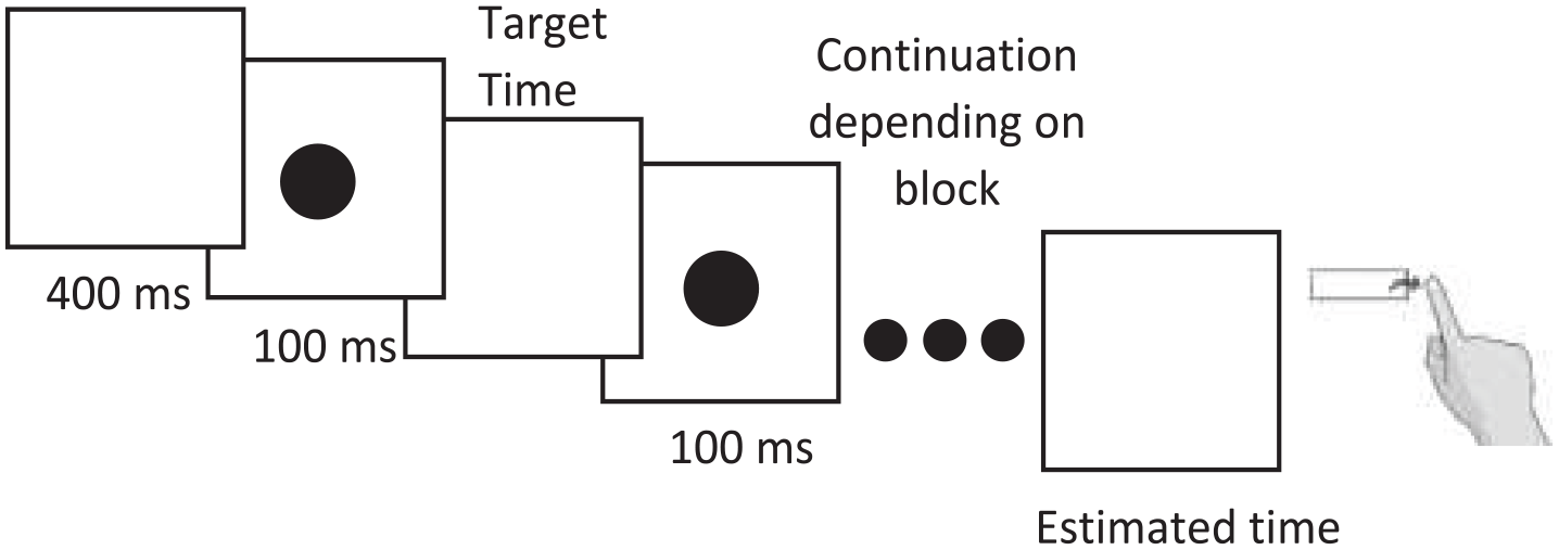
Design of Experiment 1a and 1b. Target time varied by trial, and the number of standards presented (and therefore the number of bracketed times the subject gets) varied by block. Subjects pressed spacebar to terminate the rhythm.

Participants were required to complete the rhythm of the presented standards by pressing spacebar when the next circle completing the final duration would have appeared. A 400-ms blank screen was presented prior to each trial, and each black circle was presented centrally for 100 ms (not included in the gap timing). This task is similar to the task used in Jazayeri and Shadlen (2010), with the exception that the number of standards presented prior to a production varied. As mentioned in the “Introduction,” this experiment seeks to replicate the basic finding by Ogden and Jones (2008), however using a duration production task which continues the rhythm of the intervals presented, rather than breaking the rhythm by asking subjects to both start and stop their reproduction interval.

Analysis

Data were parsed using MATLAB and statistical analysis performed using R and RStudio. Productions of less than a quarter the target duration and longer than four times the target duration were discarded (16.3% of trials). Furthermore, participants whose productions were not systematically increasing to two or more target durations were discarded (e.g., if the durations produced at 200 ms were longer than at 300 and 400 ms: three participants were discarded). An analysis of variance (ANOVA) was performed on the difference between the mean productions and the target duration (to get an error measure) and the coefficients of variation (CVs; standard deviation of durations produced divided by the mean duration produced), with within-subject factors of the target duration and the number of standards presented prior to the production. In addition, we calculated Bayesian statistics (Bayes Factor; BF) using the BayesFactor package in R (Morey et al., 2015). Greenhouse–Giesser (GG) corrections were applied for violations of sphericity where required. Follow-up analysis was corrected with Holm corrections (Holm, 1979). Partial eta squared (η_p²) is reported as a measure of effect size for the ANOVA results, and Cohen’s d (d) is reported for t-tests. Data and code will be made upon request.

Results

The mean duration produced was 555 ms (SD = 245 ms). The main effect of target duration was significant, F(3, 51) = 124.7, p < .001, GG-corrected, η_p² = .88, BF = 1.5 × 10³³. As the target duration got longer, the durations produced also increased (target = production: 300 ms = 456 ms; 400 ms = 505 ms; 500 ms = 591 ms; 600 ms = 669 ms). Furthermore, there was a significant main effect of the number of standards presented, F(3, 51) = 4.57, p = .016, GG-corrected, η_p² = .21, BF = 4.56. As the number of standards increased, so did the durations produced (1 standard = 533 ms, 2 standards = 535 ms, 3 standards = 575 ms, 4 standards = 584 ms). Both these main effects were superseded by interaction effects and were not analysed further.

The interaction between the target duration and number of standards presented, Figure 2a; F(9, 153) = 3.70, p = .006, GG-corrected, η_p² = .18, BF = .106, was further analysed by comparing the durations produced for each target duration given the number of standards presented using ANOVA. At both the 300 ms, F(3, 51) = 1.72, p = .350, Holm-corrected, ηp² = .09, BF = .184, and 400 ms, F(3, 51) = 1.23, p = .350, Holm-corrected, ηp² = .07, BF = .163, the effect of the number of standards was not significant. At the 500 ms target, F(3, 51) = 6.27, p = .004, Holm-corrected, ηp² = .27, BF = 37.1, and 600 ms target, F(3, 51) = 4.57, p = .020, Holm-corrected, η_p² = .21, BF = 17.8, there was an effect of the number of standards. Generally, both these effects show that as the number of standards presented increased, the duration produced increased as well. These results are presented in more detail in the online Supplementary Material.

Figure 2.

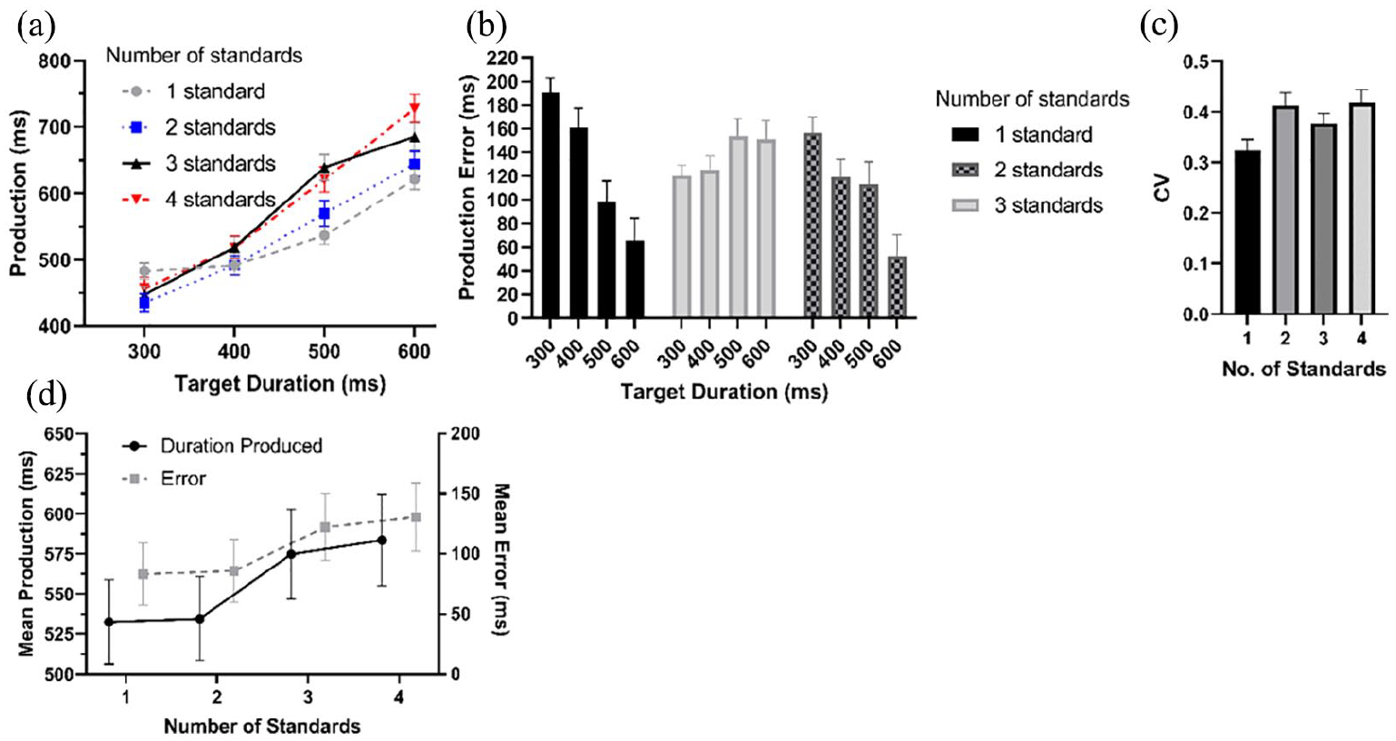
(a) Mean productions at each target duration given the number of standards presented. (b) Mean production difference with target duration, across each target duration and number of standards presented. (c) Mean CV per number of standards presented. (d) Mean duration produced per number of standards (Black) and mean error per number of standards (Grey).

The mean CV (standard deviation of the time produced divided by the mean) was .38. These were significantly affected by the number of standards presented, F(3, 51) = 7.42, p < .001, η_p² = .30; BF = 9.7 × 10³. The CV following one standard (.32) was significantly lower than either two standards, .41; t(17) = 4.11, p = .004, Holm-corrected, d = .50, BF = 24.6, or four standards, .42; t(17) = 3.76, p = .008, Holm-corrected, d = .53, BF = 107.8, but not compared with three standards, .38; t(17) = 2.25, p = .152, Holm-corrected, d = .32, BF = 3.89. No other comparisons were significant (minimum p-value: .152, Holm-corrected, maximum BF = 3.35). This effect is shown in Figure 2c. The main effect of the duration was not significant, F(3, 51) = .779, p = .512, ηp² = .04, BF = .079, and neither was the interaction effect, F(9, 153) = 1.80, p = .646, η_p² = .04, BF = .008.

Experiment 1b

This experiment is a replication of Experiment 1a with the exception of the block order. In this experiment, due to a technical error, participants either performed the three-standard block twice, then the two-standard block, and then the one-standard block, or vice versa. This order of blocks was then repeated five times. Twenty-three subjects took part in this experiment (mean age = 19.6 years, SD = 2.1 years, three left-handed, 11 male).

Analysis was as above. In this experiment, 17.7% of trials were discarded as outside the quarter to four-times range. Two participants were also removed for having more than one non-monotonically increasing duration production.

Results

The mean duration produced was 579 ms (SD = 118 ms). The main effect of target duration was significant, F(3, 66) = 94.9, p < .001, η_p² = .81, BF = 2.2 × 10³⁵. As the target duration got longer, the durations produced also increased (target = production: 300 ms = 448 ms; 400 ms = 533 ms; 500 ms = 630 ms; 600 ms = 705 ms). There was no significant main effect of the number of standards presented in this experiment, F(2, 44) = 1.52, p = .229, η_p² = .06, BF = .109.

The interaction between the target duration and number of standards presented, Figure 2a and d; F(6, 132) = 7.57, p < .001, GG-corrected, η_p² = .26, BF = 1.63, was further analysed by comparing the durations produced for each target duration given the number of standards presented using ANOVA. At the 400 ms, F(2, 44) = 2.50, p = .188, Holm-corrected, ηp² = .10, BF = .747, and 500 ms, F(2, 44) = 2.23, p = .188, Holm-corrected, ηp² = .09, BF = .632, target durations, the effect of the number of standards presented did not significantly affect productions. At the 300 ms target, F(2, 44) = 4.54, p = .049, Holm-corrected, ηp² = .17, BF = 3.20, and 600 ms target, F(2, 44) = 10.43, p < .001, Holm-corrected, η_p² = .32, BF = 126.9, there was an effect of the number of standards. While there was a general trend for a longer duration to result in longer productions at both these numbers of standards, the results were less orderly than in Experiment 1a. Detailed results are presented in the online Supplementary Material.

The mean CV was .43. This was significantly affected by the target duration, F(3, 66) = 3.13, p = .031, η_p² = .12, BF = .742. However after Holm correction, no CV difference between the target durations was found (minimum p-value: .051, Holm-corrected, maximum BF = 2.09). The main effect of the number of standards was also significant, F(2, 44) = 6.45, p = .003, ηp² = .23, BF = 16.4. CVs were significantly smaller given one standard (.40) compared with the three standards, .45; t(22) = 3.82, p = .002, Holm-corrected, d = .34, BF = 37.5. Neither difference was significantly different compared with the two-standard condition (.43; minimum p-value: .170, Holm-corrected, maximum BF = .876). The interaction effect was not significant, F(6, 132) = .722, p = .633, η_p² = .03, BF = .038. Both main effects are show in Figure 3b and c, respectively.²

Figure 3.

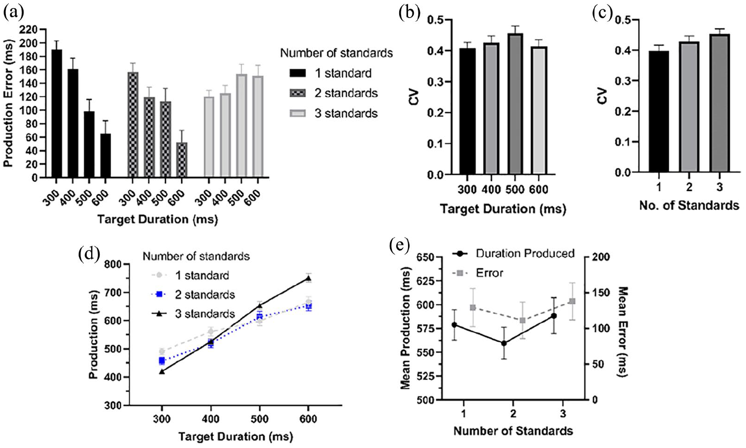
(a) Mean production difference with target duration, across each target duration and number of standards presented. (b) Mean CV by target duration. (c) Mean CV by the number of standards presented. (d) Mean productions at each target duration given the number of standards presented. (e) Mean duration produced per number of standards (Black) and mean error per number of standards (Grey).

Discussion

In these experiments, we varied the number of exemplar durations presented prior to the production by the subject. The results here largely support the findings by L. A. Jones and Wearden (2003) and Ogden and Jones (2008): timing performance does not appear to improve as the number of standards presented increases. In fact, the opposite appears to be true in Experiment 1a; given one or two standard durations (i.e., two or three circles), the performance was closer to the objective target duration compared with when three or four standard durations (i.e., four or five circles) were presented. In Experiment 1b, there was no significant relationship between the number of standards presented and the mean duration produced. However, in both experiments, effects obtained are complicated by the target duration produced. In Experiment 1a shorter target durations of 300 or 400 ms appeared fairly consistently produced, despite the number of standards presented, while at 500 and 600 ms, an increasing number of standards appeared to gradually increase the error produced. In Experiment 1b, however, 400 and 500 ms targets were relatively consistently produced. The 300 ms target was produced as shorter (i.e., more accurately) given more standards, while at 600 ms, the opposite was true.³

It is worth noting that perhaps our results are due to participants miscounting the number of standards presented, especially with the presentation of more standards. However, we discount this possibility in two regards. First, if subjects were miscounting the number of standards, then we would expect a larger number of extreme productions as the number of standards increased. In the online supplementary material, we present histograms of production errors and summary statistics of the number of extreme productions. It does not appear that the number of extreme productions increased uniformly with the number of standards. Second, in Experiment 1b, participant errors were approximately the same whether given a single example of a duration, or three examples of that duration. Indeed, while one could argue that perhaps this effect is greatest at the longest durations (e.g., 600 ms, where the time to notice a missing circle should be longest), Experiments 1a and 1b show contrasting results in this regard as well; with a relatively smaller error in Experiment 1b compared with Experiment 1a. Together, these seem to discount the possibility of participants simply “missing” the production.

Importantly, while Ogden and Jones (2008) required their participants to reproduce the entire interval, in our experiment, people were expected to “complete the rhythm,” thereby relying on rhythm entrainment rather than pure duration replication. In this way, DAT also has a clear hypothesis for this experiment; given more entrainment, the perception of duration, that is, reproduction, should be more accurate. This was not the case, more examples, and thus a better chance for people to attune to the rhythm of the task, did not result in more accurate reproductions.

In Experiment 2, we presented participants with four circles, and asked them to detect which circle was presented for a different duration from the other three, the standards. If rhythm entrainment, or simply more exposure, results in a better ability to detect duration deviance, then we would expect that as more standards are presented, participants will become more accurate at detecting deviant durations the later in the series the target is presented.

Experiment 2: deviance detection

Methods

Participants

Twenty-one participants took part in this experiment (mean age = 19.8 years, SD = 2.6 years, one left-handed, seven male).

Procedure

Each trial, the participants were shown four black circles located centrally, separated by a 400-ms blank screen. Three of the circles presented had a 400-ms duration, and one of them was presented for 150, 200, 280, 350, 450, 520, 600, or 650 ms. At the end of the trial, the participants were shown “1 2 3 4 ?” to which they responded with the numbers on their keyboard as to which circle was presented for the odd amount of time. Each block consisted of 32 trials, one of each duration at each circle, presented in random order. 10 blocks of trials were given. Figure 4 shows design of Experiment 2.

Figure 4.

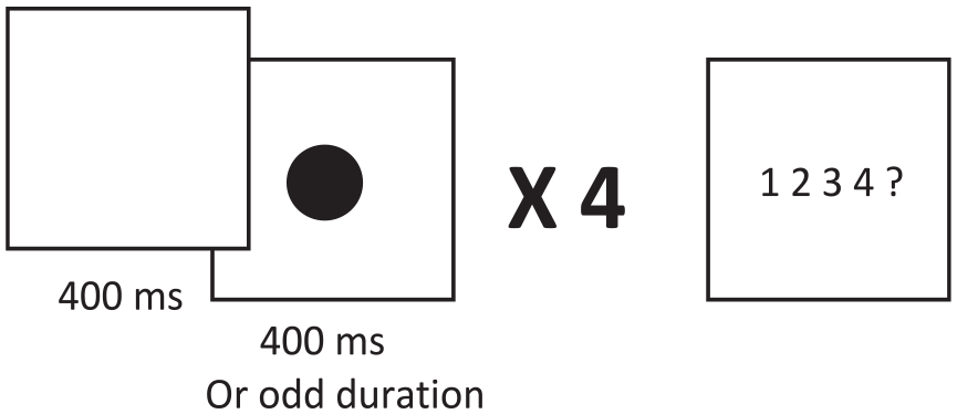
Design of Experiment 2. Subjects were shown four circles, three of which were 400 ms, and one of which had an odd duration of 150, 200, 280, 350, 450, 520, 600, or 650 ms. When the phrase “1 2 3 4 ?” appeared, subjects had to press the number corresponding to the circle which had an odd duration.

Analysis

As in Experiment 1, data were parsed using MATLAB and statistical analysis performed using R and RStudio. Because the task was completed at home, trials in which decisions took longer than 5 s were discarded as possibly “distracted” trials (2.6% of trials).⁴ Furthermore, any participants who did not obtain at least 50% correct on the 150 ms trials, or 25% correct on the 650 ms trials (because the trials were spaced arithmetically, these were subjectively harder than the 150 ms trials) were discarded as unlikely to have been paying attention (four participants). The mean percentage of correct responses per participant per target and duration were then calculated.

The point of maximal uncertainty (PMU) was also calculated (see Birngruber et al., 2014, 2017; Dyjas & Ulrich, 2014; Wehrman et al., 2018a, 2020, for discussion and application of this method). This is essentially finding the duration at which reaction times (RTs) were longest. The maximum (i.e., longest) RT is found using waveform moment analysis (Cacioppo & Dorfman, 1987), and allows identification of the duration at which subjects are least confident in their responses.⁵ This normally corresponds to the point at which subjects make the most mistakes in their responses, and gives further validation of that result (see Balcı & Simen, 2016; Simen et al., 2011).

Results

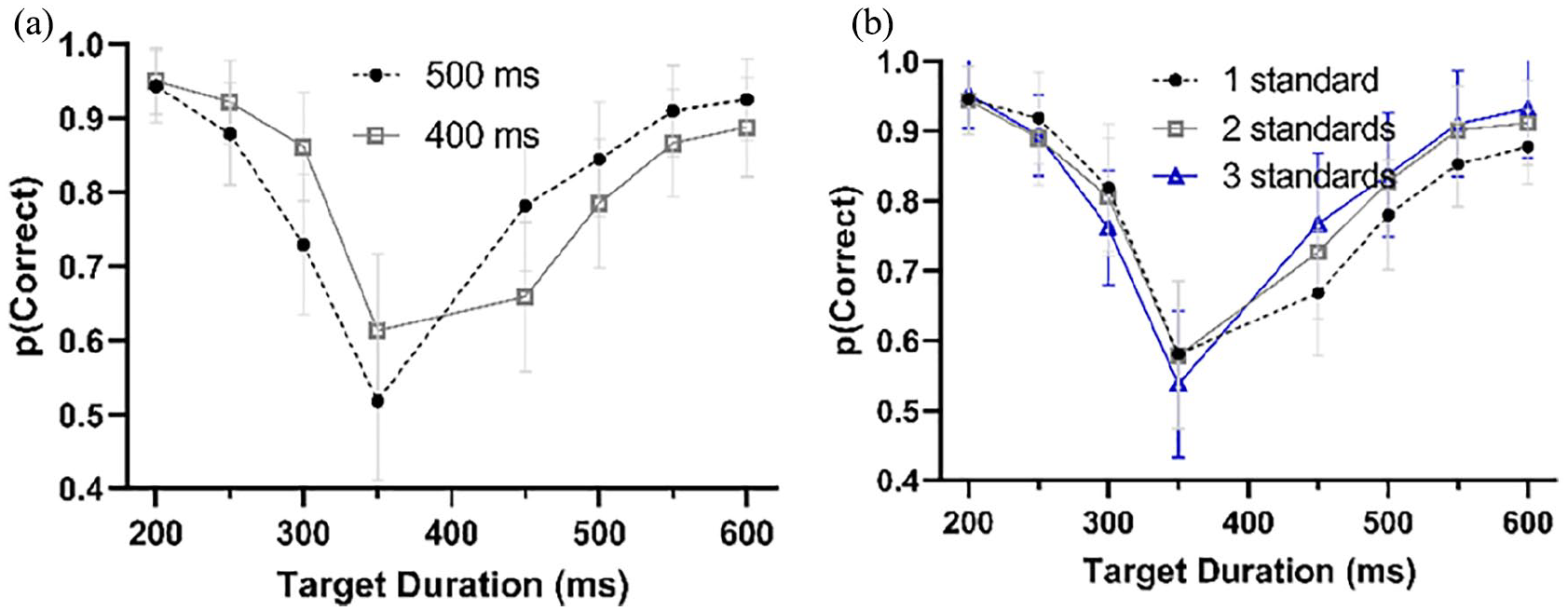
On average, subjects were correct on 49.8% of trials overall (SD = 8.8%). Accuracy was significantly affected by the duration of the target, F(7, 140) = 78.1, p < .001, GG-corrected, η_p² = .80, BF = 5.7 × 10¹⁰⁰. This effect was as expected, as the target durations further from the 400 ms standard, would be expected to be easier to identify.⁶ There was also a main effect of which circle had the deviant duration, F(3, 60) = 3.64, p = .036, GG-corrected, η_p² = .15, BF = .220. Participants were correct 50.9% of the time if the target was the first circle, 47.5% if the second circle, 53.8% if the third circle, and 46.7% if the fourth circle. This result is shown in Figure 5b. Both these main effects were superseded by an interaction effect and were not analysed further.

Figure 5.

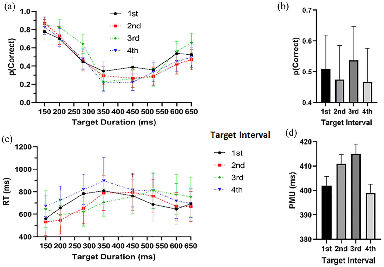
(a) Proportion of correct responses per target circle and target duration. (b) Proportion of correct responses per target circle. (c) Mean RT per target circle and target duration. (d) Mean PMU per target circle.

The interaction effect between the target duration, and which circle was the deviant duration was also significant, F(21, 420) = 3.39, p < .001, GG-corrected, η_p² = .14, BF = .018. To further analyse this interaction, we performed an ANOVA at each time point, across the number of standards presented. Following correction for multiple comparisons, only the 280 ms, F(3, 60) = 6.09, p = .009, η_p² = .23, BF = 38.4, and 650 ms, F(3, 60) = 5.18, p = .021, η_p² = .23, BF = 12.9, ANOVAs remained significant (i.e., only at these two time points, was there an effect of which circle was of a deviant duration). The remaining time points did not show significant effects of the number of standards.⁷ Due to the inconsistency of effects, no further comparisons were made. These results are shown in Figure 5a.

The mean PMU was 406 ms, corresponding relatively closely to the actual mean target duration of 400 ms of the standard stimuli. The PMU was significantly affected by which number target was of a deviant duration, F(3, 60) = 4.49, p = .007, η_p² = .18, BF = .166. Following Holm-correction, only the comparison between the first and third target, t(20) = 2.89, p = .049, Holm-corrected, d = .77, BF = 1.25, and third and fourth target, t(20) = 2.93, p = .049, Holm-corrected, d = .95, BF = 4.08, were significant. This is shown in Figure 5c and d. Again, however, the key point here is that which circle had the deviant duration did not systematically affect responses.

Discussion

In this experiment, there was no systematic effect of which circle had the deviant duration on the probability of a subject correctly identifying the deviance. That is, there was no simple repetition effect observed. The results of this experiment did however follow several common patterns in time perception, for example the skewed temporal generalisation curve in which deviance detection is superior when the deviant is shorter rather than longer than the standard (e.g., Bannier et al., 2018; Droit-Volet & Izaute, 2005; Wearden & Bray, 2001) and increasing uncertainty, as measured by the PMU, as the target time gets closer to the objective midpoint (e.g., Wehrman et al., 2018a, 2020). Most temporal generalisation or deviance-type tasks use only two stimuli, the first of which is a standard and the second of either the same or deviant duration. While expected, it is interesting to note that the common pattern of findings was also present in the current four-stimulus type task.

If viewing this experiment under DAT, one could argue that perhaps the “beat is caught” across trials, and that after a few trials, the participant is sufficiently attuned to the rhythm so that more standards do not affect performance. However, this account seems unlikely due to the large breaks in rhythm presented by the intervals which are not in keeping with the rhythm (and the intertrial interval). Generally, a stimulus resets oscillators (i.e., a phase reset) such that oscillators are synchronised by external stimuli (see, for example, the steady state visual evoked potential, Norcia et al., 2015 present a recent review). This is the basis for DAT; repeated stimulation reinforces entrainment. However, in the current experiment, this entrainment is broken every trial, and thus must be reset. Similarly in DAT experiments (e.g., McAuley & Fromboluti, 2014) seem to make a similar assumption that an “odd” duration will require a reset of rhythmic entrainment (as otherwise entrainment would reach an asymptote, and no effects of position would be seen for “on time” presentation of a stimulus, see Figure 5 of McAuley & Fromboluti, 2014).

In the final two experiments, we examined the possible effect of the number of standard intervals between durations on the perception of the duration of the final circle. In these two experiments, people were presented with two, three or four circles with a standard duration between each of 400 ms. Each of these circles (i.e., standards) was presented for a standard of 400 ms duration as well. The final circle however was presented for a variable duration, and with either an earlier-than-expected (Experiment 3a) or later-than-expected (Experiment 3b) gap between the final circle and the immediately preceding circle. This final set of experiments was designed as a replication of the study by McAuley and Fromboluti (2014). However, while McAuley and Fromboluti (2014) “guaranteed” entrainment by the presentation of several intervals prior to the target interval, we offered the possibility of no entrainment. The hypothesis for these experiments is clear, if entrainment explains any repetition effect in time perception, then given a single example interval the subjects should be less accurate in their perception than given a chance to entrain to the duration. In addition, the disruption caused by an out-of-sync final interval should be larger once a person has entrained to the durations presented (i.e., at four presentations) rather than when no entrainment is provided (i.e., given a single example).

Experiment 3a: final circle perception with negative offset

Methods

Participants

Twenty-two participants took part in this experiment (mean age = 20.5 years, SD = 4.3 years, 10 male, two left-handed).

Procedure

In this experiment participants were required to judge whether the duration of the final circle was shorter or longer than the preceding circle. On each trial, subjects were shown either two, three, or four black circles presented centrally (varied by block, and presented in random order such that each block was presented five times in total). All but the final circle was presented for 400 ms, and all but the final circle was separated by 400 ms from the previous one (similar to McAuley & Jones, 2003). The final circle was preceded by either the standard interval between circles (400 ms) or a slightly shorter interval (300 ms; that is, off-rhythm). The final circle lasted either 200, 250, 300, 350, 450, 500, 550, or 600 ms, followed by a 150 ms blank screen and a screen saying “(S)horter or (L)onger?” prompting the participant to respond with either the S or L key if they thought the final circle was shorter or longer than the preceding circle, respectively. In each block, each combination of gap duration and circle duration was presented twice. Figure 6 shows a schematic of the procedure. Notably, this experiment provides a conceptual replication of McAuley and Fromboluti (2014), however the target duration is always the final duration in the train (removing the effects of expectation, instead focusing only on entrainment) and is not an oddball, i.e., does not vary in any other regard other than duration.

Figure 6.

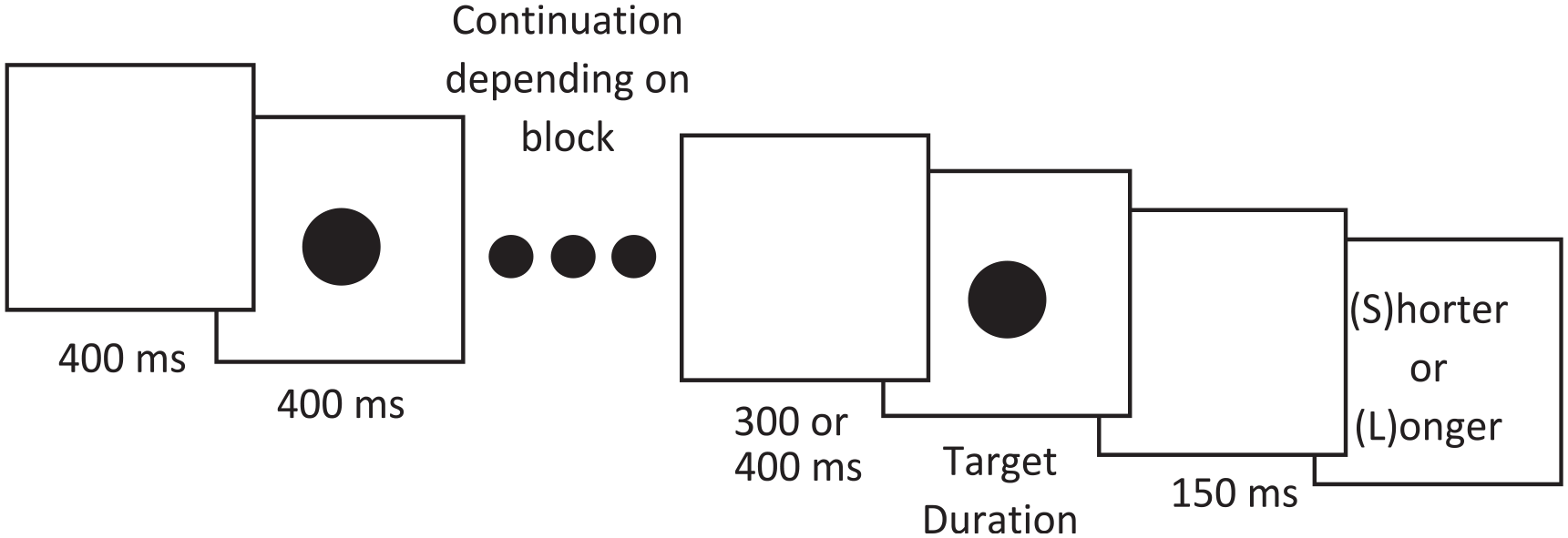
Design of Experiment 3a and 3b. Target time varied by trial, and the number of standards presented (and therefore the number of bracketed times the subject gets) varied by block. Subjects pressed spacebar to terminate the rhythm.

Analysis

Reaction times shorter than 50 ms (from the offset of the target) or longer than 5000 ms were discarded as preemptive and a lapse of attention, respectively (6.1% of trials). In MATLAB, we then used psignifit to fit a cumulative Gaussian distribution to participant choices for each combination of the number of standards presented, and the gap between the final and previous circles. From this, we extracted the point of subjective equality (PSE), the duration at which people were equally likely to choose short and long.⁸ We also calculated the Weber ratio (WR) as half the difference between a 75% and 25% response difference, divided by the PSE. The effects in terms of the percentage of “Long” decisions for both Experiments 3a and 3b are presented in the supplementary appendix.⁹

Results

Participants chose “Long” 48% of the time on average (SD = 7.1%) and were correct 75% of the time on average (SD = 13.1%). The percentage correct responses in terms of the final offset and the number of standards are shown in Figure 7a and b, respectively.

Figure 7.

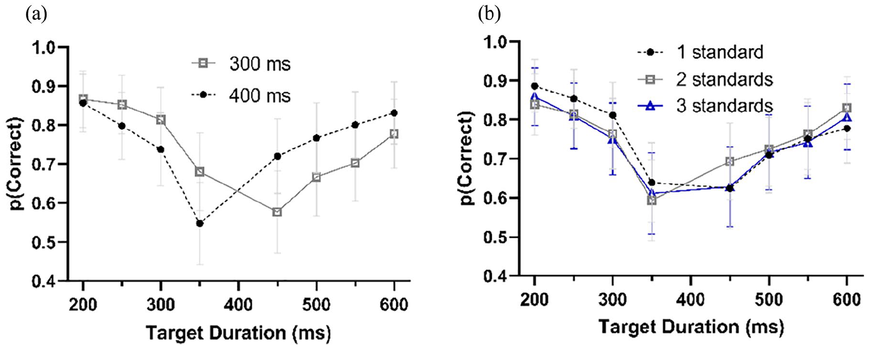
(a) Correct responses given a 300- or 400-ms gap between the second to last and last circle in the series. (b) Correct responses given the number of standards presented on a given trial.

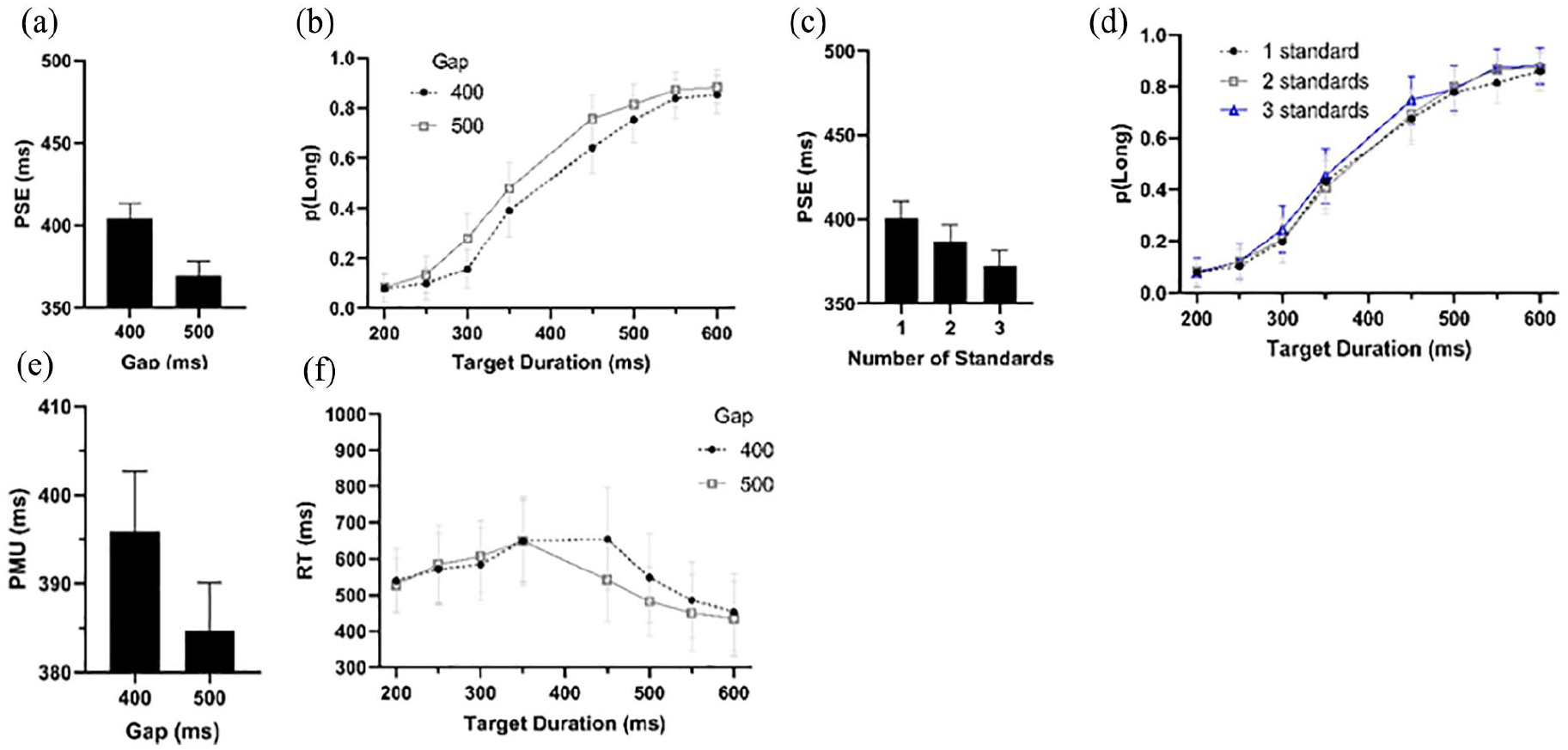
The mean PSE, the point at which participants subjectively judged the midpoint of the durations presented was 401 ms. This was not significantly different than the objective midpoint of 400 ms, t(21) = .008, p = .993, d < .01, BF = .223. The PSE was not significantly affected by either the number of standards presented, F(2, 42) = .889, p = .386, GG-corrected, ηp² = .04, BF = .091, or the interaction between the number of standards and the gap between the final and second to last circle, F(2, 42) = .088, p = .854, GG-corrected ηp² < .01, BF = .176. The main effect of the gap was significant, however, F(1, 21) = 8.90, p = .007, η_p² = .30, BF = 9.40, showing that if a shorter-than-expected gap was presented, the PSE was significantly later (427 ms) compared with if the gap was the expected 400 ms (374 ms). This is shown Figure 8a. Figure 8d shows effects on PSE of the number of standards presented, for comparison with Experiment 3b.

Figure 8.

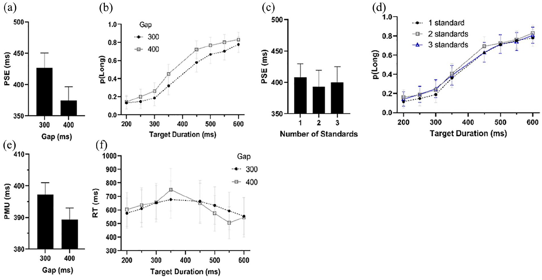
(a) PSE given a 300- or 400-ms gap between the second to last and last circle in the series. (b) Percentage Long choices given each target time and the gap. (c) PSE given number of standards prior to the deviant duration. (d) Probability of correctly choosing whether a given target was shorter or longer than the standard. (e) PMU given a 300- or 400-ms gap between the second to last and last circle in the series. (f) Mean RTs over each target duration and gap.

The mean WR was .444. However this was not affected by the number of standards, F(2, 42) = .339, p = .714, ηp² = .02, BF = .105, the gap, F(1, 21) = 1.94, p = .179, ηp² = .08, BF = .325, or the interaction between the two, F(2, 42) = .419, p = .660, η_p² = .02, BF = .168.

The mean PMU was 393 ms. This was not significantly affected by either how many standards were presented, F(2, 42) = .229, p = .796, ηp² = .02, BF = .105, or the interaction with the gap between the final and second to last circle, F(2, 42) = .560, p = .576, ηp² = .03, BF = .168. The main effect of this gap was significant, however, F(1, 21) = 6.88, p = .016, η_p² = .25, BF = .325, such that the PMU was later following a 300-ms gap (397 ms) rather than a 400-ms gap (389 ms). This is shown in Figure 8e.

Experiment 3b: final circle perception with positive offset

Methods

Twenty-two participants took part in this experiment (mean age = 18.1 years, SD = 1.0 years, two male, one left handed).

The procedure was as per Experiment 3a except the gap between the final and proceeding circle was either 400 or 500 ms. The analysis was performed as above, with 2.3% of trials being discarded.

Results

Participants chose “Long” 51% of the time (SD = 5.2%), and correctly chose whether a duration was short or long 82% of the time (SD = 6.3%). The percentage correct responses in terms of the final offset and the number of standards are shown in Figure 9a and b, respectively.

The mean PSE was 387 ms. This was slightly lower than the objective central duration of 400 ms, t(21) = 2.10, p = .048, d = .45, BF = 1.38. The mean PSE was significantly affected by the number of standards presented, F(2, 42) = 5.71, p = .006, ηp² = .21, BF = 11.1, with fewer standards resulting in a later PSE (one standard = 401 ms, two standards = 387 ms, three standards = 373 ms). However, only the difference between the one and three standards condition was significant, t(21) = 2.95, p = .008, Holm-corrected, d = .73, BF = 6.19, the other two comparisons did not reach significance (minimum p = .132, Holm-corrected, maximum BF = 1.08). This is shown in Figure 10d.

Figure 9.

(a) Correct responses given a 400- or 500-ms gap between the second to last and last circle in the series. (b) Correct responses given the number of standards presented on a given trial.

Figure 10.

(a) PSE given a 400- or 500-ms gap between the second to last and last circle in the series. (b) Percentage Long choices given each target time and the gap. (c) PSE given number of standards (d) Probability of correctly choosing whether a given target was shorter or longer than the standard. (e) PMU given a 400- or 500-ms gap between the second to last and last circle in the series. (f) Mean RTs over each target duration and gap.

The main effect of the gap was also significant, F(1, 21) = 30.15, p < .001, η_p² = .59, BF = 1.1 × 10⁵, showing that if the standard gap (400 ms) was presented, the PSE was significantly later (404 ms) compared with if the gap was longer (370 ms). This is shown in Figure 10a. The interaction between the number of standards and the gap between the final and second to last circle was not significant, F(2, 42) = .165, p = .848, η_p² < .01, BF = .132.

The mean WR was .438. However this was not affected by the number of standards, F(2, 42) = .087, p = .917, ηp² < .01, BF = .078; the gap, F(1, 21) = .224, p = .641, ηp² = .01, BF = .200; or the interaction between the two, F(2, 42) = .966, p = .389, ηp² = .04, BF = .294. The mean PMU was 390 ms. This was not significantly affected by how many standards were presented, F(2, 42) = .232, p = .794, ηp² = .01, BF = .342, or the interaction with the gap, F(2, 42) = .054, p = .951, ηp² < .01 BF = .161. The main effect of the gap was significant, F(1, 21) = 7.06, p = .015, η_p² = .25, BF = 8.10, such that the PMU was later following a 400-ms gap (396 ms) rather than a 500-ms gap (385 ms). This is shown in Figure 10e and f.

Discussion

As in Experiments 1a and b and Experiment 2, there was no systematic effect of the number of standards presented on the perception of duration of the final stimulus, that is, no simple repetition effect. The number of standards presented did not affect the probability of detection of the deviant stimulus, even when the position of the deviant stimulus is known (i.e., always the last stimulus). Furthermore, the effect of the gap between the final stimulus and the previous stimulus did not depend on the number of stimuli presented. As in Experiment 2, it is worth noting that standard findings are replicated, including longer response latencies as the decision becomes more difficult, and the probability of being correct skewing slightly earlier than the objective midpoint (e.g., Bannier et al., 2018; Droit-Volet & Izaute, 2005; Wearden & Bray, 2001).

When the timing of presentation of the last stimulus was altered, there was a systematic shifting of the PSE; the longer the gap, the lower the PSE (though the actual values depended on the experimental context, with a 400-ms gap resulting in a relatively lower or higher PSE in Experiments 3a and 3b, respectively). This lower PSE indicates that, to reach the subjective point at which the durations are equally likely to be short or long, a shorter amount of time is required than objectively the case, and thus that time is perceived to pass faster in the “longer gap” condition. Furthermore, while the actual peak of incorrect responses was only somewhat shifted in time, the probability of correct responses was significantly lower as the offset of the last stimulus was shifted later. This is in line with other findings from the oddball duration illusion in which expectation leads to a longer perceived duration (e.g., Birngruber et al., 2017; Wehrman et al., 2018a). When the final stimulus is presented earlier than expected, there is no way to predict when it will be shown. In this case, once the 300-ms time has passed however, the final stimulus is guaranteed to occur 100 ms later, that is, at 400 ms. Similarly, in Experiment 3a, once the 400-ms standard gap has passed, the final circle is guaranteed to occur at 500 ms, and therefore is entirely predictable. This hazard effect (see Janssen & Shadlen, 2005; Nobre et al., 2007) has previously been shown to expand the perceived duration of oddball stimuli (Wehrman, 2020b; Wehrman et al., 2018a), a finding supported here (though here with repeated stimuli, resulting in smaller effects).

Finally, it is worth noting that the later PMU following an earlier gap was expected, given that a rhythm was set up and thus response times were likely slower. This does seem to show that participants were learning to expect when the final stimulus would occur, in line with the expectation effects described above. Despite these expectations being formed however, there still did not appear to be a systematic effect of the number of stimuli presented.

General discussion

The three experiments presented above use different methods, rhythm production in Experiments 1a and 1b, deviance detection in Experiment 2, and a Longer/Shorter judgement in Experiments 3a and 3b, yet all had a common result: Increasing the number of standards presented did not improve performance systematically, there was no “simple repetition” or “entrainment” benefit. As in L. A. Jones and Wearden (2003) and Ogden and Jones (2008), exposure does not improve performance.

Dynamic attending theory

The findings of all three experiments run counter to the intuition proposed under DAT. In Experiment 1, if entrainment resulted in better temporal resolution, then a rhythm continuation should be more accurate after four repetitions of the same example duration, than after one repetition. This was not the case, and at longer durations (akin to the durations used in McAuley & Jones, 2003), there was some indication that a single instance was produced more accurately than given multiple examples. Under DAT, in Experiment 2, it could be argued that duration deviance in either the first or final circle should have been more clearly perceived (due to an entrainment effect prior to, or after, the deviant). Again, there was no such trend in the data. Finally, in Experiment 3, in the closest replication to the DAT experiments which show improved temporal perception for in-rhythm presentations, we found that while the number of standards did not alter the perception of time, the gap prior to the final target duration did. Rather than an effect of entrainment, one simple explanation for this could be that people add or subtract some percentage of the amount of time they were expecting to wait prior to the final stimulus being presented to their perception. This is generally in line with findings such as Wehrman (2020b) where it was shown that timing does not necessarily start with the objective start of a stimulus.

However, while we failed to find support for DAT, it is possible that at longer durations of stimuli (i.e., supra-second) or the gap between stimuli, that entrainment may be stronger. Indeed, there is now substantial neuroimaging and behavioural evidence that timing seems to be performed differently above around 1 s (Hayashi et al., 2014; Nani et al., 2019). This is deserving of further study; however, it is notable that, at least in terms of DAT, McAuley and Jones (2003) had used a similar duration range to that used here.

Random selection

Instead, the results of the current experiments seem more in line with participants selecting one of the standards presented and using this as the basis for their performance rather than an averaging of exemplars, as proposed in L. A. Jones and Wearden (2003) and Ogden and Jones (2008). The proposal that perhaps people average their experiences to come to a target performance is an intuitive one; if we see a thousand different blues and a thousand different greens, we can readily categorise them and arrive at a perfect exemplar which is broadly in the middle of these groups (see Woiczyk & Le Mens, 2021, for a recent model of this process). Unfortunately, time and again it appears that, in time perception, this is not the case. Instead, given a thousand different time “blues,” we seem to select one at random, and perform according to the perceived duration of that event.

In particular, Experiment 1 is supportive of people using a sample rather than an average to perform the task. If participants were averaging their duration estimates based on their exposure to the target durations (which changed from trial to trial, disallowing between-trial rhythmic performance), then more standards should result in better performance. This was not the case.

Similarly in Experiment 2, an averaging process should result in better performance in distinguishing duration deviance to the final stimulus, as the prior string of durations are averaged together. This, again, did not appear to be the case. In fact, the identification of deviance was marginally worse when the final stimulus was the target in Experiment 2. A similar argument could be applied to Experiment 3. In this case, it seems likely that the final stimulus gap effect was of different origin than the duration estimation process; while the number of standards presented did not affect perceived duration, the gap did due to perhaps expectation-based effects (see, for example, Wehrman et al., 2018a).

Biased performance

Of course, if there were really one thousand examples of a given duration, it seems unlikely that any of these examples would be selected with equal probability. This raises the possibility of either an average or random selection which is recency-biased. It may be that participants are more likely to randomly select an example that they were more recently exposed to (and the further back the example, the less likely that example is to be selected). Alternatively, the duration estimate may not be a pure average of all prior experiences, but a weighted average such that more recent stimuli have a larger influence on perception. This claim has some basis in time perception research, proposed by Los et al. (2014, 2016) in their multiple trace theory.

A model in which the most recent stimulus is more strongly weighted in contributing to reproduction (Experiment 1) and comparison (Experiments 2/3) would make similar predictions to the random model provided by L. A. Jones and Wearden (2003), with the additional benefit of fitting into the broader literature of sequential presentations, for example, in vision science (Broadbent & Broadbent, 1981; Kalm & Norris, 2018).

Drift diffusion extension

One possible extension to the recency-based interval timing described above is the addition of a drift diffusion process, for example, as proposed by Balcı and Simen (2014, 2016). In this model, timing is not just a single-shot process, but instead made up of two separate random walks. The first is the accumulation of time while the second is a decision process in which a response is approached depending on the final position of the amount of time accumulated in the first process. To combine the drift diffusion model with either random or biased selection of time, the accumulation of time, the initial drift diffusion, could be biased by recent experiences (i.e., drifts faster or slower), or the process could be offset initially (i.e., the starting point is shifted higher or lower). Both these could result in a longer or shorter duration estimate on average. Both the offset and accumulation speed are parameters to the model, and which is affected is an empirical question. The decision process (i.e., the second drift diffusion process) could also then be biased depending on recent experience and responses; see the next section.

The advantage of such a model is that it could take response accuracy and response times, into a single overarching parameterisation which could then explain behaviour over time. Furthermore, applying a drift diffusion model would allow the comparison between time perception and the perception of other aspects of experience, such as how magnitude is processed (e.g., size or length, see Droit-Volet et al., 2008; Wehrman et al., 2020), where drift diffusion modelling has also been applied (see Tavares et al., 2017, for example).

General repetition effects

While we did not find an effect of the number of repetitions on the perceived duration of stimuli in the current experiments, there is evidence that experience does alter perceived duration. For example, anchoring has been documented in the time perception literature (Wehrman et al., 2018b, 2020; Wiener et al., 2014), in which the duration of a previous stimulus affects our perception of the current stimulus. Even some of the earliest time perception investigations have shown a regression to the mean across multiple trials (e.g., Vierordt’s studies of time perception from 1868; see Lejeune & Wearden, 2009). Both these effects clearly show that previous experience and responses have a significant effect on our performance. Similar decisional carryover effects have also been seen in other domains, such as the estimation of shown in the judgement of weight, size, number, and loudness (Bevan & Turner, 1964; Holland & Lockhead, 1968; Larimer, 1965; Parducci & Marshall, 1962; Sherif et al., 1958).

One possible explanation for these effects on time perception in the absence of simple repetition effects is how the durations are used in the tasks. In the experiments performed in this article, as well as L. A. Jones and Wearden (2003) and Ogden and Jones (2008), the simple repetitions are presumably stored as standard durations, that is, the repeated stimuli will be used as a standard for other comparison durations. In the types of tasks in which experience does affect perception, the durations are actively used for judgement (a comparison interval). Perhaps when a comparison is performed between the standard intervals and comparison interval, as per the L. A. Jones and Wearden (2003) model, a random selection of standards is made. However, the perception of the comparison intervals may be adjusted based on prior experience over multiple trials, leading to sequential effects on the perceived duration of the comparison intervals. On a single trial, anchoring occurs (e.g., Wehrman et al., 2020), and over multiple trials, there is a progressive regression to the mean (e.g., Jazayeri & Shadlen, 2010).

Conclusion

Timing is different to other perceptual domains; we have no eye to see time, or ear to hear time. Instead it is a purely cognitive experience. In other domains, such as a vision, being given multiple chances to observe a stimulus may improve performance. In this article, we have demonstrated that merely repeating a given example duration does not improve the perception of time. We propose this to disfavour models such as DAT which rely on entraining to a particular rhythm. Furthermore, a simple averaging of the standard durations does not align with the current findings. Instead, we propose it is most likely that people either take a random sample of the (most recent) durations they are exposed to, and use these for comparison, or compare to an average that is weighted by recency of exposure. To differentiate these possibilities, one future avenue for investigation is the use of the drift diffusion model with a weighted temporal accumulation and perhaps a biased response accumulation. While the perception of time is not improved by multiple examples, which may differentiate time from other perceptions, using a common model to understand timing and other perceptual experiences, how exactly time is different to, for example, vision, may be better understood.

Supplemental Material

sj-docx-1-qjp-10.1177_17470218231157674 – Supplemental material for Can’t catch the beat: Failure to find simple repetition effects in three types of temporal judgements

Supplemental material, sj-docx-1-qjp-10.1177_17470218231157674 for Can’t catch the beat: Failure to find simple repetition effects in three types of temporal judgements by Jordan Wehrman and John H Wearden in Quarterly Journal of Experimental Psychology

Footnotes

Declaration of conflicting interests

The author(s) declared no potential conflicts of interest with respect to the research, authorship, and/or publication of this article.

Funding

The author(s) received no financial support for the research, authorship, and/or publication of this article.

ORCID iD

Jordan Wehrman

Supplementary material

The supplementary material is available at:

Notes

References

Anwyl-Irvine

A. L.

Dalmaijer

E. S.

Hodges

Evershed

J. K.

(2020). Realistic precision and accuracy of online experiment platforms, web browsers, and devices. Behavior Research Methods, 53, 1407–1425. https://doi.org/10.3758/s13428-020-01501-5

Anwyl-Irvine

A. L.

Massonnié

Flitton

Kirkham

Evershed

J. K.

(2020). Gorilla in our midst: An online behavioral experiment builder. Behavior Research Methods, 52(1), 388–407. https://doi.org/10.3758/s13428-019-01237-x

Atas

Vermeiren

Cleeremans

(2013). Repeating a strongly masked stimulus increases priming and awareness. Consciousness and Cognition, 22(4), 1422–1430. https://doi.org/10.1016/j.concog.2013.09.011

Bader

Schröger

Grimm

(2017). How regularity representations of short sound patterns that are based on relative or absolute pitch information establish over time: An EEG study. PLOS ONE, 12(5), Article e0176981. https://doi.org/10.1371/journal.pone.0176981

Bader

Schröger

Grimm

(2021). Auditory pattern representations under conditions of uncertainty: An ERP study. Frontiers in Human Neuroscience, 15, Article 682820. https://doi.org/10.3389/fnhum.2021.682820

Balcı

Simen

(2014). Decision processes in temporal discrimination. Acta Psychologica, 149, 157–168.

Balcı

Simen

(2016). A decision model of timing. Current Opinion in Behavioral Sciences, 8, 94–101. https://doi.org/10.1016/j.cobeha.2016.02.002

Bannier

Wearden

Le Dantec

C. C.

Rebaï

(2018). Differences in the temporal processing between identification and categorization of durations: A behavioral and ERP study. bioRxiv 315887. https://doi.org/10.1101/315887

Bauer

A.-K. R.

Jaeger

Thorne

J. D.

Bendixen

Debener

(2015). The auditory dynamic attending theory revisited: A closer look at the pitch comparison task. Brain Research, 1626, 198–210. https://doi.org/10.1016/j.brainres.2015.04.032

10.

Bevan

Turner

E. D.

(1964). Assimilation and contrast in the estimation of number. Journal of Experimental Psychology, 67(5), 458–462.

11.

Birngruber

Schröter

Schütt

Ulrich

(2017). Stimulus expectation prolongs rather than shortens perceived duration: Evidence from self-generated expectations. Journal of Experimental Psychology: Human Perception and Performance, 44(1), 117–127. https://doi.org/10.1037/xhp0000433

12.

Birngruber

Schröter

Ulrich

(2014). Duration perception of visual and auditory oddball stimuli: Does judgment task modulate the temporal oddball effect? Attention, Perception, & Psychophysics, 76(3), 814–828.

13.

Bridges

Pitiot

MacAskill

M. R.

Peirce

J. W. J. P

. (2020). The timing mega-study: Comparing a range of experiment generators, both lab-based and online. Brain and Cognition, 8, Article e9414.

14.

Broadbent

D. E.

Broadbent

M. H. P.

(1981). Recency effects in visual memory. The Quarterly Journal of Experimental Psychology Section A, 33(1), 1–15. https://doi.org/10.1080/14640748108400762

15.

Cacioppo

J. T.

Dorfman

D. D.

(1987). Waveform moment analysis in psychophysiological research. Psychological Bulletin, 102(3), 421–438.

16.

Cowan

Winkler

Teder

Näätänen

(1993). Memory prerequisites of mismatch negativity in the auditory event-related potential (ERP). Memory & Cognition, 19(4), 909–921.

17.

Droit-Volet

Clément

Fayol

(2008). Time, number and length: Similarities and differences in discrimination in adults and children. Quarterly Journal of Experimental Psychology, 61(12), 1827–1846. https://doi.org/10.1080/17470210701743643

18.

Droit-Volet

Izaute

(2005).). The effect of feedback on timing in children and adults: The temporal generalization task. The Quarterly Journal of Experimental Psychology Section A, 58(3), 507–520. https://doi.org/10.1080/02724980443000025

19.

Dyjas

Ulrich

(2014). Effects of stimulus order on discrimination processes in comparative and equality judgements: Data and models. Quarterly Journal of Experimental Psychology, 67(6), 1121–1150.

20.

Fritsche

Spaak

de Lange

F. P.

(2020). A Bayesian and efficient observer model explains concurrent attractive and repulsive history biases in visual perception. eLife, 9, Article e55389. https://doi.org/10.7554/eLife.55389

21.

Fromboluti

E. K.

Jones

K. B.

McAuley

J. D.

(2013). Temporal preparation contributes to the overestimation of duration of “oddball” events [Conference session]. Frontiers in Human Neuroscience Conference Abstract: 14th Rhythm Production and Perception Workshop, Birmingham. https://doi.org/10.3389/conf.fnhum.2013.214.00013

22.

Garrido

M. I.

Friston

K. J.

Kiebel

S. J.

Stephan

K. E.

Baldeweg

Kilner

J. M.

(2008). The functional anatomy of the MMN: A DCM study of the roving paradigm. NeuroImage, 42(2), 936–944. https://doi.org/10.1016/j.neuroimage.2008.05.018

23.

Hayashi

M. J.

Kantele

Walsh

Carlson

Kanai

(2014). Dissociable neuroanatomical correlates of subsecond and suprasecond time perception. Journal of Cognitive Neuroscience, 26(8), 1685–1693.

24.

Hintzman

D. L.

(1976). Repetition and memory. In Bower

G. H.

(Ed.), Psychology of learning and motivation (Vol. 10, pp. 47–91). Academic Press.

25.

Hintzman

D. L.

Block

R. A.

(1971). Repetition and memory: Evidence for a multiple-trace hypothesis. Journal of Experimental Psychology, 88(3), 297–306. https://doi.org/10.1037/h0030907

26.

Holland

M. K.

Lockhead

G. R.

(1968). Sequential effects in absolute judgments of loudness. Perception & Psychophysics, 3(6), 409–414. https://doi.org/10.3758/bf03205747

27.

Holm

(1979). A simple sequentially rejective multiple test procedure. Scandinavian Journal of Statistics, 6, 65–70.

28.

Janssen

Shadlen

M. N.

(2005). A representation of the hazard rate of elapsed time in macaque area LIP. Nature Neuroscience, 8(2), 234–241.

29.

Jazayeri

Shadlen

M. N.

(2010). Temporal context calibrates interval timing. Nature Neuroscience, 13(8), 1020–1026.

30.

Jones

L. A.

Wearden

J. H.

(2003). More is not necessarily better: Examining the nature of the temporal reference memory component in timing. The Quarterly Journal of Experimental Psychology Section B, 56, 321–343.

31.

Jones

M. R.

(1976). Time, our lost dimension: Toward a new theory of perception, attention, and memory. Psychological Review, 83, 323–355. https://doi.org/10.1037/0033-295X.83.5.323

32.

Jones

M. R.

Boltz

(1989). Dynamic attending and responses to time. Psychological Review, 96, 459–491. https://doi.org/10.1037/0033-295X.96.3.459

33.

Kalm

Norris

(2018). Visual recency bias is explained by a mixture model of internal representations. Journal of Vision, 18(7), Article 1. https://doi.org/10.1167/18.7.1

34.

Larimer

G. S.

(1965). Ambiguity and nearness of anchors as factors in assimilation. The American Journal of Psychology, 78(3), 414–422.

35.

Lejeune

Wearden

J. H.

(2009). Vierordt’s The Experimental Study of the Time Sense (1868) and its legacy. European Journal of Cognitive Psychology, 21(6), 941–960.

36.

Los

S. A.

Kruijne

Meeter

(2014). Outlines of a multiple trace theory of temporal preparation. Frontiers in Psychology, 5, Article 1058. https://doi.org/10.3389/fpsyg.2014.01058

37.

Los

S. A.

Kruijne

Meeter

(2016). Hazard versus history: Temporal preparation is driven by past experience. Journal of Experimental Psychology: Human Perception and Performance, 43(1), 78–88. https://doi.org/10.1037/xhp0000279

38.

Mathewson

K. E.

Fabiani

Gratton

Beck

D. M.

Lleras

(2010). Rescuing stimuli from invisibility: Inducing a momentary release from visual masking with pre-target entrainment. Cognition, 115(1), 186–191. https://doi.org/10.1016/j.cognition.2009.11.010

39.

Mathys

C. D.

Lomakina

E. I.

Daunizeau

Iglesias

Brodersen

K. H.

Friston

K. J.

Stephan

K. E.

(2014). Uncertainty in perception and the Hierarchical Gaussian Filter. Frontiers in Neuroscience, 8, Article 825. https://doi.org/10.3389/fnhum.2014.00825

40.

McAuley

J. D.

Fromboluti

E. K.

(2014). Attentional entrainment and perceived event duration. Philosophical Transactions of the Royal Society of London B: Biological Sciences, 369(1658), Article 20130401. https://doi.org/10.1098/rstb.2013.0401

41.

McAuley

J. D.

Jones

M. R.

(2003). Modeling effects of rhythmic context on perceived duration: A comparison of interval and entrainment approaches to short-interval timing. Journal of Experimental Psychology: Human Perception and Performance, 29(6), 1102–1125. https://doi.org/10.1037/0096-1523.29.6.1102

42.

Morey

R. D.

Rouder

J. N.

Jamil

Morey

M. R. D.

(2015). Package “BayesFactor”: Computation of Bayes factors for common designs (R package version 0.9.12-2). https://CRAN.R-project.org/package=BayesFactor

43.

Nani

Manuello

Liloia

Duca

Costa

Cauda

(2019). The neural correlates of time: A meta-analysis of neuroimaging studies. Journal of Cognitive Neuroscience, 31(12), 1796–1826. https://doi.org/10.1162/jocn_a_01459

44.

Nobre

Correa

Coull

(2007). The hazards of time. Current Opinions in Neurobiology, 17(4), 465–470. https://doi.org/10.1016/j.conb.2007.07.006

45.

Norcia

A. M.

Appelbaum

L. G.

Ales

J. M.

Cottereau

B. R.

Rossion

(2015). The steady-state visual evoked potential in vision research: A review. Journal of Vision, 15(6), Article 4. https://doi.org/10.1167/15.6.4

46.

Ogden

R. S.

Jones

L. A.

(2008). More is still not better: Testing the perturbation model of temporal reference memory across different modalities and tasks. Quarterly Journal of Experimental Psychology, 65(5), 909–924. https://doi.org/10.1080/17470210802329201

47.

Pang

D. K. F.

Elntib

(2021). Strongly masked content retained in memory made accessible through repetition. Scientific Reports, 11(1), Article 10284. https://doi.org/10.1038/s41598-021-89512-w

48.

Parducci

Marshall

L. M.

(1962). Assimilation vs. contrast in the anchoring of perceptual judgments of weight. Journal of Experimental Psychology, 63(5), 426–437. https://doi.org/10.1037/h0048727

49.

Pariyadath

Eagleman

D. M.

(2012). Subjective duration distortions mirror neural repetition suppression. PLOS ONE, 7(12), Article e49362. https://doi.org/10.1371/journal.pone.0049362

50.

Schroeder

C. E.

Lakatos

(2009). Low-frequency neuronal oscillations as instruments of sensory selection. Trends in Neurosciences, 32(1), 9–18. https://doi.org/10.1016/j.tins.2008.09.012

51.

Sherif

Taub

Hovland

C. I.

(1958). Assimilation and contrast effects of anchoring stimuli on judgments. Journal of Experimental Psychology, 55(2), 150–155.

52.

Simen

Balci

Cohen

J. D.

Holmes

(2011). A model of interval timing by neural integration. Journal of Neuroscience, 31(25), 9238–9253.

53.

Tavares

Perona

Rangel

(2017). The attentional drift diffusion model of simple perceptual decision-making. Frontiers in Neuroscience, 11, Article 468. https://doi.org/10.3389/fnins.2017.00468

54.

Ulanovsky

Las

Nelken

(2003). Processing of low-probability sounds by cortical neurons. Nature Neuroscience, 6(4), 391–398. https://doi.org/10.1038/nn1032

55.

Wearden

J. H.

(1992). Temporal generalization in humans. Journal of Experimental Psychology: Animal Behavior Processes, 18(2), 134–144. https://doi.org/10.1037/0097-7403.18.2.134

56.

Wearden

J. H.

Bray

(2001). Scalar timing without reference memory? Episodic temporal generalization and bisection in humans. The Quarterly Journal of Experimental Psychology Section B, 54(4), 289–309.

57.

Wearden

J. H.

Wehrman

(2021). Modelling feedback effects on the production of short time intervals. Timing & Time Perception, 10(1), 56–74. https://doi.org/10.1163/22134468-bja10038

58.

Weber

L. A.

Diaconescu

A. O.

Mathys

Schmidt

Kometer

Vollenweider

Stephan

K. E.

(2020). Ketamine affects prediction errors about statistical regularities: A computational single-trial analysis of the mismatch negativity. The Journal of Neuroscience, 40(29), 5658–5668. https://doi.org/10.1523/JNEUROSCI.3069-19.2020

59.

Wehrman

J. J.

(2020a). The simultaneous oddball: Oddball presentation does not affect simultaneity judgments. Attention, Perception, & Psychophysics, 82, 1654–1668. https://doi.org/10.3758/s13414-019-01866-6

60.

Wehrman

J. J.

(2020b). Temporal productions in a variable environment: Timing starts from stimulus identification rather than onset. Psychological Research, 85, 2792–2807. https://doi.org/10.1007/s00426-020-01430-0

61.

Wehrman

J. J.

Sowman

(2021). Online timing: Why not? Methods in Psychology, 4, Article 100047. https://doi.org/10.1016/j.metip.2021.100047

62.

Wehrman

J. J.

Wearden

J. H.

Sowman

(2018a). The expected oddball: Effects of implicit and explicit positional expectation on duration perception. Psychological Research, 84(3), 713–727. https://doi.org/10.1007/s00426-018-1093-5

63.

Wehrman

J. J.

Wearden

J. H.

Sowman

(2018b). Short-term effects on temporal judgement: Sequential drivers of interval bisection and reproduction. Acta Psychologica, 185, 87–95. https://doi.org/10.1016/j.actpsy.2018.01.009

64.

Wehrman

J. J.

Wearden

J. H.

Sowman

(2020). Decisional carryover effects in interval timing: Evidence of a generalized response bias. Attention, Perception, & Psychophysics, 82, 2147–2164.

65.

Wiener

Thompson

J. C.

Coslett

H. B.

(2014). Continuous carryover of temporal context dissociates response bias from perceptual influence for duration. PLOS ONE, 9(6), Article e100803. https://doi.org/10.1371/journal.pone.0100803

66.

Winkler

Cowan

Csépe

Czigler

Näätänen

(1996). Interactions between transient and long-term auditory memory as reflected by the mismatch negativity. Journal of Cognitive Neuroscience, 8(5), 403–415. https://doi.org/10.1162/jocn.1996.8.5.403

67.

Woiczyk

T. K. A.

Le Mens

(2021). Evaluating categories from experience: The simple averaging heuristic. Journal of Personality and Social Psychology, 121, 747–773. https://doi.org/10.1037/pspa0000231

68.

Wulf

(2007). Attention and motor skill learning. Champaign, IL, US: Human Kinetics.

Supplementary Material

Please find the following supplemental material available below.

For Open Access articles published under a Creative Commons License, all supplemental material carries the same license as the article it is associated with.

For non-Open Access articles published, all supplemental material carries a non-exclusive license, and permission requests for re-use of supplemental material or any part of supplemental material shall be sent directly to the copyright owner as specified in the copyright notice associated with the article.

0.00 MB

0.08 MB