Optimization of building envelope latent heat storage integration based on internal surface solar insolation profiles

Abstract

Phase change materials (PCMs) utilize solar energy for latent heat storage (LHS), a method of storing thermal energy through a material’s solid to liquid phase change. When LHS systems are implemented in buildings the thermal energy stored and released during phase changes provides passive temperature regulation and reductions in total conditioning loads. Often, in PCM installations, the PCM is uniformly distributed across entire interior surfaces of a space disregarding the opportunity to optimize PCM placement based on daily and annual solar geometry trends. Strategic placement of PCM within interior surfaces can maximize solar energy storage while reducing material and implementation costs. The objective of this study was to determine ideal thermal storage placement within building spaces based on direct solar radiation rays. A MATLAB model which utilizes cartesian coordinates and solar ray tracing was developed to generate interior surface insolation exposure maps and was validated with ESP-r. The MATLAB model demonstrated a strong correlation with the insolation analysis tool used by ESP-r, thus validating the insolation exposure maps generated by the model. In general, it was found that for a small cubic space with a south facing window in the northern hemisphere, the floor received the largest portion of insolation exposure on an annual basis. Within this surface, northern and southern subsections received the largest portions of insolation exposure for typical heating and cooling seasons respectively, indicating the PCM placement could be tailored to subsections of the floor to optimize its performance during distinct conditioning periods.

Introduction

In Canada, buildings account for 18% of national greenhouse gas emissions due to the combustion of fossil fuels for space heating and the use of electricity for space cooling (Government of Canada, 2021). Due to this significant allotment of energy consumption, advancements must be made with respect to building energy consumption to keep the nation on track to reach emission reduction targets. Incorporating passive latent heat thermal energy storage systems by a means of PCM integrated building materials is one promising concept that has the potential to reduce peak conditioning loads within current building envelopes, thus increasing a building’s energy efficiency and decreasing its carbon footprint. Compared to common building materials that use sensible heat storage, PCM-integrated materials offer higher energy storage per unit mass without a significant change in temperature, increased thermal inertia, reduced temperature fluctuations, and improved occupant comfort (Sawadogo et al., 2021). PCMs store and release thermal loads such as solar gains through a solid-liquid phase change. When solar radiation strikes a surface, it is absorbed by the material as heat, which, in the case of sensible thermal storage, raises the temperature of the material. In contrast, at the melting temperature of a PCM, absorbed thermal energy is stored via a constant temperature solid to liquid phase change. Similarly, as PCMs cool to their solidification temperature, energy is released in the form of heat. In building applications, PCMs with phase change temperatures near desirable room temperatures may be chosen to prevent indoor spaces from overheating and reduce cooling loads, or to store daytime solar energy for release at night thus decreasing heating loads (Baylis et al., 2024; Mohseni et al., 2021).

Though PCM-integrated materials possess a higher energy storage density than conventional sensible storage building materials, their high-cost poses a barrier preventing the technology from becoming a mainstream solution (Bland et al., 2017). Optimizations provide a potential avenue for reducing the high-cost barrier as improving PCM performance allows for either increased energy savings or less material requirements. Over the last decade experimental work with PCM-integrated building envelopes has gained traction but largely involved uniformly distributing PCM across entire surfaces of an envelope on small scale apparatuses (Berardi et al., 2019; Lee et al., 2018). Several studies have concluded that optimizations in terms of positioning in building envelopes could increase PCM effectiveness and that more full-scale experimental work is needed in this area (Baylis, 2024; Evers et al., 2010; Kuznik et al., 2009; Sawadogo et al., 2021). Past optimization work has been aimed at determining the best layer in surface constructions to uniformly distribute PCMs and has found the ideal position varies depending on specific conditions (Jin et al., 2013; Lee et al., 2015; Zhu et al.,2019). Al-Absi et al. (2020) completed a review on literature examining optimal PCM positioning within building walls and found that optimum positions are highly dependent on the daily completion of a melting/solidification cycle.

In building spaces with windows, it is observed that internal walls and floors are subjected to varying surface temperatures due to varying degrees of exposure to direct solar radiation. Full scale testing by Baylis (2024) observed surface temperatures across the north wall of an in-situ chamber with a south facing window to range from 36.5°C to 51.1°C in a singular day depending on surface location solar radiation exposure and determined that this non-uniform surface temperature would impact PCM melting within the wall. A numerical case study by Al-Janabi (2019) also argued that PCMs are likely to perform better in cold climates in areas with higher transmitted solar radiation energy. Xie et al. (2018) used small scale experimental and numerical simulation methods to assess the thermal behavior of PCM-enhanced walls when exposed to solar radiation in the winter. Results found that extended solar radiation exposure led to extended latent heat release and that 2 hours of solar radiation exposure was sufficient for maximal heat storage for the PCM used in the study. Almitani et al. (2022), conducted numerical simulations to survey the effects of solar intensity and geographical directions on the heat transfer within PCM walls of a building. Results indicated that solar radiation plays a role in determining the performance of PCM and that proper design and placement of PCM-integrated materials can maximize energy efficiency and improve indoor thermal environments. Acknowledging past studies, it is imperative to assess the potential impact of isolating PCMs to areas of high solar radiation exposure compared to uniform distributions employed in the past to determine potential improvements in PCM thermal performance.

Current building energy modelling programs contain tools to conduct sun-patches tracing, a method using input parameters related to the building’s geographic location and time of year to track the movement of the sun over time and evaluate solar radiation interactions on building surfaces. Due to the high computational time and effort required for this process, sun-patches tracing tools are typically limited in capability and lack data collection for in depth analysis (Chan and Tzempelikos, 2013). As such, simplifications are often made, and detailed solar data cannot be attained. For example, ESP-r calculates the sun’s position and solar distribution to each surface for each hour of the middle day of each month and applies this information to the entire month (Hand, 2015). EnergyPlus can calculate solar radiation proportions on surfaces at each timestep but does not discretize solar exposure across surfaces over time (Engineering Reference–Energy Plus 8.0, 2024). Because commercial software is sometimes limited in capability and restricts users from being able to manipulate mathematical formulas, researchers are influenced to develop their own models. For example, Faramarzpour et al. (2025) found commercially available BPS tools unreliable for greenhouse modeling and design due to several limitations. As a result, a model in MATLAB/Simulink was coded to better calculate the energy demand of a multiple micro-climate greenhouse. In a similar fashion, BPS tools are currently incapable of discretizing solar radiation exposure across surfaces. To achieve more accurate analysis of insolation exposure on interior surfaces, a new model must be developed using the sun-patches tracing method. The objective of this study was to generate, comparatively assess, and analyze insolation exposure maps within interior surfaces of a space via the development of a MATLAB program. The program was designed with input variability such that location, geometries, and timescales are flexible parameters. The improved knowledge on the variation of direct solar radiation availability within building spaces is imperative for future full-scale research when determining optimal PCM placement locations for latent heat storage.

Model development

Procedure

In this section the methodology and formulas used in the development of the model are presented. The model structure follows the general flowchart depicted in Figure 1. A central script requires user inputs to describe the building’s location, physical parameters and simulation parameters. Physical building geometries input by the user are delineated in a cartesian coordinate system. A time loop script is enabled to acquire internal surface insolation data. The time loop script iterates its function from the defined start date by timestep intervals until the end date has been reached.

Figure 1.

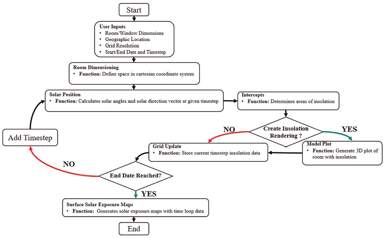
Flowchart structure of program.

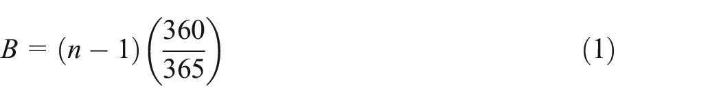
At each timestep the sun’s position is calculated based on the geographic location and time using equation (1) through equation (7) (Blair, 2021). The angular measure, B, accounting for the day number of year, n, is obtained by equation (1).

$$B=(n-1)\left(\frac{360}{365}\right)$$

(1)

$$\mathrm{ET}=229.2\left(\begin{array}{c}0.000075+0.001868\mathrm{cosB}-0.032077\mathrm{sinB}\hfill \\ \multicolumn{1}{c}{-0.014615\cos 2B-0.04089\sin 2B}\end{array}\right)$$

(2)

$$\mathrm{ST}-\mathrm{LST}=4(\mathrm{LSM}-\mathrm{LON})+\mathrm{ET}$$

(3)

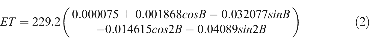
Equations (2) and (3) determine the equation of time in minutes, ET, and the solar time, ST, at the geographic location. Where LST, LSM, and LON are local standard time, local standard meridian and local longitude.

$$\delta =23.45\sin \left(360\frac{284+n}{365}\right)$$

(4)

$${\theta }_z=\mathrm{co}{s}^{-1}(\sin \delta \sin \phi +\cos \delta \cos \omega \cos \phi )$$

(5)

$${\alpha }_s=90-{\theta }_z$$

(6)

$${\gamma }_s=\mathrm{sign}\left(\omega \right)\left|\mathrm{co}{s}^{-1}\left(\frac{\cos {\theta }_z\sin \phi -\sin \delta }{\sin {\theta }_z\cos \phi }\right)\right|$$

(7)

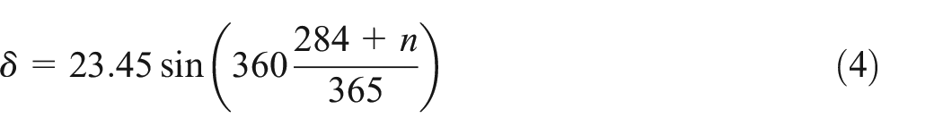
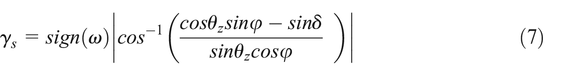
In equations (4)–(7), $\delta$ , ${\theta }_{\mathrm{z}}$ , $\phi$ , $\omega$ , ${\alpha }_{\mathrm{s}}$ , and ${\gamma }_{\mathrm{s}}$ are the declination, zenith angle, latitude, hour angle, solar altitude, and solar azimuth respectively. The term $\mathrm{sign}$ is the positive or negative value of the hour angle.

$${\stackrel{\rightharpoonup }{V}}_{\mathrm{solar}}=[\sin {\theta }_{\mathrm{z}}\sin {\gamma }_{\mathrm{s}},\sin {\theta }_{\mathrm{z}}\cos {\gamma }_{\mathrm{s}},-\cos {\theta }_{\mathrm{z}}]$$

(8)

Utilizing solar angles, the solar direction vector, ${\stackrel{\rightharpoonup }{V}}_{\mathrm{solar}}$ , is determined by equation (8) (Wen and Smith, 2002). Figure 2 illustrates solar angles and the solar direction vector in reference to a cubic space.

$$\mathrm{Ax}+\mathrm{By}+\mathrm{Cz}+D=0$$

(9)

$$[x=x_0+\mathrm{at}][y=y_0+\mathrm{bt}][z=z_0+\mathrm{ct}]$$

(10)

Figure 2.

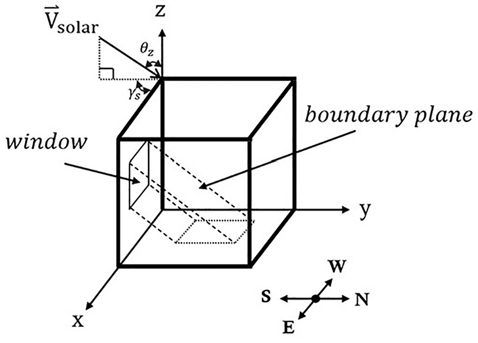
Program geometry.

Following solar direction vector calculation, an iterative process to determine the internal surface areas struck with direct solar radiation is executed utilizing equations (9) and (10) (Wen and Smith, 2002). The process begins by calculating plane equations (equation (9)) for each boundary plane as seen in Figure 2. Plane equations for each window boundary plane are used to calculate x and z intercepts with north wall and are compared to the room bounds to determine insolated surfaces. Using the solar direction vector, arrays of parametric equations for each window corner are calculated (equation (10)). With respective insolated surfaces and plane equations determined, parametric equations are solved and coordinates defining corner bounds of insolated areas are calculated. Bounding line equations between corner bounds are calculated and additional corner bounds are added if multiple surfaces are exposed to insolation. Figure 3 demonstrates the capability of the model to accurately map insolated areas when multiple internal surfaces are struck. Spatial data is stored prior to proceeding to the next timestep.

Figure 3.

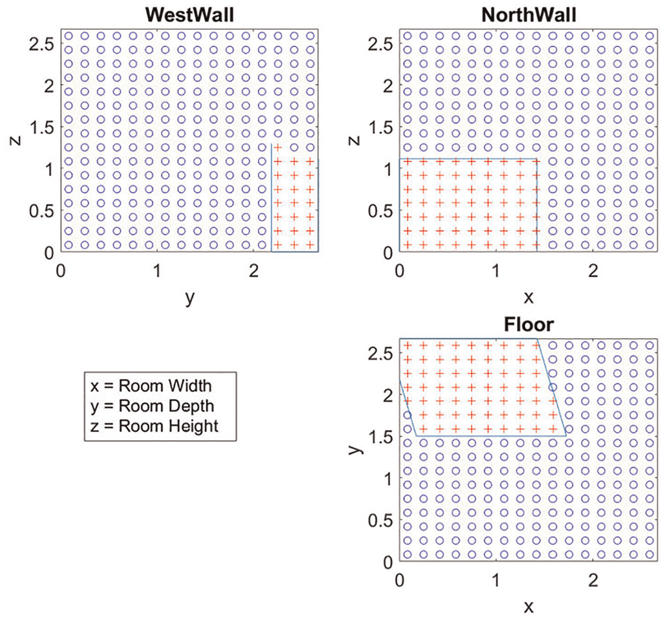
Internal surfaces insolated areas (red plus) distinguished from non-insolated areas (blue circle).

Once the end date is reached, spatial insolation exposure data stored from each timestep over the entire simulation run time is used to generate contour plots. Each contour plot represents one of four internal surfaces (west wall, north wall, east wall, and floor) and displays the spatial exposure of insolation over the user-defined timespan. Areas on surfaces depicted with warmer colors (yellow and orange) represent spots receiving higher durations of the total available insolation while areas depicted with colder colors (dark blue) receive little to no insolation.

Parameters

Model input parameters (envelope dimensions, window dimensions, geographic coordinates) were based on the in-situ chambers located at the Centre for Advanced Building Envelope Research (CABER) in Ottawa, Ontario, Canada. The chamber construction was chosen as results gathered from the MATLAB model are anticipated to guide future full-scale in-situ experiments with passive PCM optimization. Figure 4 depicts the full size in-situ chambers.

Figure 4.

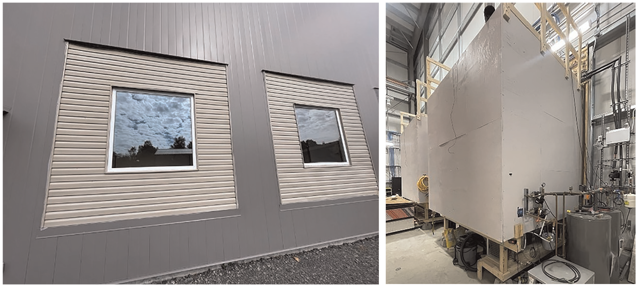
In-situ chambers seen from outside (left) and inside (right).

The time interval, time step and grid resolution are additional input parameters impacting model results. The general objective of the study is to generate insolation exposure maps to determine optimal locations of PCM latent heat storage for full scale experimentation. Because of this, it is important to set time intervals for simulations that represent appropriate periods for PCM optimization. Ottawa, ON is considered a cold climate and experiences two distinct conditioning seasons, both of which are associated with a different temperature setpoint. Winter months typically utilize room heating setpoints of 16°C–21°C while summer months typically utilize room cooling setpoints of 22°C–28°C (Baylis, 2024). An optimized PCM implementation strategy may employ PCMs with melting temperatures and positions tailored to the two distinct room temperature setpoints associated with each conditioning season. Considering this, time intervals for simulations were chosen to represent typical heating and cooling seasons in Ottawa. The exact heating and cooling season of a building may vary significantly depending on various factors such as insulation, size, orientation airtightness, and weather conditions (Abdel-Jaber and Dirks, 2024). Approximated seasons were determined using 1991 to 2020 Canadian climate normals data gathered from the Ottawa airport weather station (Government of Canada, 2024). Cooling and heating season simulations used for insolation exposure map generation ran for periods extending 5.5 and 6.5 months respectively. The applied seasons encompass all periods for which temperatures may drop low enough to require heating or climb high enough to require cooling.

The grid resolution defines the number of rows and columns used when distributing uniform grid points on surfaces. A grid resolution of 100 uniformly distributes 10,000 grid points across each surface. The timestep defines how frequently calculations determining solar exposure bounds across surfaces are updated. Prior evaluation revealed shorter timesteps require higher grid resolutions to accurately depict contours on insolation exposure maps and significantly increase simulation run time as iterative processes are increased. Because lower grid resolutions have larger separations between grid points, small changes in insolation boundaries that occur with smaller timesteps may not be detected. Longer timesteps did not require a higher grid resolution to produce insolation exposure maps and decreased simulation run times. To limit simulation run times running over entire conditioning seasons a grid resolution of 6 points per meter (depicted in Figure 3) and a timestep of 1 hour was deemed acceptable.

Model assessment

To assess the accuracy of the solar ray tracing method employed in the MATLAB model, a single room model of the in-situ chamber was developed in ESP-r and compared. The insolation tool invoked by the user in ESP-r provides solar altitude, solar azimuth, and internal surface radiance proportion data with 1-h timesteps for a singular day of each month in a year. The same monthly days were input and ran in the MATLAB program. June 11th, March 16th, and December 11th were chosen for comparison of the two models to ensure agreement of solar data across the bounds of an annual solar profile. Figure 5 provides visuals of the insolation rendering agreement between the two models.

Figure 5.

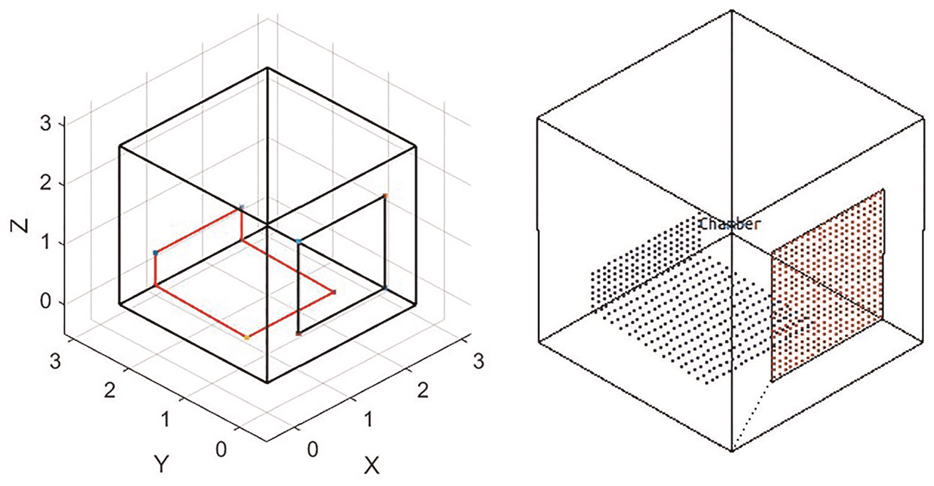
MATLAB (left) and ESP-r (right) insolation rendering of in-situ chamber on February 15th at 13:00.

To make a direct comparison an additional script was added into the MATLAB program to calculate and store solar insolation data at each hour of the day in a similar manner to the ESP-r model. Solar azimuth and solar altitude angles between the two models tended to be in strong agreement when compared directly. Slight differences in solar angles were limited to 1° difference and notably caused by rounding differences between equations used in the two models. Figures 6 and 7 display a direct comparison between the two models for the proportion of insolation received on the Floor and East wall, respectively. As shown in Figure 6, the models reflect corresponding distributions. From sunrise to solar noon the proportion of insolation hitting the floor increases and from solar noon to sunset the proportion decreases. On the comparison day in December the MATLAB model attributed a proportion of insolation exposure to the north wall that was 14.5% less on average during the total 5 hours of exposure than the Esp-r model. The exact gridding resolution used in ESP-r is not provided and the difference in resolution between the two models was attributed to this difference. With varying grid resolutions, one model might over attribute proportional area to a surface while the other under attributes the proportional area.

Figure 6.

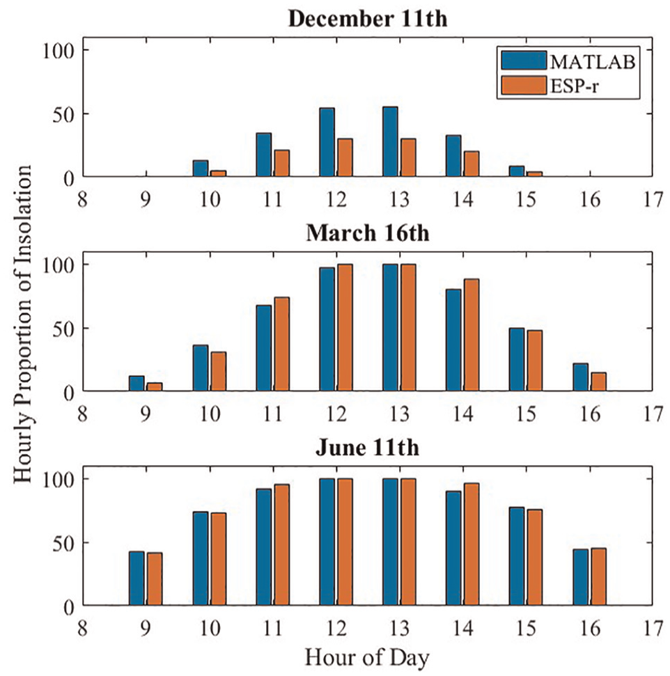
ESP-r and MATLAB model comparison of hourly insolation proportions received on the floor on June 11th, March 16th, and December 11th.

Figure 7.

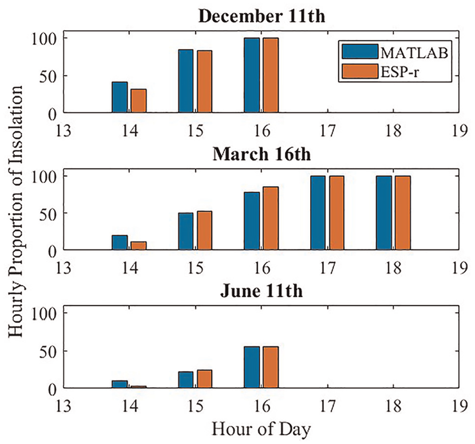
ESP-r and MATLAB model comparison of hourly insolation proportions received on the east wall on June 11th, March 16th, and December 11th.

In Figure 7, a similar distribution can be seen on the east wall for all 3 days assessed. The proportion of solar radiation received increases as the day advances from solar noon to sunset with both models. For the day in December, a higher proportion of insolation is attributed to the east wall due to the solar altitude being lower. On the contrary, the east wall receives a significantly lower proportion of sunlight in June due to two factors: a higher solar altitude during the midday hours causes most of the direct solar radiation to hit the floor, and the solar azimuth passes 90°W before the solar altitude decreases, thus preventing any direct solar radiation from entering the room. These trends are representative of what occurred on the north wall and west wall. The west wall exhibited the inverse trend of the east wall showing the highest attributed proportion of direct solar radiation at sunrise and decreasing till solar noon. The north wall exhibited the same trend throughout the day as the floor for October through February and received no direct irradiance from March through September.

By summing the hourly insolation proportions for each internal surface, the daily insolation proportions can be determined as demonstrated in Figure 8. This calculation demonstrates the total time proportion of direct solar radiation striking each surface across a day which shows the correlation between the two models. Both models show similar proportions across each surface for June 11th and March 16th. However, on December 11th differences of 10.9% and 12.6% exist between models for the floor and the north wall when calculating daily insolation proportions. Visual renderings of both models were examined on this date and found to depict similar insolation distributions. Due to the limited capabilities of the ESP-r insolation tool the exact cause could not be pinpointed, but the difference in grid resolutions used between the two models is likely to be one factor.

Figure 8.

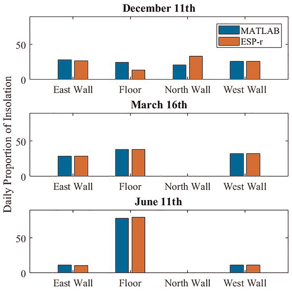
ESP-r and MATLAB model comparison of daily average insolation proportions received on all internal surfaces on June 11th, March 16th, and December 11th.

The MATLAB model developed was deemed to agree with the ESP-r model due to the similar predictions across all cases of comparison. Despite the slight difference in proportions attributed to the north wall and floor during the singular day in December, it is expected that this difference would be reduced over a larger simulation runtime. This is because each day the insolation path on the internal surfaces shifts slightly. Thus, the impact of outlier days is reduced when a proportional average is taken over longer simulation periods. Following assessment of the MATLAB model with the ESP-r model, the MATLAB model was then used for the duration of the study to develop insolation exposure maps that were generated and evaluated for distinct conditioning season in the year.

Results

Heating season

Figure 9 shows the summed insolation exposure maps generated by the MATLAB model of the in-situ chambers located in Ottawa with a runtime set from October 15th through May 1st. Each internal surface is mapped to its location in a 2D template for easier data visualization. The east and west walls exhibit similar levels of insolation exposure while the north wall exhibits the lowest level and the floor the highest. The ellipse area on the floor may receive a maximum of 580 h of insolation exposure over the general heating season which equates to an average of 3 h per day, while areas outlined in dark blue exhibit no exposure.

Figure 9.

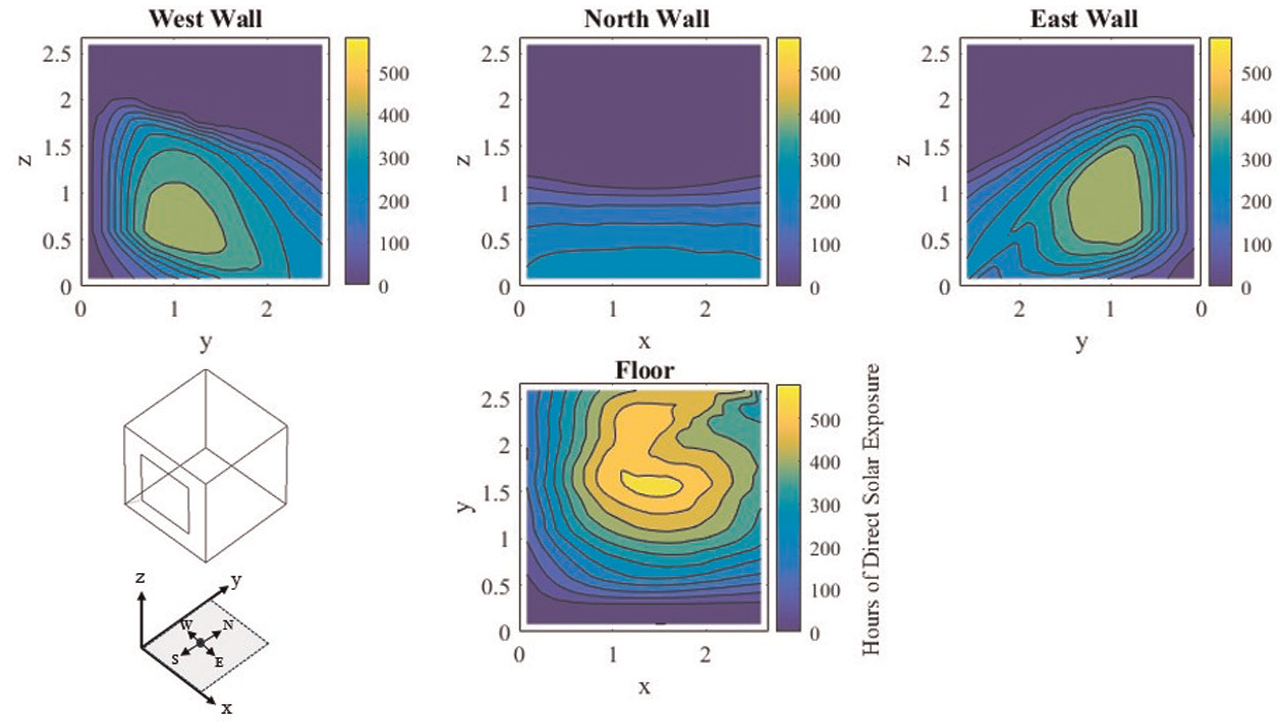
Insolation exposure maps generated for a typical Ottawa heating season – October 15th to May 1st.

On October 15th the areas of insolation exposure in the room are more southerly. As time progresses toward winter solstice on December 21st, the solar altitude decreases, and the solar azimuth becomes more southerly during daylight hours. This in turn causes the areas of direct insolation exposure to creep north day by day on the floor, east wall, and west wall. On December 21st, the north wall receives its largest proportion of insolation. As time then progresses past winter solstice to the end of the heating season on May 1st, the days get longer, the solar altitude increases during daylight hours and the solar azimuth stretches to the east and west.

Previous comparison chart data in Figure 8 may indicate that the east and west walls receive their largest proportion of direct insolation during the equinoxes. However, these graphs do not consider the area that is incident on a surface. For example, on March 16th 100% of the insolation is incident on the east wall for two consecutive hours in the evening. During this time the solar azimuth is greater than +70° and approaches +90°. As the solar azimuth becomes more westerly, the projected window area through which direct solar radiation can pass is significantly reduced. This effect is also prevalent with solar altitude. As the position of the sun in the sky increases, the perceived area of the window decreases. Thus, as time approaches the equinoxes, the daily measurable time in which the east and west walls are exposed to insolation increases while the area of exposure on each wall is significantly reduced. The insolation exposure maps were compared for each month, and it was observed that the east and west walls have a higher exposure during the months closer to winter solstice.

Cooling season

Figure 10 shows the insolation exposure maps generated from May 1st until October 15th. Compared to Figure 9, it is seen that the east and west walls display the same trend with a slight difference in insolation exposure levels. This is caused by the 1-h timestep slightly favoring exposure to the east wall over the west wall with respect to sunrise and sunset times. Further analysis of Figure 10 reveals most of the insolation exposure in the room is localized to the southern half of the floor which receives a maximum of 600 h of insolation exposure. On the contrary, the east, west, and north walls receive significantly lower levels.

Figure 10.

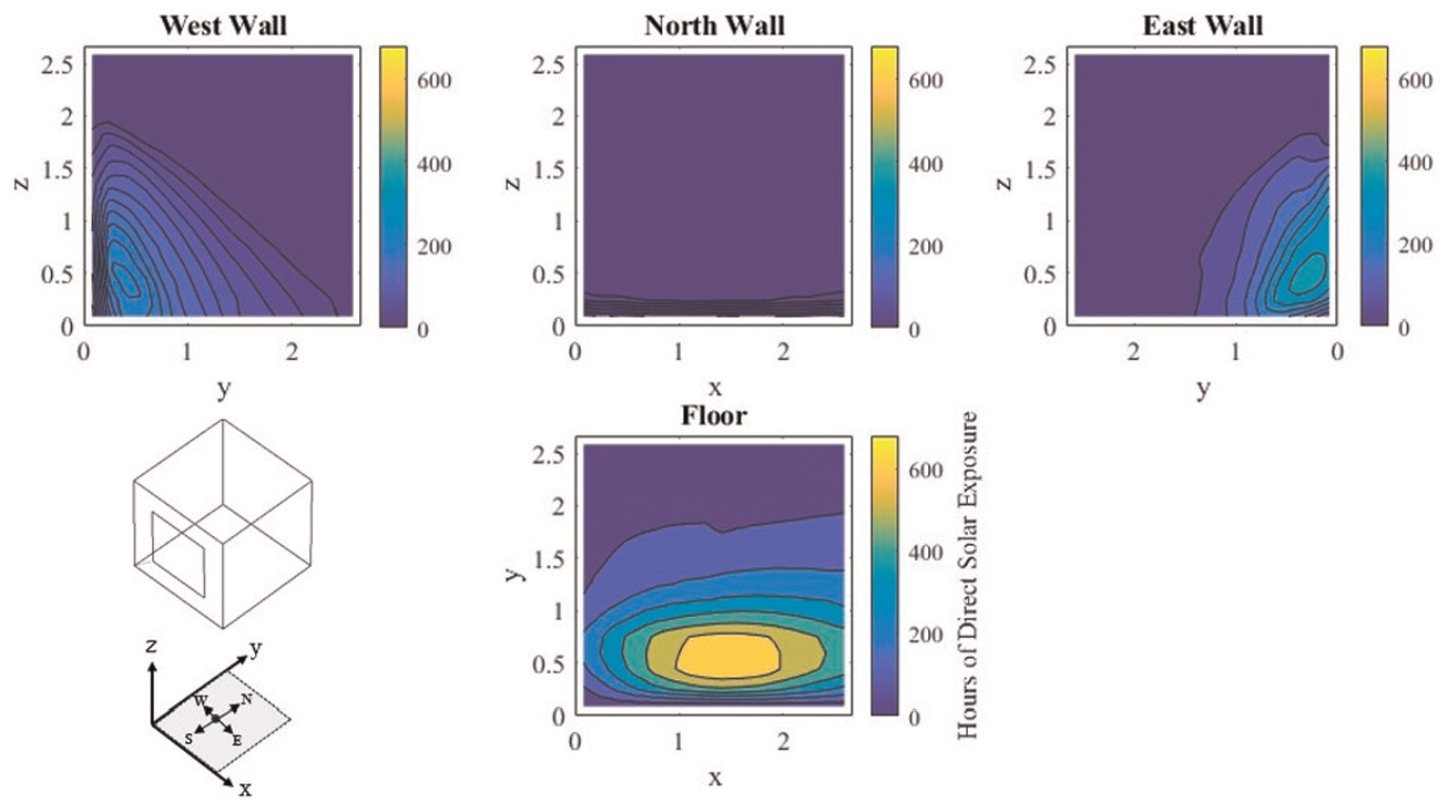
Insolation exposure maps generated for a typical Ottawa cooling season – May 1st to October 15th.

On May 1st, the areas of insolation exposure in the room are more northerly. As time progresses toward the summer solstice, the sun’s altitude increases, and the solar azimuth extends west and east during daylight hours. This causes the areas of insolation exposure to creep south each day on the floor, west wall, and east wall. Afterwards, from summer solstice till the end of the cooling season simulation on October 15th, areas of insolation creep north each day. The north wall does not receive any insolation until the final few days of the simulation period.

During the cooling season the east and west walls receive significantly lower levels of insolation exposure compared to the heating season. This is due to two main reasons. The first is that the room is only subjected to a south facing window and direct solar radiation can only enter the room when the solar azimuth is within the −90° (east) and +90° (west) bounds. The second reason is that when the solar altitude is low enough in the morning and evening for favorable wall insolation conditions the solar azimuth is too far to the east or west, only allowing a sliver of direct solar radiation to pass through the south facing window.

A month-by-month analysis of insolation exposure levels on the floor revealed that months between the spring and fall equinox produced the highest insolation exposure levels. This was expected as the solar altitude during daylight hours over these months is much greater causing a higher portion of the insolation to hit the floor rather than side walls. As the solar altitude increases to its maximum of 69.5° on the summer solstice the power density of the direct solar radiation on the floor increases while the receiving area decreases.

Annual analysis

Based on the data gathered from the insolation exposure maps, the total proportion of insolation exposure per surface for each distinct conditioning season was charted as seen in Figure 11. This comparison shows that the floor has the highest exposure to insolation in both conditioning seasons. During the heating and cooling season, it receives 70% and 43% of the total exposure respectively. As such, it is predicted that an optimized latent heat storage system would integrate PCM into the floors for increased thermal storage due to insolation.

Figure 11.

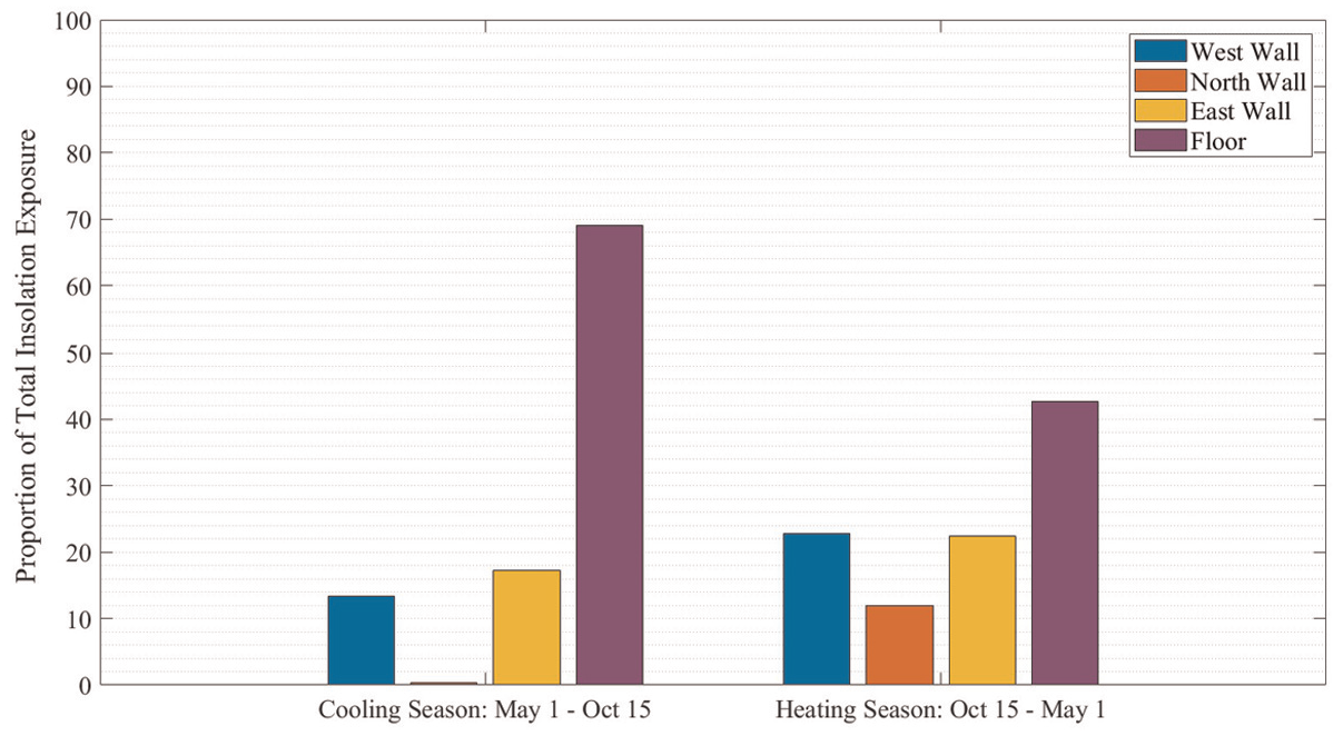
Proportional irradiance exposure of internal surfaces during distinct conditioning seasons.

The direct comparison between the east wall and west wall shows similar exposure proportions between the two surfaces due to the symmetry of the in-situ model. Comparing these surfaces between conditioning seasons, the walls receive a higher proportion of insolation exposure during the heating season. This is due to the lower solar altitude in the winter months in the northern hemisphere. Finally, the north wall receives a negligible proportion of insolation exposure over the cooling season and the lowest proportion over the heating season. For the in-situ chambers it is not suggested to integrate PCM into this surface due to its reduced exposure to insolation over the course of a year.

Model limitations and assumptions

Through the development of the MATLAB program, it is recognized that assumptions were made which limit the insolation data produced. The first being that the program produced insolation exposure maps as a function of area and time omitting the intensity of the insolation. The intensity of insolation depends on the angle between the incoming sunlight and the surface on which it strikes. Insolation has its highest power density when perpendicular to an incident surface. As the incident angle decreases from 90° the power density associated with the insolation decreases. Building off the current program, a subfunction should be incorporated which considers the intensity of the insolation on each surface based on the incident angle between the solar direction vector and the incident plane. Furthermore, the insolation maps generated could be a function of exposure area, time, and intensity.

As the objective of the study was to determine the total insolation availability, the program assumes uniform sky transparency each day. This assumption omits cloud coverage which would reflect and scatter sunlight reducing the insolation exposure on internal surfaces. Since the program quantifies insolation as a measurement of time availability rather than energy, the energy absorbed by each surface from direct radiation could not be quantified. As a result of this, less energy intense forms of radiation that would also be absorbed by wall surfaces such as diffuse and ground reflected were not included.

Conclusions and future work

The objective of this study was to develop a model capable of providing a deeper analysis into insolation exposure on surfaces compared to current BPS tools and realize ideal locations for spatially optimized passive PCM systems. The comparisons undertaken with ESP-r confirmed program accuracy. The MATLAB model produced insolation proportions that were on average within 7.3% of ESP-r insolation proportions for all surfaces. A larger difference was noted in the proportion of insolation received by the north wall and floor during the December comparison. This difference was caused by the difference in grid resolutions between the two models. The insolation intensity maps generated for the heating and cooling seasons revealed that the northern half and southern half of the floor are exposed to the highest levels of insolation during the heating season and cooling season respectively, receiving 3–4 h of solar exposure on average per day. This indicates that it may be beneficial to implement PCMs into distinct northern and southern regions of the floor to maximize latent heat storage and reduce peak room temperatures during distinct conditioning seasons.

This study provides an in-depth analysis on insolation exposure within spaces, allowing for future optimization of latent heat storage and reduction in PCM implementation costs. It is important to note that the results acquired in this study pertain to the modelled building space in Ottawa, ON and that the results produced by the model will vary depending on room dimensions, window sizes, geographic locations, and climatic conditions. Considering these results, significant additional research is suggested to further prove optimization strategies of latent heat storage systems in the real world. A full-scale experiment integrating PCM into floor materials of the chambers should be undertaken to examine the potential increased benefits of localizing PCM to areas of higher insolation exposure. These experiments should take place to quantify the spatially optimized performance of PCM in practice. It is also suggested that a future study utilizes inputs available to the user to conduct a larger analysis. Within this scope, room parameters and geographical locations may be varied to assess their impact on generated insolation maps for respective heating and cooling seasons and draw trends between spatial optimization within different geographic locations and geometries.