Sage Journals: Discover world-class research

Abstract

The widespread advancement of computer technology resulted in the increasing usage of deep learning models for predicting solar radiation. Numerous studies have been conducted to explore their research potential. Nevertheless, the application of deep learning models in optimizing building energy systems, particularly in a multi-step solar radiation prediction model for model predictive control (MPC), remains a challenging task. This is mainly due to the intricacy of the time series and the possibility of accumulating errors in multistep forecasts. In this study, we propose the development of a transformer-based attention model for predicting multi-step solar irradiation at least 24 h in advance. The model is trained and tested using measured solar irradiation data and temperature forecast data obtained from the Tokyo Meteorological Agency. The findings indicate that the transformer model has the capability to effectively mitigate the issue of error accumulation. Additionally, the generative model exhibits a significant improvement in accuracy, with a 62.35% increase when compared to the conventional regression LSTM model. Additionally, the transformer model has been shown to attain superior prediction stability, mitigate the effects of error accumulation in multi-step forecasting, and circumvent training challenges stemming from gradient propagation issues that can occur with recurrent neural networks.

Keywords

Solar radiation multi-step prediction time series data deep learning interpretable deep learning

Introduction and background

Background

With the rapid expansion of the global economy and the concurrent rise in urbanization, an increasing proportion of people’s daily lives is spent in indoor environments, such as commercial or residential buildings. In fact, research has shown that people now spend over 80% of their time inside such structures, which highlights the critical role that buildings play in shaping human experiences and health (Wang et al., 2018). The contemporary trend of urbanization and the growing global economy have resulted in a significant surge in the amount of time individual spend inside buildings. As a consequence, there has been a substantial upsurge in building energy consumption in recent times. Research shows that by 2021, building energy consumption has accounted for up to 40% of the total energy consumption of the entire society, encompassing both residential and commercial buildings (Grillone et al., 2021). The energy consumption associated with buildings contributes significantly to global CO2 emissions. This is primarily due to the extensive use of primary energy sources in building energy systems. In fact, the greenhouse gas emissions attributed to buildings constitute approximately 30% of the total global emissions (Gao et al., 2022a). Due to the significant demand for reducing carbon emissions, there has been a growing focus on integrating renewable energy sources with building energy systems. This coupling has become a natural consideration in efforts to reduce carbon footprints and promote sustainable energy practices.

Achieving the objective of emission reduction requires a crucial coupling of building energy systems with renewable energy sources, as emphasized by previous research (Pinamonti and Baggio, 2020). Solar energy is a crucial and well-established form of renewable energy. As a result, its integration into building energy systems has become an increasingly vital strategy for reducing building energy consumption (Gao et al., 2022b). However, the integration of renewable energy sources into building energy systems has presented significant challenges in terms of control and optimization. The unpredictability of renewable energy output, in particular, poses a major obstacle to the eﬀicient and effective management of building energy systems (Gao et al., 2022c). As a result, ensuring the stability of system power generation and eﬀiciently dispatching large-scale equipment, such as power generators, pose significant challenges. This is highlighted by previous research (van der Meer et al., 2018). The eﬀicient operation of building systems can lead to effective energy conservation and reduced emissions (Qian et al., 2019).

In the given context, Model Predictive Control (MPC) has garnered significant attention as a promising technology that can eﬀiciently attain desired objectives (Gao et al., 2023). The precise prediction of solar irradiation is crucial in optimizing the management of both the entire system and the power grid. This can facilitate a more eﬀicient integration of solar energy and building energy systems, leading to significant energy savings and reduced emissions (Sharma et al., 2011).

Machine learning and deep learning methods for solar irradiation prediction

Solar irradiation is generally correlated with various meteorological parameters, including but not limited to pressure, temperature, wind speed, relative humidity, and sunshine duration. The strength of these correlations can vary depending on factors such as geographic location and time of year. One frequently employed approach is to establish a regression model for forecasting by utilizing the meteorological parameters of a specific location (Zhang et al., 2017). In the earlier stages of research, solar radiation (irradiation) prediction in the field commonly employed mature statistical models and machine learning algorithms (Nidhul et al., 2023).

However, the effective utilization of statistical models and machine learning algorithms is contingent upon a thorough comprehension of solar irradiation datasets as well as the intricate process of feature engineering (Khodayar et al., 2017). Furthermore, it is noteworthy that the aforementioned method may exhibit inadequate processing power when it comes to handling high-dimensional features (Ahmad et al., 2018). Given the aforementioned limitations, there has been an increasing utilization of deep learning models for solar irradiation prediction (Kumari and Toshniwal, 2021). Recurrent neural networks, such as LSTM (Long short-term memory) (Gao et al., 2020), have gained popularity as the preferred choice for deep learning models, owing to their unique structure specifically designed for processing sequential data.

For instance, Kaba et al. (2018) employed deep learning techniques to predict and validate data from over 30 solar radiation measurement stations in Turkey. The proposed model yielded a high coeﬀicient of determination of 0.98, indicating its ability to accurately predict solar radiation levels. Sun et al. (2019) successfully predicted short-term solar radiation at 15-min intervals, achieving a remarkably low root mean squared error (RMSE) of 2.1 kW, as reported in their study. Qing and Niu (2018) utilized Long Short-Term Memory (LSTM) to forecast the solar radiation for the following day on an hourly basis. Their findings indicated that the predicted Root Mean Squared Error (RMSE) of the LSTM model was 42.9% lower than that of an Artificial Neural Network (ANN).

Based on the findings presented, it is evident that the deep learning model demonstrates a robust ability to fit single-step solar radiation (irradiation) prediction. Moreover, the model exhibits superior predictive performance in comparison to other methods in several cases, particularly when compared to the LSTM model.

Multi-step solar radiation prediction

While previous research has largely focused on predicting solar radiation at a single time step in the future, the application scenarios for an MPC optimization model require a solar irradiation prediction model capable of forecasting multiple time steps ahead. Thus, it is necessary to develop and evaluate prediction models that can meet the specific requirements of the MPC optimization model. Taking into account various factors, such as equipment safety, peak and valley electricity prices, and other relevant variables, it is common for the forecast window to extend up to 1 week or more, as evidenced by several studies (Ceusters et al., 2021). In general, multi-step ahead prediction techniques commonly comprise of four distinct strategies: the direct strategy (DS), the recursive strategy (RS), as well as a combination of both via the combined direct and recursive strategy (DRS). The technique of dynamic sampling (DS) effectively simplifies the prediction process by converting multi-step ahead forecasts into single-step predictions. This method utilizes multiple models to accurately forecast time series data that contain varying time intervals between observations (Tran et al., 2009). However, the establishment of numerous models contributes significantly to the complexity of the model (Sorjamaa et al., 2007). Additionally, it should be noted that in many cases, the time series of different time steps are assumed to be independent and the time dependency is disregarded (Lu et al., 2021).

The RS method is characterized by a straightforward single-step prediction process, which distinguishes it from the DS method. Unlike the DS method, the RS approach does not require the establishment of multiple models. Rather, it utilizes the predicted value of the model as the input to forecast the subsequent solar radiation, as documented In and Jung (2022). The use of predictions as input, rather than measured values, in the modeling process can lead to an increase in the prediction error (Ahani et al., 2020). One example of using machine learning techniques for solar radiation prediction is found in the work of Guermoui et al. (2018). In their study, they employed the Gaussian regression process to forecast solar radiation for 1–10 future time steps. Their findings suggest that as the prediction range increases, the accuracy of the model decreases.

To address the issue of error accumulation, it is imperative to implement a specialized design for the model structure. Qing and Niu (2018) employed Long Short-Term Memory (LSTM) to develop a structured output solar irradiation prediction model. The authors drew inspiration from the sequence-to-sequence approach used in natural language processing (Sutskever et al., 2014) to address the issue of error accumulation caused by repeated input of predicted values. The model’s output comprises a 24-length vector, effectively resolving this issue. Although the seq2seq model has been widely utilized in multi-step ahead prediction to solve issues with time dependence, it suffers from certain limitations, such as the inability to handle long-term dependencies. Specifically, the conventional sequence-to-sequence LSTM model, also known as seq2seq-LSTM, may encounter issues with long-distance dependence. Additionally, as the length of the sequence increases, the accuracy of the model’s predictions may decrease significantly, as noted in previous studies (Li et al., 2021).

Research gap and objective

Based on the preceding discussion of related work, the authors posit that there are several areas that represent a research gap in solar irradiation prediction models applied to MPC. Specifically, the error accumulation is believed to require further investigation in this paper.

When researchers attempt to apply the existing one-step regression model to multi-step forecasting, they may encounter the issue of error accumulation, as supported by numerous studies in the literature (see Figure 1). This simple application may not suﬀice for accurate forecasting, and it is crucial for researchers to consider alternative models or approaches that can better handle multi-step forecasting scenarios. As the prediction step progresses, it may require the model to calculate the output of the previous step in order to generate a prediction for the next moment. This process can introduce additional errors into the model, which may compound as the number of iteration steps increases. Despite the importance of multi-step prediction in many applications, the literature survey revealed that only a limited number of studies have been specifically designed to address this challenge.

Figure 1.

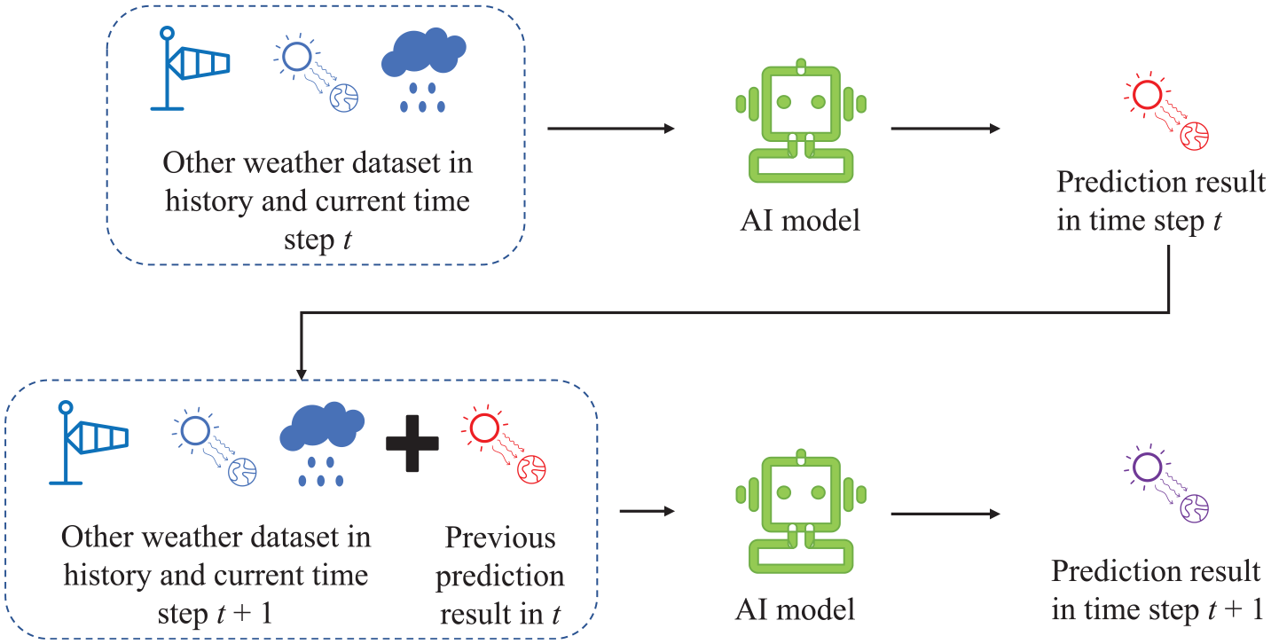
Error accumulation when using single step regression model (Gao et al., 2022a).

In order to address the limitations of traditional multi-step prediction methods, which may result in the loss of temporal dependencies between predicted solar radiation values and long-distance information in seq2seq models, this study explores the effectiveness of a transformer model for multi-step ahead prediction. Specifically, the study employs historical hourly data from the previous days to forecast hourly solar radiation values for the following day. By doing so, this approach seeks to improve the accuracy and reliability of radiation predictions which maybe used in MPC framework.

Method

Data preprocessing

In the realm of machine learning algorithms, data preprocessing, also known as feature engineering, plays a critical role in the entire process. While the emergence of deep learning has reduced the significance of feature engineering to a considerable extent, the variance in the input feature values can still have a significant impact on the weight of the features during model training. As a result, it is imperative to normalize the features even in deep learning processes, as highlighted by previous research (Goodfellow et al., 2016).

This paper explores the use of three normalization methods, namely z-score, log normalization, and one-hot code, for different features and labels.

The z-score normalization method is a commonly used approach in data preprocessing. It involves transforming data to have a mean of zero and a standard deviation of one. The formula for z-score normalization is as follows (equation (1)):

\hat{x} = \frac{x - μ}{σ}

(1)

where µ is the mean of all of the characteristics, σ indicates the standard deviation of the mean, and xˆ is the result of standardizing.

In time-series forecasting, the statistical properties such as mean and variance of a time series are likely to vary across different time periods. Consequently, the data used in training and testing of the model may not follow the same distribution. When dealing with stable weather parameters, the z-score method is a reasonable choice. However, for building energy consumption data, which may exhibit significant variations over time due to social development, log standardization is a preferred preprocessing technique, as recommended by previous studies (Kodama et al., 2016).

The process of log normalization can be mathematically represented by the following equation (equation (2)):

z = lo g_{a} x

(2)

where x is the raw data, and z is the result of log standardizing.

Attention

The origins of the attention mechanism can be traced back to the field of machine translation, where it was first proposed in its earliest form (Bahdanau et al., 2014). In the context of machine translation, an attention mechanism is employed to facilitate word alignment and ensure the accuracy of the language model. The word alignment problem in machine translation is often mitigated using an attention mechanism, which is known to improve the accuracy of the language model. In the context of time-series forecasting, this mechanism can be extended to the field of solar radiation forecasting, provided that the Query (Q), Key (K), and Value (V) are appropriately defined. To illustrate this, a computational schematic of the attention mechanism is presented in Figure 2.

α_{i} = softmax (s (K_{i}, Q))

(3)

Attention = \sum_{i = 1}^{N} α_{i} V_{i}

(4)

Figure 2.

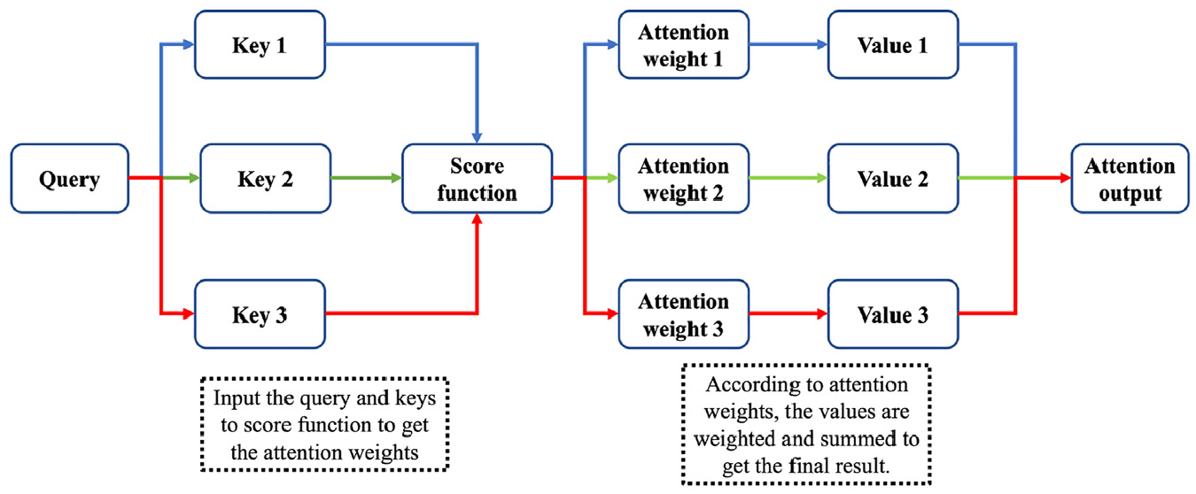
Attention calculation process (Gao and Ruan, 2021).

To calculate the attention mechanism, one can follow these steps:

To calculate the attention weight, we input the Q vector and different K vectors individually into the score function, as illustrated in equation (3). Here, the variable s represents the attention score function. It is worth noting that the definitions of score functions can vary significantly, ranging from a straightforward vector dot product to a more complex neural network architecture. The softmax function, as described by LeCun et al. (2015) in the context of deep learning, is utilized to transform the output of the score function into a probability distribution33. In this study, the Q vector refers to the pertinent information related to the prediction target, such as the date and time, among other factors that have an impact on the subsequent moment. The K vector, on the other hand, denotes the relevant information in the historical data. The number of K vectors is typically equal to the length of the encoded data. For instance, if we utilize 168 h of historical data to forecast 1 h into the future, we will have a total of 168 K vectors. Similar to the concept of a query, the aim is to identify information that bears greater resemblance to the target being predicted, in order to produce a conclusive outcome.

Once the attention weights have been acquired, the final attention calculation result can be obtained by taking the weighted sum of the V vector and the weights, as shown in equation (4). This process is referred to as the attention value calculation.

Transformer

Since the proposal of the attention mechanism, it has gained widespread usage when combined with a Recurrent Neural Network (RNN), as has been shown in Ruiz et al.’s (2016) study. Despite the identification of the relationship among sequence data, RNNs require iterative and sequential calculations, which negatively impact computational eﬀiciency. Additionally, as computing power advances, longer sequences are being processed by networks, further exacerbating the challenge posed by the primitive nature of sequence data processing. This has led to significant obstacles in the actual computing process. In 2017, Google introduced a transformer model that utilizes a self-attention mechanism (Vaswani et al., 2017). The Transformer model employs self-attention, which overcomes the issues of iterative calculation and long sequence forgetting that are present in RNN networks. By leveraging the benefits of parallel computing, the Transformer model enhances operational speed while providing a significant improvement in interpretability through its attention mechanism.

The calculation method for the transfer method varies between the encoder and decoder. The specific workflow for each process is illustrated in Figure 3.

Figure 3.

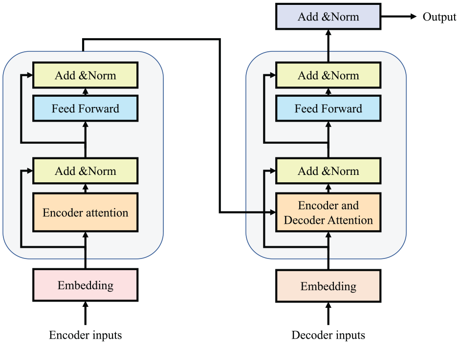
Workflow of transformer.

The transformer architecture maintains the conventional structure of an encoder and decoder model, as outlined by Cho et al. (2014). Initially, the input data is passed through the embedding layer, where it is processed for information and latitude. In the encoder, self-attention is commonly employed for computation. This involves using the same vectors for the Query, Key, and Value in attention calculation. Figure 4 illustrates the concept of self-attention.

Figure 4.

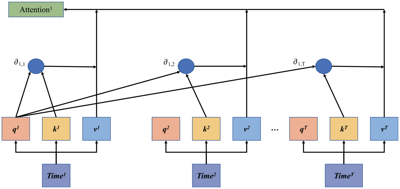
Workflow of self-attention.

Figure 4 illustrates an example of how the attention value of the first time step is calculated. To begin, each time step’s information is first embedded and duplicated into three identical vectors: q, k, and v. Here, T represents the length of the entire time-series data. For instance, if we encode 168 h of historical data, then T would be 168.

When calculating the attention value at the initial moment, the vector at that moment becomes the query. As the network needs to comprehend the relationship between different time steps within the time series, the Key vector comprises the information of all time steps in the current time series. Moreover, as the final attention value is expected to reflect the relationship between the current time step and the time series, the Value vector also includes the input time-series information.

Evaluation methods

To rigorously assess the predictive performance of the model, several evaluation indices are utilized. The primary metrics employed include Mean Absolute Error (MAE) and Coeﬀicient of Determination (R2). The mathematical representations of these indices are provided below:

MAE = \frac{1}{N} \sum_{i = 1}^{N} | \hat{y} - y |

(5)

R^{2} = 1 - \frac{\sum_{i = 1}^{i} {(\hat{y} - y)}^{2}}{\sum_{i = 1}^{N} {(μ_{y} - y)}^{2}}

(6)

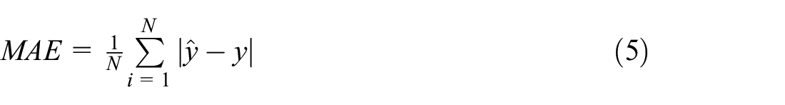
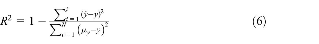
Among equation (5) to equation (6), N represents the number of calculation samples, $\hat{y}$ and y demonstrate the real measured data and the predicted data, $μ_{y}$ means the mean value of actual data.

Case study

Introduction of dataset

The data utilized in this study was collected and released by the Japan Meteorological Agency (JMA), which reports weather data and forecasts throughout Japan. Specifically, this paper utilizes a real measured dataset collected around Tokyo Station. The dataset spans from January 1, 2019 at 0:00 to December 31, 2020 at 23:00, providing 2 years of hourly data. Solar irradiation and temperature data measured at various points were primarily used by the authors.

The dataset comprises primarily of three distinct components of data:

The self-built features comprise of five distinct features: day of year, week of year, month, hour, and sun rise. Day of year, week of year, and month signify the changes in position of different data points throughout the year. These features have been artificially constructed to aid in forecasting since the solar irradiation intensity varies considerably across different seasons and months. The hour and sun rise features, on the other hand, represent the positional and change characteristics of hourly data in a day. The “sunrise” feature to some extent substitutes the information conveyed by solar elevation and azimuth angles. The relationship between solar irradiation data and the rise and fall of the sun is inseparable. Hence, these two features can help the model better determine whether solar irradiation is present at the current prediction step and how strong its intensity is.

The dataset comprises 10 numerical features, namely: land pressure (hPa), sea pressure (hPa), penetration (mm), temperature (°C), dew temperature (°C), water vapor pressure (hPa), humidity, wind speed (m/s), radiation time (h), and cloud cover. These features were measured hourly, collected, and sorted by the measuring equipment of the Japan Meteorological Agency. This is real measured features.

The weather forecast data used in this study includes the oﬀicial daily temperature forecast data, specifically, the maximum and minimum daily temperature, issued by the JMA. This is using to simulate the real weather forecasting. Since we’re using real values, we’ll get slightly better results than using the weather forecast.

Lastly, regarding the solar radiation label: in the original dataset, the unit of measurement is MJ/m², representing the solar radiation energy received per hour. However, in line with conventional practices in solar radiation forecasting, we’ve assumed uniform radiation over the hour and thus converted the energy unit to a power unit.

Experimental setup

Definition of models

To facilitate a comprehensive analysis of the generative model employed in this article and the impact of weather forecast on irradiation prediction, the authors have devised various models to ascertain the eﬀicacy of the methods.

M.1: This model utilizes a Long Short-Term Memory (LSTM) network in conjunction with a regression model to forecast solar irradiation. The LSTM network encodes the current length sequence and subsequently predicts the solar irradiation values for the next time step. Furthermore, while the transformer model can generate multi-step prediction results by sampling all at once, the M.1 model is limited to outputting predictions for one future time step at a time. However, in order to achieve the objective of multi-step prediction, the M.1 model utilizes an iterative forecasting method for future solar irradiation forecasting.

M.2: M.2 Use the transformer model proposed in this paper to directly perform multi-step prediction. In the encoder, we utilize all available features and labels to effectively encode and learn from the data. Our encoding process involved 168 h of data. Subsequently, in the decoder phase, we input specific known parameters, such as time characteristics and weather forecasts, to simulate maximum and minimum temperatures. The decoder then directly decodes for a period of 24 h. We aim to leverage the transformer model to mitigate error accumulation by enabling direct output, thereby improving the accuracy of multi-step predictions.

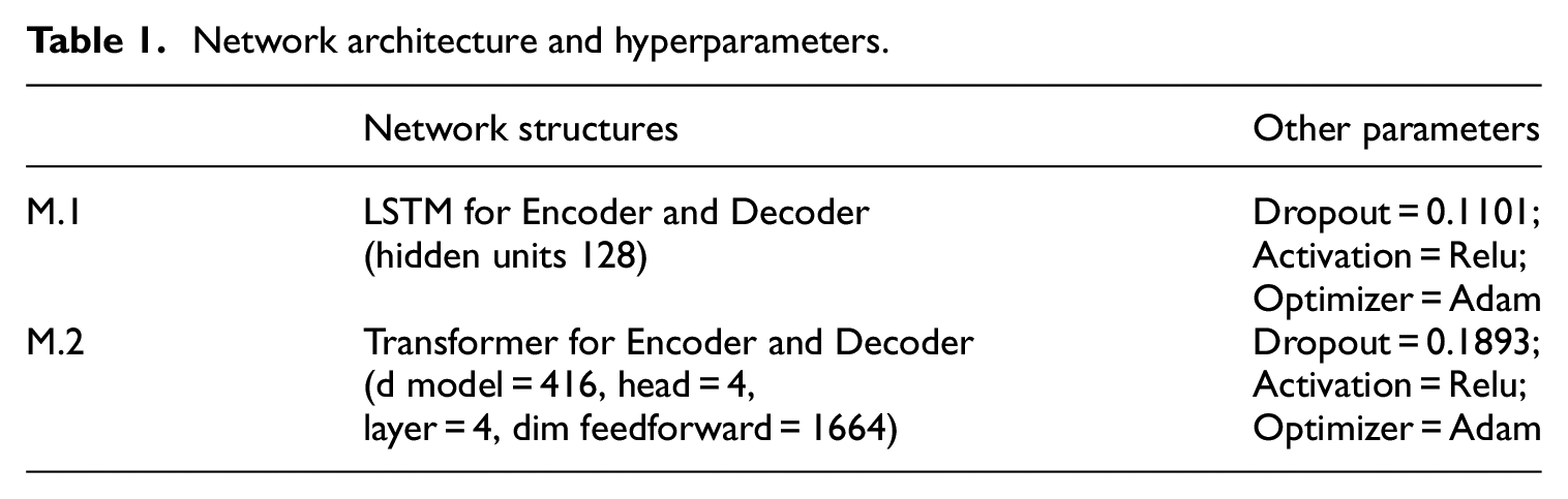
The models were developed and implemented using Python 3.7 and Pytorch 1.9. Our aim with the generative model M.2 was to address the issue of error accumulation caused by iterative prediction, which the regression model M.1 employs. Through our experimentation, we anticipate that M.2 will outperform M.1 when working with identical data inputs. It was observed that the coding length of the LSTM and transformer model amounted to 168 h, which implies that we have incorporated the weekly periodicity of the time series data. Additionally, the model’s ability to learn and account for time dependencies relies on various factors, including the day of the year, week of the year, month, hour, and so on, which possess distinctive characteristics. Table 1 presents the hyperparameter configurations of the model. All hyperparameters were optimized within a fixed range and step size using Optuna (Akiba et al., 2019), with a consistent random seed to ensure experiment stability.

Table 1.

Network architecture and hyperparameters.

	Network structures	Other parameters
M.1	LSTM for Encoder and Decoder(hidden units 128)	Dropout = 0.1101; Activation = Relu; Optimizer = Adam
M.2	Transformer for Encoder and Decoder(d model = 416, head = 4,layer = 4, dim feedforward = 1664)	Dropout = 0.1893; Activation = Relu; Optimizer = Adam

In this study, the dataset was partitioned based on a time period, and the same methodology was employed for all models. The dataset consisted of 24 months of data over a period of 2 years, and it was divided into 24 equal parts, with a training set, validation set, and test set ratio of approximately 6:2:2 (Géron, 2022).

Specifically, the training set consisted of data from January 2019 to March 2020, which was used to train the model. This decision was made to ensure that the training data encompasses a complete year, which is crucial for learning the annual variation of solar radiation. The validation set, comprising data from April 2020 to July 2020, was used to fine-tune the model and obtain optimal results using Optuna. Finally, the test set was used to generate the model’s predictions, and any differences were subsequently analyzed and discussed from August 2020 to December 2020.

Results and discussion

The statistical results of the two models utilized in the experiment are presented in Table 2. It’s important to note that we converted all solar radiation units to kW/m² for the analysis of results.

Table 2.

Evaluation metric used in the predictions.

	MAE in total (kW/m²)	R2
M.1	265.26	53.83%
M.2	146.57	87.40%

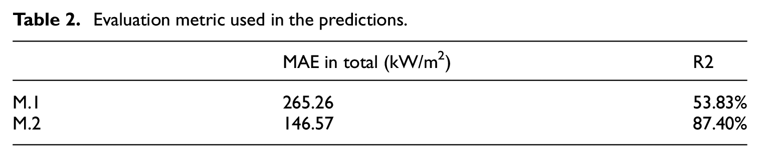
The performance of M.2 demonstrates a marked improvement over the traditional iterative regression M.1, with a 53.83% increase in the R2 score. Notably, M.2 attains a high R2 score of 0.8740, indicating a robust regression fit. When considering the overall absolute error of the dataset, M.2 showed a decrease from approximately 265.26 to 146.57, indicating an increase of 44.74% compared to M.1. The M.2 model has shown significant improvement, as evidenced by its R2 fitting degree of 0.874 and comparison with the results obtained from the M.1 model. The performance of M.1 in terms of prediction results is notably subpar, which can be attributed to the accumulation of errors. This finding provides compelling evidence for the necessity of our proposed M.2 model structure.

Furthermore, Figure 5 depicts a histogram plot illustrating the distribution of prediction errors at each time step. It should be noted that the solar irradiation data contains numerous zero values, corresponding to times when the sun sets. Therefore, the figure only includes time steps where the solar irradiation value is non-zero.

Figure 5.

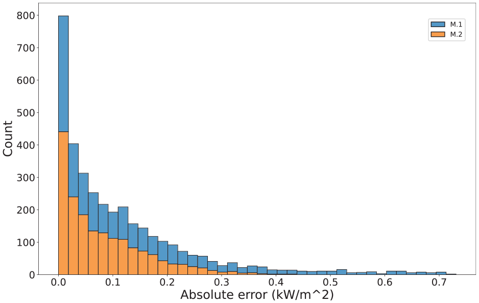
Histogram of M.1 and M.2 prediction results.

The findings indicate that the M.2 model generates fewer outlier predictions compared to the regression model, thereby demonstrating greater stability in its prediction results. The authors suggest that the transformer model mitigates the accumulation of errors resulting from repeated use of the prediction outcomes, leading to more reliable results. Such enhanced stability is particularly beneficial for final application scenarios, including model predictive control (MPC), as it promotes more rational optimization outcomes. To provide readers with a more intuitive understanding of the model’s predictive performance, a selection of test set results has been presented in the form of a line graph (Figure 6). This enables readers to visualize the impact of the model’s predictions more clearly. The use of transformer models still exerts a significant influence on the prediction outcomes, as can be inferred from the visualization presented.

Figure 6.

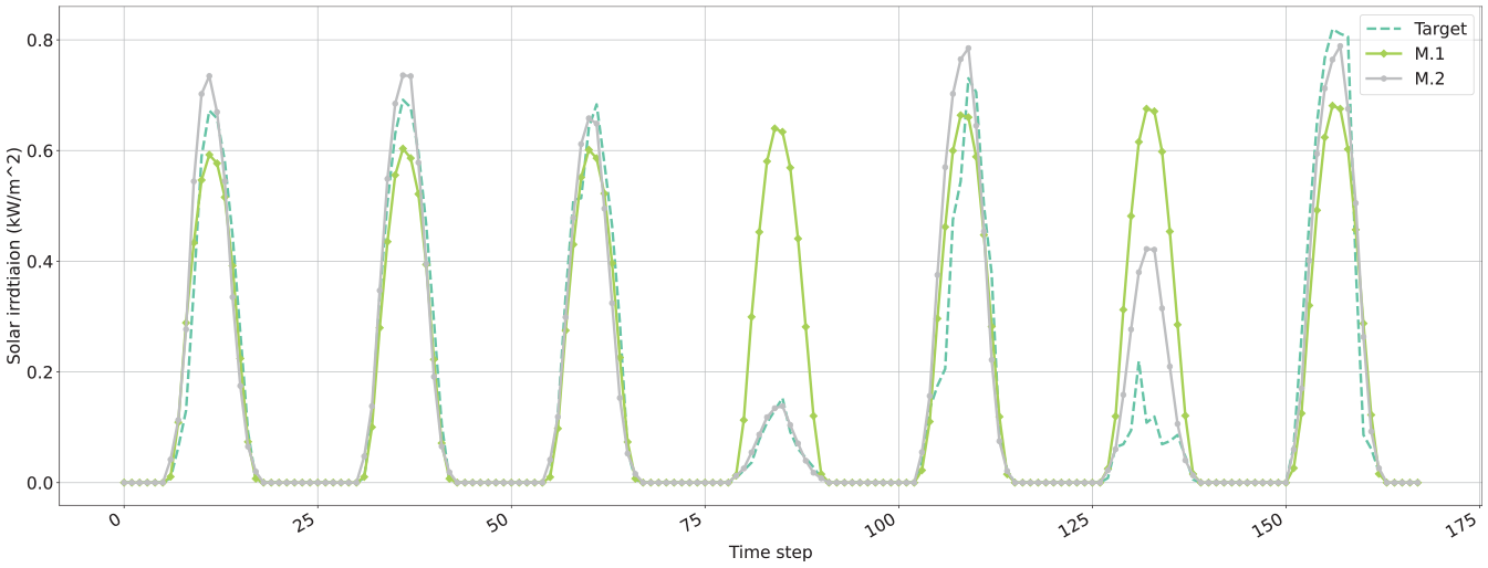
Visualization of forecast results.

Specifically, the data obtained on the fourth day reveals a marked reduction in solar irradiation, and it is at this juncture that M.2 outperforms other models in accurately forecasting the peak solar irradiation for the day. This observation holds immense relevance for equipment scheduling in MPC applications.

Finally, MAE at various hours of the day is analyzed and plotted for both August and December, as represented in Figures 7 and 8. The error magnitude corresponds to the point size in the scatter plot. The error pattern largely parallels the daily solar radiation trend, with greater errors occurring around noon when solar radiation peaks. Furthermore, the prediction accuracy for December surpasses that of August. This is because the absolute value of solar radiation in summer is greater than that in winter. The results from August and December exhibit a similar pattern, wherein higher solar radiation corresponds to greater generated error. However, within this daily distribution, the M.2 model outperforms M.1, particularly during the peak solar radiation hours around noon.

Figure 7.

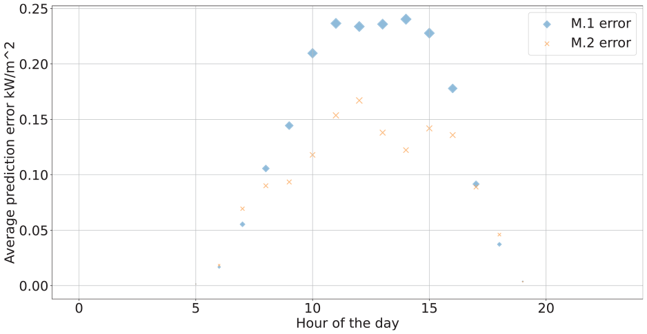
Hourly average MAE in August.

Figure 8.

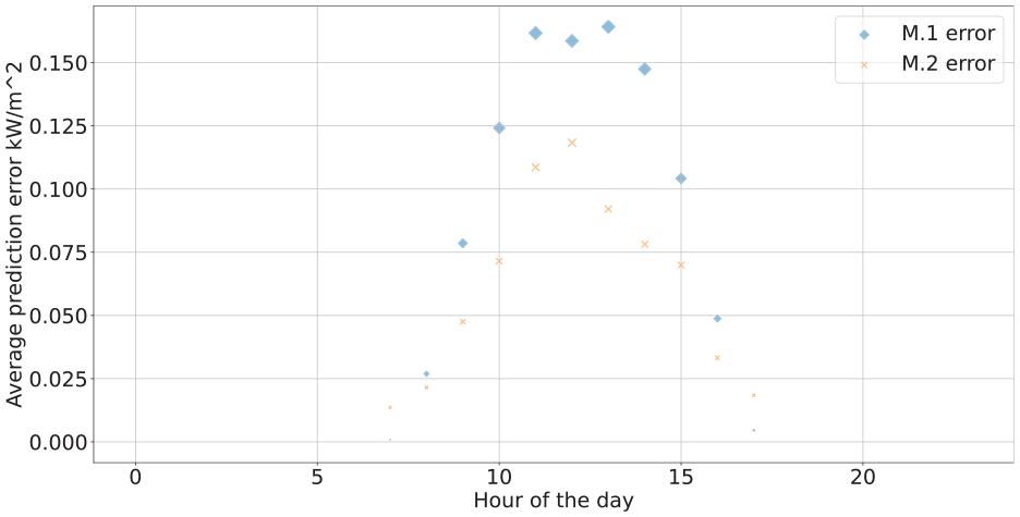
Hourly average MAE in December.

Conclusions and future work

Multi-step prediction of solar radiation is crucial for the operational optimization of renewable energy systems. This paper proposes a transformer-based multi-step solar radiation prediction model. Using the characteristics of the transformer avoids the problem of gradient descent caused by iterative calculations in the RNN network. At the same time, it also avoids the accumulation of errors caused by repeated predictions using the single-step model. The following conclusions can be drawn.

The transformer model based on the attention mechanism is better at capturing long-distance dependencies. It overcomes the time dependence problem of the output sequence which is diﬀicult to be considered by traditional multi-step look-ahead forecasting models. It also represents a new approach to multi-step-ahead forecasting.

Compared with the single-step LSTM model used iteratively, the proposed transformer model has achieved a 62.35% improvement in R2 fit, and the overall prediction is also more problematic.

The transformer model has been demonstrated to outperform conventional multi-step-ahead time series forecasting models in terms of both forecast accuracy and stability. In addition to its successful use in solar radiation forecasting, this model can also be applied to forecasting in other fields and applications, including wind energy forecasting, building energy forecasting, and inventory change forecasting. However, while the transformer model can capture global features by discarding the inherent structure of RNN, it may not capture local features as effectively. Thus, a combination of RNN and transformer models may lead to improved prediction results, particularly by capturing both local and global features.

Footnotes

Declaration of conflicting interests

The author(s) declared no potential conflicts of interest with respect to the research, authorship, and/or publication of this article.

Funding

The author(s) received no financial support for the research, authorship, and/or publication of this article.

ORCID iD

Pengwei Tang

References

Ahani

Salari

Shadman

(2020) An ensemble multi-step-ahead forecasting system for fine particulate matter in urban areas. Journal of Cleaner Production 263: 120983.

Ahmad

Mourshed

Rezgui

(2018) Tree-based ensemble methods for predicting PV power generation and their comparison with support vector regression. Energy 164: 465–474.

Akiba

Sano

Yanase

, et al. (2019) Optuna: A next-generation hyperparameter optimization framework. In: Proceedings of the 25th ACM SIGKDD international conference on knowledge discovery & data mining, pp.2623–2631. ACM.

Bahdanau

Cho

Bengio

(2014) Neural machine translation by jointly learning to align and translate. arXiv preprint arXiv:1409.0473.

Ceusters

Rodríguez

García

, et al. (2021) Model-predictive control and reinforcement learning in multi-energy system case studies. Applied Energy 303: 117634.

Cho

Van Merriënboer

Gulcehre

, et al. (2014) Learning phrase representations using rnn encoder- decoder for statistical machine translation. arXiv preprint arXiv:1406.1078.

Gao

Miyata

Akashi

(2022b) Interpretable deep learning models for hourly solar radiation prediction based on graph neural network and attention. Applied Energy 321: 119288.

Gao

Miyata

Akashi

(2022c) Multi-step solar irradiation prediction based on weather forecast and generative deep learning model. Renewable Energy 188: 637–650.

Gao

Matsunami

Miyata

, et al. (2022a) Multi-agent reinforcement learning dealing with hybrid action spaces: A case study for off-grid oriented renewable building energy system. Applied Energy 326: 120021.

10.

Gao

Matsunami

Miyata

, et al. (2023) Model predictive control of a building renewable energy system based on a long short-term hybrid model. Sustainable Cities and Society89: 104317.

11.

Gao

Ruan

(2021) Interpretable deep learning model for building energy consumption prediction based on attention mechanism. Energy and Buildings 252: 111379.

12.

Gao

Ruan

Fang

, et al. (2020) Deep learning and transfer learning models of energy consumption forecasting for a building with poor information data. Energy and Buildings223: 110156.

13.

Géron

(2022) Hands-on Machine Learning With Scikit-Learn, Keras, and Tensor Flow. Sebastopol, CA: O’Reilly Media, Inc.

14.

Goodfellow

Bengio

Courville

(2016) Deep Learning. Cambridge, MA: MIT Press.

15.

Grillone

Mor

Danov

, et al. (2021) A data-driven methodology for enhanced measurement and verification of energy efficiency savings in commercial buildings. Applied Energy301: 117502.

16.

Guermoui

Melgani

Danilo

(2018) Multi-step ahead forecasting of daily global and direct solar radiation: A review and case study of Ghardaia region. Journal of Cleaner Production 201: 716–734.

17.

Jung

J-Y

(2022) Simple averaging of direct and recursive forecasts via partial pooling using machine learning. International Journal of Forecasting 38(4): 1386–1399.

18.

Kaba

Sarıgül

Avcı

, et al. (2018) Estimation of daily global solar radiation using deep learning model. Energy 162: 126–135.

19.

Khodayar

Kaynak

Khodayar

(2017) Rough deep neural architecture for short-term wind speed forecasting. IEEE Transactions on Industrial Informatics 13(6): 2770–2779.

20.

Kodama

Okabe

Kogiso

(2016) Simultaneous estimation of contraction ratio and parameter of mckibben pneumatic artificial muscle model using log-normalized unscented kalman filter. In: 2016 IEEE 4th international conference on cyber-physical systems, networks, and applications (CP- SNA), pp.44–48. New York: IEEE.

21.

Kumari

Toshniwal

(2021) Deep learning models for solar irradiance forecasting: A comprehensive review. Journal of Cleaner Production318: 128566.

22.

LeCun

Bengio

Hinton

(2015) Deep learning. Nature 521(7553): 436–444.

23.

Xiao

Zhang

, et al. (2021) Attention-based interpretable neural network for building cooling load prediction. Applied Energy299: 117238.

24.

Tian

Zhou

, et al. (2021) Multi-step-ahead prediction of thermal load in regional energy system using deep learning method. Energy and Buildings233: 110658.

25.

Nidhul

Thummar

Yadav

, et al. (2023) Machine learning approach for optimization and performance prediction of triangular duct solar air heater: A comprehensive review. Solar Energy 255: 396–415.

26.

Pinamonti

Baggio

(2020) Energy and economic optimization of solar-assisted heat pump systems with storage technologies for heating and cooling in residential buildings. Renewable Energy 157: 90–99.

27.

Qian

Niu

, et al. (2019) Nationwide savings analysis of energy conservation measures in buildings. Energy Conversion and Management 188: 1–18.

28.

Qing

Niu

(2018) Hourly day-ahead solar irradiance prediction using weather forecasts by lstm. Energy 148: 461–468.

29.

Ruiz

Cuéllar

Calvo-Flores

, et al. (2016) An application of non-linear autoregressive neural networks to predict energy consumption in public buildings. Energies 9(9): 684.

30.

Sharma

Irwin

, et al. (2011) Predicting solar generation from weather forecasts using machine learning. In: 2011 IEEE international conference on smart grid communications (SmartGridComm), pp.528–533. New York, NY: IEEE.

31.

Sorjamaa

Hao

Reyhani

, et al. (2007) Methodology for long-term prediction of time series. Neurocomputing 70(16–18): 2861–2869.

32.

Sun

Venugopal

Brandt

(2019) Short-term solar power forecast with deep learning: Exploring optimal input and output configuration. Solar Energy 188: 730–741.

33.

Sutskever

Vinyals

(2014) Sequence to sequence learning with neural networks, Advances in neural information processing systems 27.

34.

Tran

Yang

Tan

ACC

(2009) Multi-step ahead direct prediction for the machine condition prognosis using regression trees and neuro-fuzzy systems. Expert Systems with Applications 36(5): 9378–9387.

35.

van der Meer

Widén

Munkhammar

(2018) Review on probabilistic forecasting of photovoltaic power production and electricity consumption. Renewable and Sustainable Energy Reviews 81: 1484–1512.

36.

Vaswani

Shazeer

Parmar

, et al. (2017) Attention is all you need. Advances in neural information processing systems 30.

37.

Wang

Zeng

, et al. (2018) Random forest based hourly building energy prediction. Energy and Buildings 171: 11–25.

38.

Zhang

Zhao

Deng

, et al. (2017) A critical review of the models used to estimate solar radiation. Renewable and Sustainable Energy Reviews 70: 314–329.

Multi-step solar radiation prediction using transformer: A case study from solar radiation data in Tokyo

Abstract

Keywords

Introduction and background

Background

Machine learning and deep learning methods for solar irradiation prediction

Multi-step solar radiation prediction

Research gap and objective

Method

Data preprocessing

Attention

Transformer

Evaluation methods

Case study

Introduction of dataset

Experimental setup

Definition of models

Results and discussion

Conclusions and future work

Footnotes

Declaration of conflicting interests

Funding

ORCID iD

References