Sage Journals: Discover world-class research

Abstract

The analysis of heat, air, and moisture (H.A.M.) transport for building envelopes are known to be highly dependent on climate loads and air infiltration rates. Moisture content within the assembly is often a key H.A.M. analysis outcome to assess risk and transport behavior. ASHRAE Standard 160-2016 states that building envelope H.A.M. analysis should be done using moisture design reference data or using a minimum of 10 consecutive years of weather. While there has been progress and methods for selecting or designing moisture reference years there has been a lack of study in the impact of multi-year (particularly 10-year) weather scenarios on simulation results in comparison to reference year simulations. This paper presents research using stochastic 1, 2, and 10-year weather data and air infiltration rates to study the range of simulated moisture content outcomes for four wall assemblies in Philadelphia and compares these to the outcomes when using reference years. Results from the study show that air infiltration, starting month, and multi-year duration have significant impacts on simulated moisture content, mold, and corrosion analysis results. Regression analysis using annual averages of climate input parameters did not yield useable models for selecting weather years, however an estimated mold index value using outdoor climate data may be useful in selecting weather years with varying starting months for mold growth assessment.

Keywords

Hygrothermal air infiltration stochastic multi-year mold moisture

Introduction

Building envelope economic context

Buildings, along with their design, construction, use, and maintenance are considerable financial investments that have long term impact on our energy use, human health, and productivity. In 2018 building construction in the United States accounted for $840 billion of GDP (U.S. Bureau of Economic Analysis, 2019). In 2020 building sector energy consumption was approximately one-third of total energy expenditures globally (González-Torres et al., 2022). Building envelopes have a significant impact on the thermal performance and energy use of buildings. Space conditioning and lighting is estimated to be 18% of overall residential and commercial building energy use (DOE, 2015). As building envelopes directly impact heating, cooling, and lighting, the design, use, and maintenance of building envelopes can influence building energy consumption and carbon emissions. Thus, the performance of the building envelope is a critical asset that deserves careful design and evaluation.

Building envelopes are typically designed to be cost effective, durable with an expectation to last decades, provide thermal and moisture protection from the outside, and require minimal maintenance. Building envelope failures are often due to moisture related damage, such as staining, decay, mold growth, corrosion, delamination, and geometric movement (Brambilla and Sangiorgio, 2020; Chitte and Sonawane, 2018; Zabel and Morrell, 2012; Zelinka, 2013). Each of these can occur due to prolonged elevated moisture content within building envelope materials. In addition to moisture related material damage, high moisture content in the building envelope has been linked to negative respiratory health due to poor indoor air quality. The economic cost of asthma treatments due to elevated moisture in buildings is estimated at $3.5 billion in the US (Mudarri and Fisk, 2007).

Stochastic methods, uncertainty, and sensitivity analysis of building envelopes

In professional practice in the United States most long-term assessment of moisture within building envelopes utilize criteria such as those prescribed by ASHRAE Standard 160: Criteria for Moisture-Control Design Analysis in Buildings (ASHRAE, 2016) and numerical simulations as described by EN15026 Hygrothermal performance of building components and building elements – Assessment of moisture transfer by numerical simulation (EN 15026, 2007). In recent years there has been a greater awareness in the research community of the need for assessing building envelope risks probabilistically and to include uncertainty and sensitivity analysis with the assessment of building envelopes (Janssen, 2013; Prada et al., 2014; Tian, 2013; Tian et al., 2018). This is particularly relevant as building envelope simulations often rely on complex models based on many parameters that may have a high degree of uncertainty. Identifying which parameters to focus on for higher quality or better fitting data can significantly influence simulation results. For example, researchers studying heat flux through building envelopes in Argentina, utilized multivariate statistical techniques to determine the most significant meteorological variables in predicting thermal performance of vertical opaque envelopes (Thomas et al., 2022). Multiple linear regression analysis showed that outdoor air temperature and solar irradiance were the most important meteorological variables for heat flux in their studied cases.

Using envelope hygrothermal analysis researchers have examined probabilistic mold growth and biodeterioration of wood in buildings and demonstrated that variations in climate conditions significantly impact mold growth and deterioration (Sadovský et al., 2014; Vereecken et al., 2015). Others have studied the hygrothermal performance of highly insulated wood framed walls using stochastic modeling and concluded that for the studied assemblies, uncertainties of material properties did not result in significant simulated results for moisture content and mold growth. Instead they found that the uncertainties of moisture loads (such as air infiltration) had significant impact on the outcomes and were related to climate conditions (Wang and Ge, 2018).

Looking at a large range of previous research Gradeci and Berardi examined probabilistic approaches for evaluating building envelopes to withstand mold growth. They noted 21 papers within their literature review evaluating building envelope performance (1997–2018) using probabilistic methods. The vast majority of these used a single year either based on a reference year, moisture design reference year, random sample, or severe year. Some used periods less than a year and only four studies used multi-year durations for simulations. They stated that the outdoor climate is the most important parameter and that when accounted for wind-driven rain penetration can significantly increase mold growth in their study case (Gradeci and Berardi, 2019).

Numerical simulation of building envelopes has become more widely used in assessing envelope designs, and recent research shows that uncertainty is a strong area of research interest (di Giuseppe et al., 2017; Hagentoft et al., 2015; Wang et al., 2021). Many of the above-mentioned studies noted that variations and uncertainty in climate data can lead to large variations in simulated outcomes. Currently the widely accepted standard in the United States for envelope moisture analysis, ASHRAE Standard 160-2016 states that analysis “shall be performed using a minimum of 10 consecutive years of weather data or using the moisture design reference years weather data” (ASHRAE, 2016). As seen in the Gradeci and Beradi’s findings, the vast majority of envelope analyzes lack multi-year weather scenarios in favor of moisture reference years. Like structural design methods, most envelope moisture assessments rely on checking for failure at extreme conditions, meaning that envelopes designs are simulated against a limited set of worst-case weather scenarios, often referred to as moisture reference years. Simulating envelopes may involve using worst case scenarios such as a very hot and humid weather year, a particularly cold year, and/or a year with especially heavy rainfall (Salonvaara et al., 2011). Envelope simulations using moisture reference years make the implicit assumption that the envelope will experience the highest moisture content under these worst-case 1-year scenarios rather than testing envelopes across a probabilistic range of scenarios or across longer multi-year scenarios. While climate and material parameters have been studied in previous research, stochastic 10-year weather coupled with stochastic air infiltration, has not been well studied in hygrothermal envelope analysis and their study should benefit the building science community.

Limitations of existing methods

ASHRAE Standard 160-2016 provides direction on many of the needed hygrothermal design parameters and ASHRAE RP-1325 augments the moisture-design reference years to be selected using a damage function. However, the criterion of using 10 consecutive years of weather data is not well defined in comparison to the moisture-design reference years. As performing a 10-year simulation is more computational expensive and without knowing which 10-years to use, it may be that in practice most hygrothermal simulations are performed using reference years and not 10-year weather data. Given that moisture accumulation and mold growth are both time dependent outcomes, single reference weather years may underpredict moisture levels when compared with simulations using 10-years of weather data. In terms of air infiltration rates, which impact building energy and envelope moisture behavior, it is known that in North America there is a wide range of infiltration rates (Persily et al., 2010) in both existing and new construction and most buildings are not tested during construction to verify airtightness. Using 0.1 and 0.2 air changes per hour as the air infiltration rate could be a mischaracterization and the use of a range of probabilistic air infiltration rates may be beneficial.

Research objective

This paper hypothesizes that envelope hygrothermal simulations using single-year single trial moisture reference years for weather may underestimate moisture content and related moisture damage when compared to simulations using stochastic multi-year (2- and 10-year weather data) and probabilistic air infiltration rates.

The remainder of this paper is organized in three main sections. “Methodology”, presents the methodology used in the research. “Results and discussion”, presents and discusses the results of the project. Comparisons of the moisture outcomes, including mold and corrosion risk, for simulations done with reference years and multi-year trials are made. In “Summary” conclusions are given.

Methodology

This project studied the variation in building envelope moisture outcomes when simulated using historic multi-year weather (2- and 10-year) data and compared the range of outcomes to those produced when using moisture reference years (1- and 2-year periods). After initial studies showed considerable moisture content at the start of the simulation period the project scope increased to include varying the starting month of 2-year simulation periods. Lastly the project also probabilistically varied infiltration rates.

The project used an augmented version of HAM-Tools detailed in previous publication (Chung et al., 2020) to facilitate wind-driven rain, rain penetration, stochastic inputs, H.A.M. simulation, predict moisture content, mold growth, and corrosion within common ventilated envelope assemblies. Since HAM-Tools is an open source H.A.M. analysis tool, its Simulink model and Matlab code was augmented to include mold growth and corrosion risk analysis based on criteria detailed in ASHRAE Standard 160-2016. The general workflow of inputs, analysis, and outputs can be seen in Figure 1.

Figure 1.

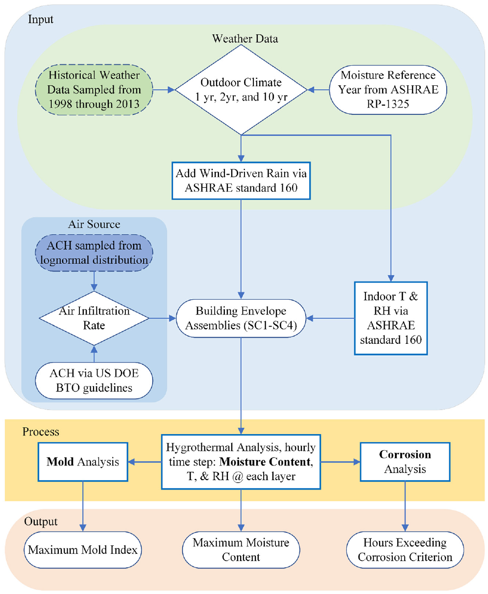
Schematic diagram of workflow. See Table 1 for list of assemblies. Dashed lines denote sampled inputs.

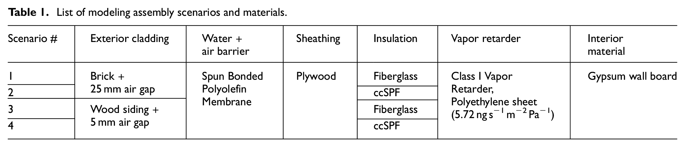
Wood framed building envelopes are the most common building envelope type used in residential construction in the United States (Jellen and Memari, 2019). Ventilated claddings are the most typical contemporary exterior surface treatment for framed wall assemblies (Bradtmueller and Foley, 2014). This project utilized guidelines published by the United State Department of Energy Building Technology Office (US DOEBTO) for simulating ventilated claddings to predict moisture content levels within typical exterior walls (Lstiburek et al., 2016). The list of the assemblies studied is shown in Table 1 and uses the same assemblies as previously reported (Chung et al., 2020). The location of the simulations is Philadelphia, Pennsylvania, USA.

Table 1.

List of modeling assembly scenarios and materials.

Scenario #	Exterior cladding	Water + air barrier	Sheathing	Insulation	Vapor retarder	Interior material
1	Brick + 25 mm air gap	Spun Bonded Polyolefin Membrane	Plywood	Fiberglass	Class I Vapor Retarder, Polyethylene sheet (5.72 ng s⁻¹ m⁻² Pa⁻¹)	Gypsum wall board
2	Brick + 25 mm air gap			ccSPF
3	Wood siding + 5 mm air gap			Fiberglass
4	Wood siding + 5 mm air gap			ccSPF

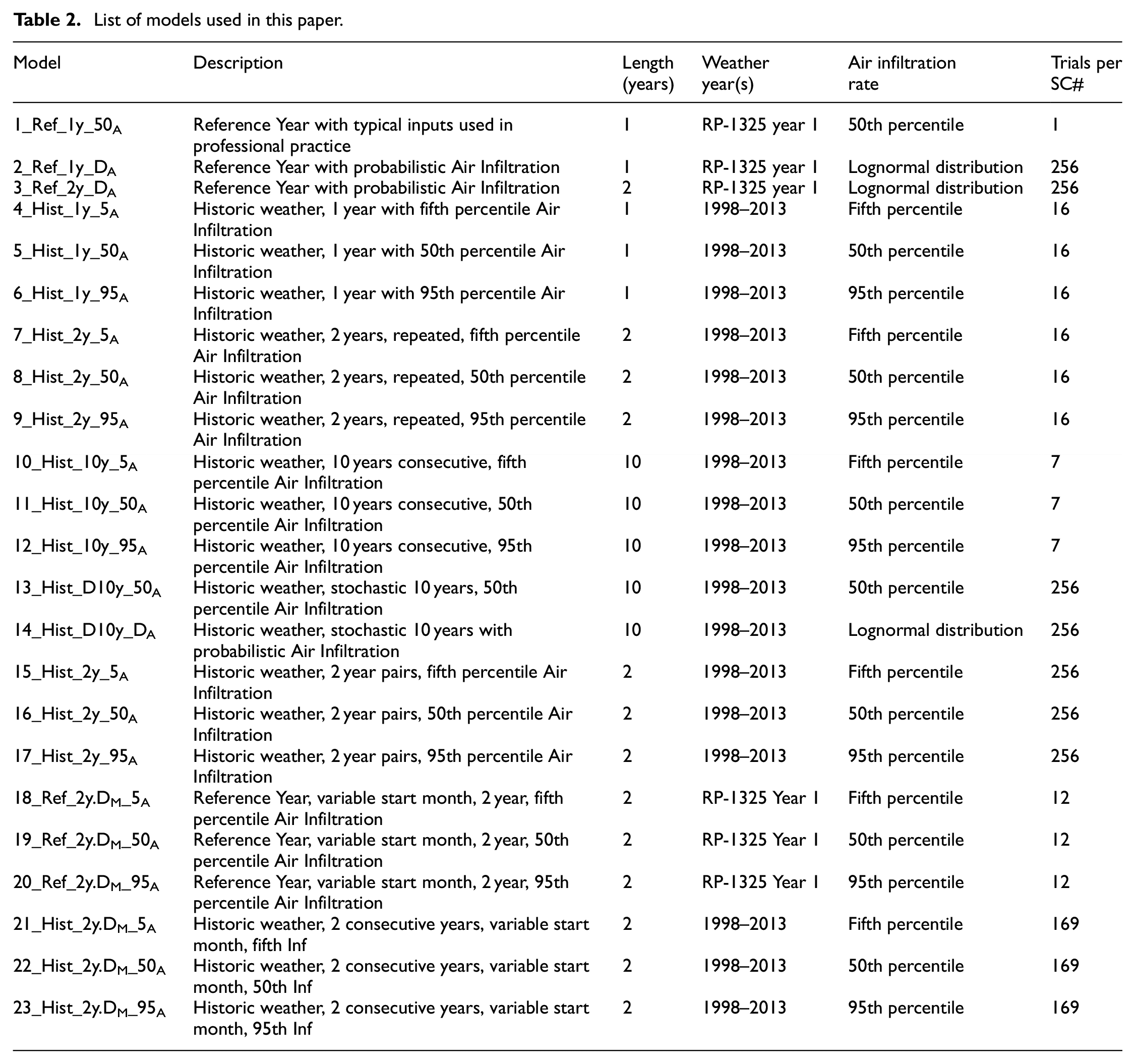
This project probabilistically sampled published lognormal distributions for air infiltration rates (El Orch et al., 2014) of buildings when simulating moisture outcomes to examine the range of moisture outcomes due to air infiltration for both reference year and historic multi-year (2- and 10-year) simulations. Table 2 shows the list of 23 simulation models used in this paper. The model names are based on #, weather year data, length of simulation, and air infiltration rate. Ref denotes the model uses a reference year. Hist denotes the model uses 1998–2013 weather year(s). D denotes a distribution (for sampling). A number followed by y denotes the length of simulation in years (e.g. 2 y denotes a 2-year simulation period). #_A denotes the air infiltration rate used (e.g. 5_A is the fifth percentile value) from the lognormal distribution. D_M denotes that the model used a distribution for the starting month of the simulation period. The “trials per SC#” value is the number of simulation trials performed for each of the four assembly scenarios (listed in Table 1).

Table 2.

List of models used in this paper.

Model	Description	Length (years)	Weather year(s)	Air infiltration rate	Trials per SC#
1_Ref_1y_50_A	Reference Year with typical inputs used in professional practice	1	RP-1325 year 1	50th percentile	1
2_Ref_1y_D_A	Reference Year with probabilistic Air Infiltration	1	RP-1325 year 1	Lognormal distribution	256
3_Ref_2y_D_A	Reference Year with probabilistic Air Infiltration	2	RP-1325 year 1	Lognormal distribution	256
4_Hist_1y_5_A	Historic weather, 1 year with fifth percentile Air Infiltration	1	1998–2013	Fifth percentile	16
5_Hist_1y_50_A	Historic weather, 1 year with 50th percentile Air Infiltration	1	1998–2013	50th percentile	16
6_Hist_1y_95_A	Historic weather, 1 year with 95th percentile Air Infiltration	1	1998–2013	95th percentile	16
7_Hist_2y_5_A	Historic weather, 2 years, repeated, fifth percentile Air Infiltration	2	1998–2013	Fifth percentile	16
8_Hist_2y_50_A	Historic weather, 2 years, repeated, 50th percentile Air Infiltration	2	1998–2013	50th percentile	16
9_Hist_2y_95_A	Historic weather, 2 years, repeated, 95th percentile Air Infiltration	2	1998–2013	95th percentile	16
10_Hist_10y_5_A	Historic weather, 10 years consecutive, fifth percentile Air Infiltration	10	1998–2013	Fifth percentile	7
11_Hist_10y_50_A	Historic weather, 10 years consecutive, 50th percentile Air Infiltration	10	1998–2013	50th percentile	7
12_Hist_10y_95_A	Historic weather, 10 years consecutive, 95th percentile Air Infiltration	10	1998–2013	95th percentile	7
13_Hist_D10y_50_A	Historic weather, stochastic 10 years, 50th percentile Air Infiltration	10	1998–2013	50th percentile	256
14_Hist_D10y_D_A	Historic weather, stochastic 10 years with probabilistic Air Infiltration	10	1998–2013	Lognormal distribution	256
15_Hist_2y_5_A	Historic weather, 2 year pairs, fifth percentile Air Infiltration	2	1998–2013	Fifth percentile	256
16_Hist_2y_50_A	Historic weather, 2 year pairs, 50th percentile Air Infiltration	2	1998–2013	50th percentile	256
17_Hist_2y_95_A	Historic weather, 2 year pairs, 95th percentile Air Infiltration	2	1998–2013	95th percentile	256
18_Ref_2y.D_M_5_A	Reference Year, variable start month, 2 year, fifth percentile Air Infiltration	2	RP-1325 Year 1	Fifth percentile	12
19_Ref_2y.D_M_50_A	Reference Year, variable start month, 2 year, 50th percentile Air Infiltration	2	RP-1325 Year 1	50th percentile	12
20_Ref_2y.D_M_95_A	Reference Year, variable start month, 2 year, 95th percentile Air Infiltration	2	RP-1325 Year 1	95th percentile	12
21_Hist_2y.D_M_5_A	Historic weather, 2 consecutive years, variable start month, fifth Inf	2	1998–2013	Fifth percentile	169
22_Hist_2y.D_M_50_A	Historic weather, 2 consecutive years, variable start month, 50th Inf	2	1998–2013	50th percentile	169
23_Hist_2y.D_M_95_A	Historic weather, 2 consecutive years, variable start month, 95th Inf	2	1998–2013	95th percentile	169

Envelope assemblies and material properties

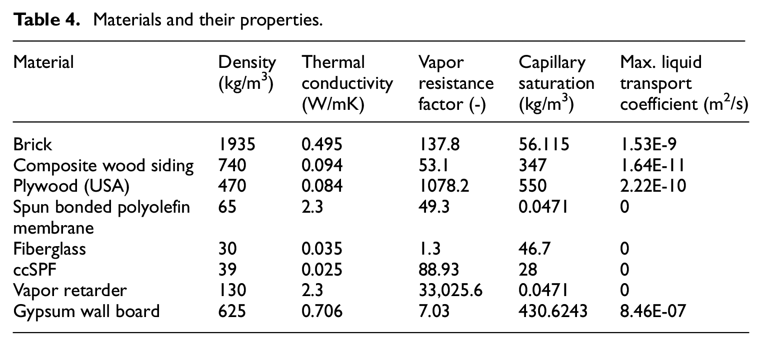
This project uses four common wood framed wall assemblies that were analyzed using weather conditions in Philadelphia, Pennsylvania, USA that have been used in previous studies (Chung et al., 2020). The four scenarios listed in Table 1 vary based on two cladding materials and two insulation types. Each wall assembly has six layers of construction. (1) An exterior cladding adjacent to an air gap, (2) a water + air barrier membrane, (3) sheathing, (4) thermal insulation within a wood framed cavity, (5) a vapor retarder, and (6) an interior finish material. The material thicknesses are listed in Table 3 and are based on common sizes used in construction that the author has experienced within professional practice. The materials’ hygrothermal properties are listed in Table 4. The material properties are either derived from ASHRAE RP-1018 Research Report: A Thermal and Moisture Transport Property Database for Common Building and Insulating Materials (Kumaran, 2002) or from material properties listed in WUFI Pro 6.1. Surface transfer coefficients are shown in Table 5.

Table 3.

List of material layer thickness for modeling scenarios.

Material	Thickness	Material	Thickness	Material	Thickness
Material	mm	Material	mm	Material	mm
Brick	92.08	Plywood	15.88	Gypsum Board	12.7
Wood siding	9.53	Insulation	139.7

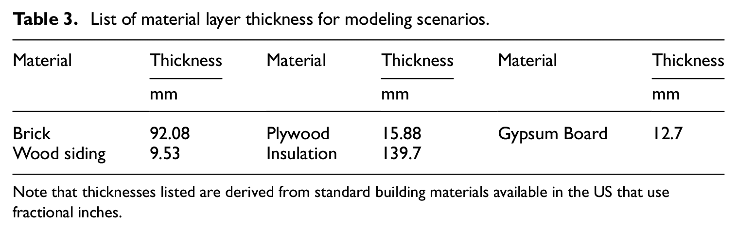
Note that thicknesses listed are derived from standard building materials available in the US that use fractional inches.

Table 4.

Materials and their properties.

Material	Density (kg/m³)	Thermal conductivity (W/mK)	Vapor resistance factor (-)	Capillary saturation (kg/m³)	Max. liquid transport coefficient (m²/s)
Brick	1935	0.495	137.8	56.115	1.53E-9
Composite wood siding	740	0.094	53.1	347	1.64E-11
Plywood (USA)	470	0.084	1078.2	550	2.22E-10
Spun bonded polyolefin membrane	65	2.3	49.3	0.0471	0
Fiberglass	30	0.035	1.3	46.7	0
ccSPF	39	0.025	88.93	28	0
Vapor retarder	130	2.3	33,025.6	0.0471	0
Gypsum wall board	625	0.706	7.03	430.6243	8.46E-07

Table 5.

Surface transfer coefficients.

Exterior surface	Heat transfer coefficient (W/m² K)	17
Exterior surface	Vapor transfer coefficient (kg/sm² Pa)	7.40E-08
Interior surface	Heat transfer coefficient (W/m² K)	8
Interior surface	Vapor transfer coefficient (kg/sm² Pa)	2.30E-08

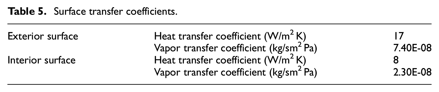
The exterior surface values are based on the default exterior wall values for a surface with “No coating” in WUFI Pro as detailed in the software and manual and is related to the Heat Resistance value used. The WUFI Pro manual topic 28 “Water Vapor Transfer Coefficients” provides the following “example, the water vapor transfer coefficients 8.0E-8 (exterior) and 2.2E-8 kg/m²sPa (interior) result from WUFI’s default heat transfer resistances 1/α of 0.056 and 0.13 m²K/W, respectively” (Zirkelbach et al., 2007). The Heat Resistance value of 0.0588 m² K/W is the provided input when selecting and “External Wall” in WUFI Pro. The reciprocal value, 17 W/(m² K) is the Heat Transfer Coefficient used in this paper for the exterior surface. WUFI Pro Help Topic 28, also states that the Water Vapor Transfer Coefficient can be determined from the convective component of the heat transfer coefficient a_c in W/m² K, by multiplying it by 7E-9. The convective component of the heat transfer coefficient is stated to be estimated as the Heat Transfer Coefficient minus 6.5 W/(m² K) for the exterior surface. Thus, a_c = 17–6.5 = 10.5 W/(m² K) and the Vapor Transfer Coefficient for the exterior surface = 7E-9 × 10.5 = 7.4E-8 kg/sm² Pa. Likewise the Heat Resistance Value for the interior surface defaults to 0.125 in WUFI Pro when selecting an exterior wall. This reciprocal value of 8 W/m² K is used as the Heat Transfer Coefficient of the interior wall surface in this paper and the resulting Vapor Transfer Coefficient is 2.2E-9 kg/sm² Pa for the air layer at the indoor surface. The US DOEBTO Guidelines recommends modeling an interior latex paint layer as 10 perms. A value of 10 perms is approximately 5.7E-10 kg/(sm² Pa). Adding the paint to the air layer gives a combined Vapor Transfer Coefficient of approximately 2.3E-8 kg/(sm² Pa). While dynamic wind-dependent exterior surface transfer coefficients can be modeled in WUFI Pro, that capability has not yet been implemented in HAM-Tools and was outside the scope of this paper.

Boundary conditions including wind-driven rain

When simulating building envelope H.A.M. transport both indoor and outdoor boundary conditions are needed. HAM-Tools can use eight input parameters for hourly outdoor weather: air temperature, dewpoint temperature (which is used with air temperature to directly calculate RH), irradiation solar global on horizontal, irradiation solar diffuse on horizontal, clear sky direct normal irradiation, long wave radiation, wind direction, wind speed, and rain accumulation.

Moisture reference year weather data originally published as part of ASHRAE RP-1325 was used in this research project. Weather data used in the historic 10-year data sets are derived from datasets available via the US National Oceanic and Atmospheric Administration (NOAA) website. At the time of the research project complete hourly weather data (including rain accumulation) suitable for deriving weather inputs in HAM-Tools was available for 16 years (1998–2013) for Philadelphia. The weather data from these 16 years were used in this project.

Wind-driven rain is a significant source of moisture at the exterior surface of the building envelope. ASHRAE Standard 160-2016 provides a numerical method for estimating rain deposition on vertical walls that accounts for wind direction with respect to wall orientation, wind speed, and rainfall intensity on a horizontal surface. For this project, walls were simulated as facing north. Researchers have stated that in the US and Canada, north facing walls predominantly experience increase moisture levels as they have less solar radiation exposure to assist in drying (Salonvaara et al., 2011). The steps to implement these moisture sources in HAM-Tools have been detailed and verified using WUFI Pro 6.1 in previous work (Chung et al., 2020).

For the indoor boundary condition HAM-Tools by default utilizes functions defined in EN15026 and ASHRAE Standard 160-2016 to determine the varying indoor air temperature and relative humidity that is based on the varying outdoor air temperature and indoor occupancy. In this project a normal occupancy and medium moisture load was used. This results in an indoor temperature range between 20°C and 25°C while the relative humidity range is between 30% and 60% depending on outdoor temperature.

Hygrothermal analysis evaluation criteria

ASHRAE Standard 160-2016 provides criteria for moisture performance evaluation of building envelopes. It provides guidance on appropriate analysis procedures and needed design parameters (inputs for the analysis) (ASHRAE, 2016). Researchers have studied mold growth rates and have used experimental measurements to develop a mathematical model for mold growth on wood (pine and spruce) building materials (Hukka and Viitanen, 1999). ASHRAE Standard 160-2016 integrates the VTT model into the evaluation criteria and states that the surfaces of building envelope assemblies shall not exceed a mold index value of three. A mold index value of three has a description of “Visual findings of mold on surface, <10% coverage, or <50% coverage of mold (microscope).” The authors of WUFI Bio also include the VTT model and suggest that a mold index value of 2 and above is “usually not acceptable” and a mold index value below 0.5 is considered “usually acceptable” (Sedlbauer et al., 2011).

Researchers have studied the corrosion rates of metal fasteners within wood products (Zelinka, 2013). This is of importance as many building envelope assemblies use metal fasteners to mechanically connect and attach components to wood sheathing and framing. The rate of corrosion has been experimentally linked to the moisture content of the wood substrate. ASHRAE Standard 160-2016 states that “Requirements for prevention of corrosion shall be derived from the properties and function of the particular metals used in construction. If no such information is available, the 30-day running average of hourly values of surface relative humidity of the metal shall remain less than 80% in order to avoid corrosion.”

Air infiltration

Air infiltration, the bulk flow of air movement through the building envelope has been modeled using the US DOEBTO guidelines for framed walls with ventilated cladding. Building envelope simulation tools such as WUFI Pro 6.1 and HAM-Tools are inherently one-dimensional models, however air flow within ventilated envelope assemblies are multi-dimensional which is covered by the US DOEBTO guidelines with workarounds by using “Air Change Sources” within air gap layers in the assembly. These air change sources represent air changes between the air gap layer and the outdoor air or from the air gap layer and the indoor air. Three air gap layers were modeled in each envelope assembly.

Air infiltration rates are known to vary depending on the air tightness of building envelope construction as well as air pressure differences between the indoor and outdoor environments. For the two air gaps included, to account for flanking flow air infiltration, the 10 ACH value was modified to incorporate stochastic sampling as detailed in the section titled “Monte Carlo and uncertainty propagation”.

Mold growth and corrosion

Mold growth was added to HAM-Tools using the VTT model (Hukka and Viitanen, 1999) which has been adopted by ASHRAE Standard 160-2016. The location of mold growth that was observed to have the highest values and be of concern was on the inside facing surface of the plywood sheathing. This would be expected to be the area of concern for mold growth as this surface is made of wood, is on the cold side of the thermal insulation, and inboard of the water + air barrier layer. Most materials inboard of the water + air barrier layer are generally consider to be less moisture tolerant and expected to be in relatively dry conditions. Mold growth on the plywood sheathing on the surface that faces the framing cavity could be a concern as air exchange between the cavity and the indoor air is expected to some degree. Corrosion risk analysis was performed using the ASHRAE Standard 160-2016 criteria by determining the number of hours that “the 30-day running average of hourly values of surface relative humidity of the metal shall remain less than 80% in order to avoid corrosion.” The location that was observed to have the highest values was on the inside facing surface of the plywood sheathing.

Weather

ASHRAE Research Project Report RP-1325 Environmental Weather Loads for Hygrothermal Analysis and Design of Buildings examined the used of moisture reference years for the United States and Canada as recommended in previous approaches (Salonvaara et al., 2011). They found that previous approaches were not well suited for North American climate zones and evaluated an alternative method to select an appropriate moisture reference year. A damage function, a second order polynomial equation using average yearly weather parameters, was found to be accurate (on average 85%, minimum 69%, maximum 94%) at selecting worst case weather years for the modeled buildings and locations. A product of the ASHRAE RP-1325 report is a set of moisture reference years determined using the damage function method for hygrothermal analysis for 100 locations in the US and seven locations in Canada. These moisture reference years are available for use in the commercial hygrothermal software WUFI Pro 6.1 (Zirkelbach et al., 2007) when evaluating building envelopes in one of the 107 North American locations published in RP-1325. The reference years used in this paper are from ASHRAE RP-1325.

In this paper the four assembly scenarios were simulated using reference years for 1- and 2-year periods. The 2-year periods used the reference year for both the first and second year. This was also done with the individual weather years (1998–2013) and pairs of historic weather years. Ten-year simulations of the historic consecutive years were also run. There are seven sets of historic 10-year data from the 16 consecutive years available in this study. The first being 1998–2007 and the last being 2004–2013. These non-stochastic trials are helpful for comparison with the stochastic models.

Damage function

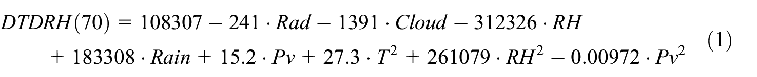
This project utilized the damage function developed in ASHRAE RP-1325 which attempts to score weather years in terms of potential moisture damage for building envelopes. The damage function is shown in equation (1) and is also known as the RHT-index(70) and is sometimes referenced as RHT(70). This is meant to approximate the annual summation of the relative humidity multiplied by the temperature when the relative humidity is at or above 70%.

D T D R H (70) = 108307 - 241 \cdot R a d - 1391 \cdot C l o u d - 312326 \cdot R H + 183308 \cdot R a i n + 15.2 \cdot P v + 27.3 \cdot T^{2} 261079 \cdot R H^{2} - 0.00972 \cdot P v^{2}

(1)

$T$ = Average yearly ambient air temperature, °C

$RH$ = Average yearly relative humidity, %

$Rad$ = Average yearly solar radiation on the wall surface, W/m²

$Cloud$ = Average yearly cloud index, (0–8)

$Rain$ = Average yearly wind driven rain on the wall, kg/(hm²)

$Pv$ = Average yearly water vapor pressure, Pa

This was used to score the ASHRAE RP-1325 weather years as well as the 16 weather years of 1998–2013 that are used in this paper.

Monte Carlo and uncertainty propagation

Monte Carlo trials were used for uncertainty propagation of 10-year weather data and air infiltration. Ten-year weather data was assembled using weather from 1998 to 2013 by concatenating randomly selected weather years. Each weather year included hourly data for the entire year. A uniform distribution was used in selecting the years. Unlike typical meteorological years (TMY) that sample average months and concatenate them into a year, in this project, whole years were concatenated to create 10-year weather datasets. For example, one of the trials used the following years and order for weather years: 2008, 2010, 2003, 2012, 2005, 2001, 1999, 2010, 2011, 2006.

Air infiltration rates were sampled from a published lognormal distribution. Researchers (El Orch et al., 2014) have modeled the statistical distribution of air exchange rates due to infiltration for homes in the U.S. building stock resulting in a geometric mean (GM) of 0.44 h⁻¹ and a geometric standard deviation (GSD) of 2.04 h⁻¹. For this distribution the fifth percentile is approximately 0.14 h⁻¹, the 50th percentile is 0.44 h⁻¹, and the 95th percentile is about 1.4 h⁻¹. The air infiltration rate sampled was used to modify the 10 ACH (see the section titled “Air infiltration”) used in the 5 mm air gap layers included to model flanking air flow through the envelope. 10 ACH is meant to represent a typical air infiltration rate as recommended by the US DOEBTO guidelines, and in this project is correlated to the 0.44 h⁻¹ geometric mean in the lognormal distribution. For instance, if the 25th percentile value is sampled from the lognormal distribution a value of 0.27 h⁻¹ is determined. The 10 ACH in the model is multiplied by the sampled value divided by the geometric mean (thus 10 ACH × 0.27 h⁻¹/0.44 h⁻¹) resulting in a 6.1 ACH used in the model for the 25th percentile value. In this way probabilistic variation for air infiltration is included in project. Note that ACH and h⁻¹ are the same units; in this paper ACH is used to denote the parameter used in the simulation model and h⁻¹ is used to denote the lognormal distribution and sampled values. The distribution for the air infiltration rate is shown in Figure 2.

Figure 2.

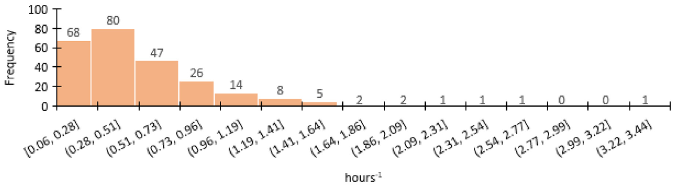
Frequency distribution of air changes per hour via air infiltration (GM = 0.44 h⁻¹ GSD = 2.04 h⁻¹) in 256 trials.

Latin Hypercube Sampling (LHS) was employed. This established the list of weather and air infiltration input parameters and created 256 probabilistic trials for each of the four envelope assemblies. When using Monte Carlo methods often thousands of trials will be used, however given the length of time and computational expense of 10-year simulations, running thousands of simulations for each scenario was not feasible. Annex 55 researchers showed that complex building simulations can be stochastically studied with as few as 100 Monte Carlo trials when using LHS and space filling methods (Hagentoft et al., 2015).

Regression analysis

The climate input parameters (T, RH, Rad, Cloud, Rain, and Pv) used in the RP-1325 damage function (see the section titled “Damage function”) were chosen as predictors for the regression analysis. (Note that Rain = Average yearly wind driven rain on the wall, kg/(hm²).) Squared values of each of the parameters were also used as predictors. For models (18–23) that used a variable starting month of a 2-year simulation period, the annual averages for the input parameters were based on 365-day periods beginning in the start month of the simulation. The responses used in the regression analysis are maximum moisture content in the plywood sheathing layer, maximum mold index value on the plywood sheathing, and hours exceeding the ASHRAE Standard 160-2016 corrosion criterion of the plywood sheathing. As the mold and corrosion analysis are surface specific, the indoor facing (warm side in winter) surface of the plywood was used for the evaluations.

Results and discussion

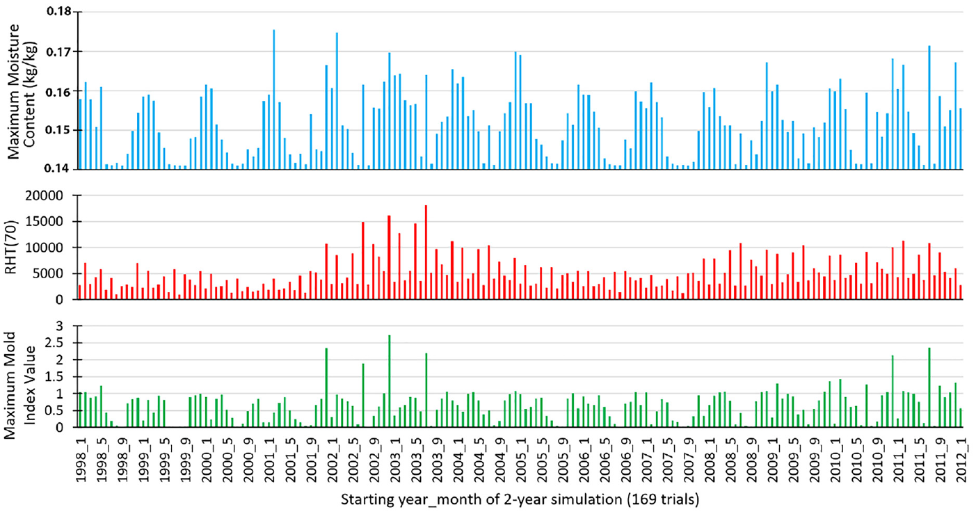
Damage function values (using equation (1)) for the ASHRAE RP-1325 reference years and the 16 historic years (1998–2013) for Philadelphia are shown in Figure 3. The single year damage function value, RHT-index(70), is shown by the blue bars. The orange striped bars show the highest damage function value for 365 consecutive days that exists within a consecutive 2-year period. This is of interest because it indicates that the selection of moisture reference year may also benefit from exploring variable starting points. For instance, the weather years 1999 and 2000 each have relatively low annual damage function values when evaluated from January through December, however a much larger value exists for the 365-day period starting in mid-August of 1999 and ending in mid-August of 2000.

Figure 3.

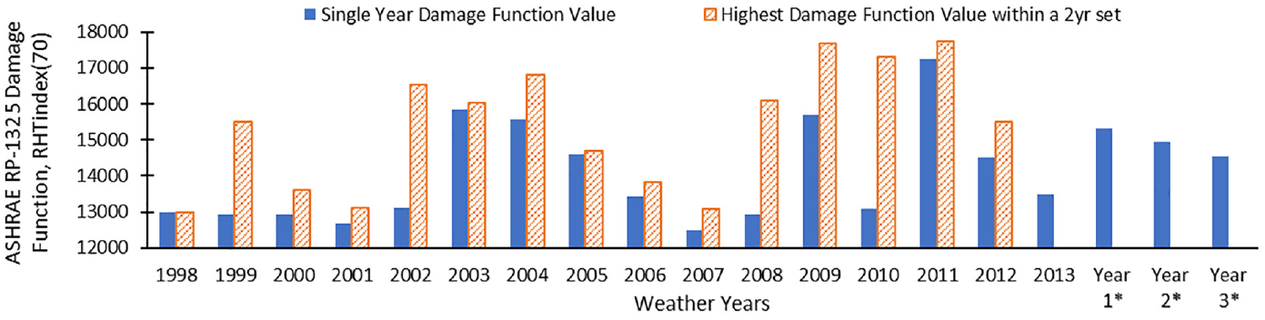
Damage function values for Philadelphia Weather years 1998–2013 with ASHRAE RP-1325 reference years denoted with an asterisk.

ASHRAE RP-1325 used weather data from 1961 to 1990. The actual year numbers for Years 1, 2, and 3 that are included in WUFI Pro are not known, however given the dates used in RP-1325 it is not surprising that the damage function values are not identical to any of the 16 more recent years used in this paper. There are 4 years (2003, 2004, 2009, and 2011) that have annual damage function values (January through December) greater than the value for Year 1. RP-1325 intended that the Year 1 moisture reference year would represent the 10th percentile worst moisture year for the 1961–1990 weather years. In this paper the Year 1 damage function value is near the 25th–30th percentile highest January through December annual damage function value. Given the values seen in Figure 3 it is reasonable to predict that there may be years that yield greater moisture related damage in the simulations than if simulated with the Year 1 weather.

Baseline results

All four scenarios (assemblies listed in Table 1) were simulated using the ASHRAE RP-1325 “year 1” moisture-design reference year for Philadelphia, that is packaged with WUFI Pro. The air exchange rates are modeled using the recommendations listed in the US DOEBTO guidelines for ventilate cladding. These simulations (Model 1_Ref_1yr_50_A) using the reference years are referred to in this paper as the baseline and are meant to represent assessments made in standard practice without probabilistic methods. Time series graphs of the moisture content in the sheathing for each of the scenarios using both HAM-Tools and WUFI Pro were previously reported (Chung et al., 2020). Mold growth and corrosion analysis were also determined for the four baseline scenarios. Table 6 summarizes three simulation degradation outcomes that had significant values and were evaluated in all 23 models for each assembly scenario.

Table 6.

Summary of baseline outcomes for all four scenarios when using ASHRAE RP-1325 reference year. Right side denotes the surface faces toward the inside.

Analysis outcomes	RP-1325 year 1 single year results
Analysis outcomes	SC1	SC2	SC3	SC4
Hours when the 30-day running average of relative humidity at the right surface of the plywood sheathing exceeds 80%	339	385	672	832
Maximum mold index value at the right surface of the sheathing	0.8	0.2	0.9	0.4
Maximum moisture content of the plywood sheathing (kg/kg)	0.154	0.141	0.157	0.156

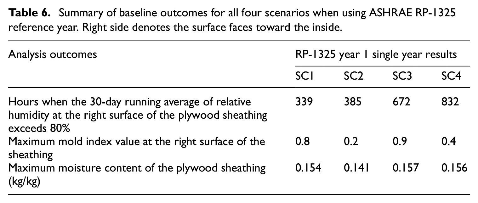
In the baseline results the maximum moisture content ranges from approximately 0.14 to 0.16 kg/kg. The moisture storage function for the plywood sheathing is shown in Figure 4. Comparing the maximum moisture content from the simulation outcomes with the moisture storage function, the moisture content corresponds to relative humidities near or greater than 80%. This is somewhat expected as the starting relative humidity for all materials in the assembly are set to 80%. While those values are on the higher end, the growth of mold is also dependent on relative humidity, temperature, and duration (wetting and drying). From Table 6 it can be seen that two of the four scenarios had greater than 650 h when the 30-day running average of the relative humidity at the right surface of the plywood sheathing exceeds 80%. However, the maximum mold index values at the plywood sheathing were all less than 1. Thus, the assumption from the baseline simulations is that mold growth on the plywood is not a significant issue. Corrosion analysis shows that although the 30-day running average of the relative humidity at the face of the plywood does have hundreds of hours of occurrence in Scenarios 3 and 4, the predicted accumulated corrosion over the 1 year period for metal embedded in the sheathing is very low at 0.006 and 0.007 µm respectively when using a prediction model develop by the USDA Forest Product Laboratory (Zelinka et al., 2011). For a typical 16D nail with a shank diameter of 4.191 mm this would be a loss of less than 0.001% of the cross-sectional area. Thus, for the studied scenarios under the baseline conditions (Model 1), the simulation results do not indicate any significant moisture related performance problems.

Figure 4.

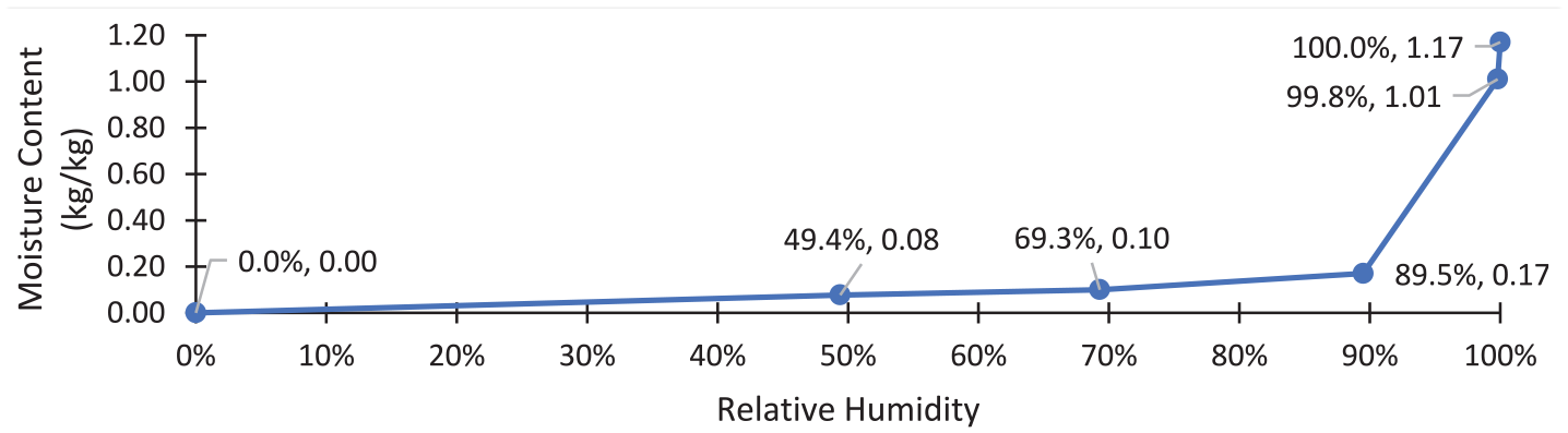
Moisture storage function for plywood sheathing, from material data listed in WUFI Pro 6 for Plywood (USA).

Reference year compared to more recent historic years (1998–2013)

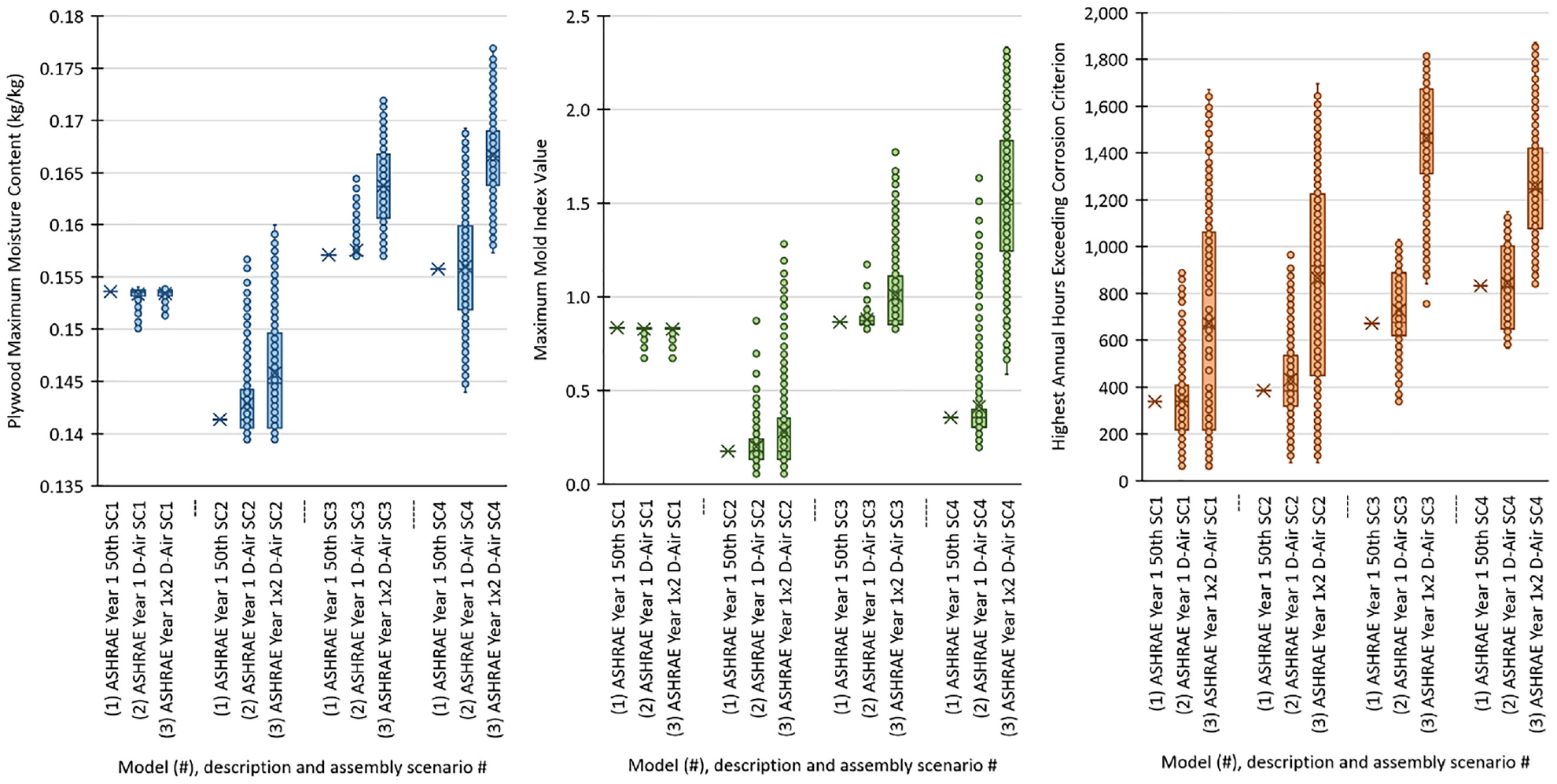
For each of the four scenarios the reference year (RP-1325 Year 1) results were compared to results from simulations using more recent historic weather years (1998–2013). Each assembly scenario (SC1–4) was modeled in an identical manner as the reference year except for the weather year input. The more recent historic years were simulated over 1 year, 2 years (by repeating 1 year and different year pairs), 10 consecutive years (e.g. 1998–2007), and 10 randomly selected years. Figure 5 shows the results when all of the models use the same steady state air infiltration rate as recommended by the US DOEBTO. In this paper this infiltration rate is referred to as the 50th percentile air infiltration rate and meant to represent what is used in typical simulations done by building envelope professionals.

Figure 5.

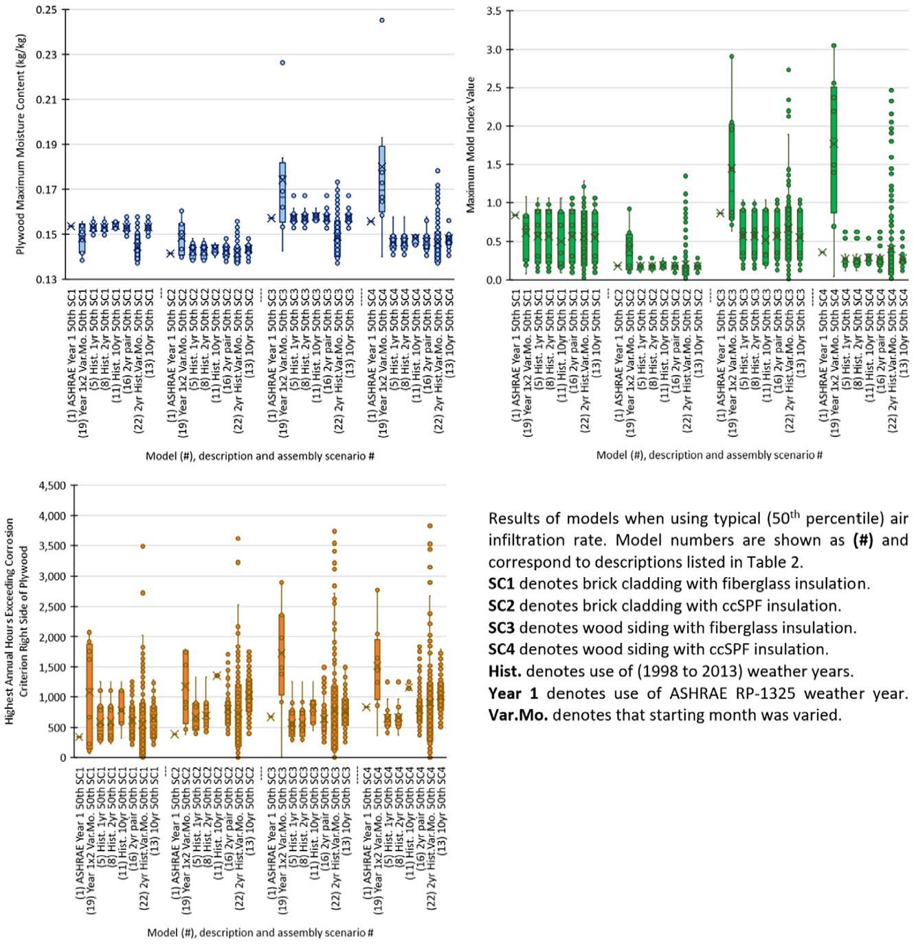
Box and whisker plots for models using reference year and more recent historic years. Left top (blue) shows distribution of plywood maximum moisture content. Right top (green) shows distribution of plywood mold index values. Left bottom (orange) shows distribution of highest annual hours exceeding ASHRAE Standard 160-2016 corrosion criterion.

In the upper left portion of Figure 5 one can see the maximum moisture content in the plywood sheathing layer predicted in the simulations, and that the baseline (Model 1) values are generally within the middle of the range (between the 25th and 75th percentile) of results for the various models using more recent historic weather years, except for Scenario 4. For Scenarios 1 and 3 (SC1 and SC3) which use fiberglass insulation the baseline results align very closely to the median values for the models using more recent historic weather years. For Scenario 2 (SC2) the baseline result is slightly lower than the median values for the historic model results. For Scenario 4 (SC4) the reference year result is at the upper end of the results for models using more recent historic weather years. Overall, the baseline model’s maximum moisture content results appear to align well with the results from models using more recent historic weather years. Models 19 and 22 used variable starting months for 2-year simulation periods. For these two models the range of moisture content results are significantly wider than the other models in all assembly scenarios and show the importance of considering the starting month of the simulation period on the results.

In the upper right portion of Figure 5 one can see the maximum mold index values that occurred on the indoor facing surface of the plywood sheathing predicted in the simulations. The results from models using more recent weather years generally have mold index median values that are lower than the baseline (Model 1) values, except in the case of Model 22 which uses a variable starting month. The baseline (Model 1) mold index values are generally near the upper end of the historic models’ mold index values for assembly Scenarios 1, 3, and 4 when using simulation periods starting in January. Scenarios 2, 3, and 4 show the mold index value of the baseline result are in the lower end of the range of results when compared with the Model 19 and 22 results.

In the lower portion of Figure 5 the worst annual hours exceeding the ASHRAE Standard 160-2016 corrosion criterion is compared across the reference year and models using more recent historic years. As some of the historic models are 2- or 10-year models the results are for the worst consecutive 365-day totals for the hours not meeting the corrosion criterion. This way the baseline and multi-year models can be shown on the same scale. The plywood sheathing has a significant range of results in the models using more recent historic years and many models have values where the median is above the baseline results. What is interesting overall for Figure 5 is that the 1-, 2-, and 10-year models using more recent historic years have very similar result ranges when the simulation period starts in January. In addition, the baseline (Model 1) results appear to be fair risk estimators compared to the models using more recent historic years for maximum moisture content and maximum mold index value if the simulation period starts in January. For corrosion criterion however the baseline results may underpredict risk. Like previous observations, the range of results for Models 19 and 22 for corrosion criterion analysis are much greater than the other models within the same assembly scenario and show that varying starting month has significant impact on the predict results.

Probabilistic air infiltration model results

For each of the four scenarios the reference year (RP-1325 Year 1) was also simulated using a probabilistic air infiltration rate over 1- and 2-year (repeating the reference year) simulation periods. Two hundred fifty-six trials were performed for each combination of assembly scenario and simulation length. Each assembly scenario (SC1–SC4) was modeled in an identical manner as the reference year except for the air infiltration rate which was sampled from a lognormal distribution (0.44 h⁻¹ GM 2.04 h⁻¹ GSD) with the geometric mean correlated to the US DOEBTO guidelines recommended air infiltration rate.

Figure 6 shows the maximum moisture content in the plywood sheathing, the maximum mold index values, and the hours not meeting the ASHRAE Standard 160-2016 corrosion criterion for the plywood for the reference year model with and without probabilistic air infiltration. Models 1, 2, and 3 use a simulation period starting with January. For Scenario 1 the baseline model using the standard non-probabilistic air infiltration rate aligns well with the maximum values from the probabilistic results for maximum moisture content and mold index values. For the remaining scenario assemblies (SC2, SC3, SC4) and for the corrosion criterion for SC1 the reference year non-probabilistic result appears to be at the lower end of the distribution of values. In particular, the 2-year probabilistic air infiltration models indicate the potential for significantly higher moisture content, mold, and corrosion than the non-probabilistic model. Given that the air infiltration is modeled as both an air source and moisture source it is not entirely surprising to see that probabilistic infiltration would have a significant impact on the distribution of results. There is added significance to this since often a buildings’ air tightness can change over time as they age due to the deterioration of sealants, adhesives, as well as movement due to material thermal expansion and contraction.

Figure 6.

Box and whisker plots for models using reference years with and without probabilistic air infiltration. Left (blue) shows distribution of plywood maximum moisture content. Middle (green) shows distribution of plywood mold index values. Right (orange) shows distribution of highest annual hours exceeding ASHRAE Standard 160-2016 corrosion criterion.

Figure 7 shows the results for Scenario 2 (brick cladding with ccSPF insulation) using the reference year for a 2-year simulation with a probabilistic distribution of air infiltration rates (Model 3, 256 trials). It is clear that the maximum moisture content, maximum mold index, and corrosion related values increase as the air infiltration rate increases when coupled with the reference year for the studied assembly scenario.

Figure 7.

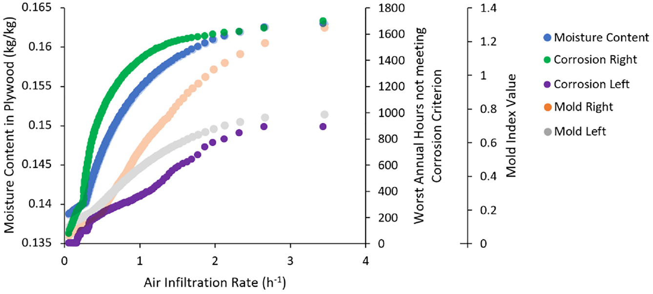
Plot for Model 3, Scenario 2, 256 trials: maximum moisture content, maximum mold index value, and highest annual hours not meeting ASHRAE Standard 160-2016 corrosion criterion versus air infiltration rate. Left denotes left side of plywood facing toward outdoors, Right denotes right side of plywood facing toward indoors.

More recent historic years (1998–2013) coupled with probabilistic air infiltration model results

For each of the four assembly scenarios probabilistic combinations of air infiltration and more recent historic years were simulated. Each assembly scenario (SC1–4) was modeled in an identical manner as the reference year except for the weather year input and air infiltration rate. The models using more recent historic years were simulated over 1 year, 2 years (by repeating 1 year), 10 consecutive years (e.g. 1998–2007), and 10 randomly selected years. For the 1-, 2-, and 10-consecutive year models, 5th, 50th, and 95th percentile air infiltration rates were used (Models 4–12 in Table 2). This was done to see if they would produce similar ranges with less computational expense to the larger 256 trials done per scenario in model 14 (10-year historic weather randomly sampled with probabilistic air infiltration).

Figure 8 shows the range of results for Scenarios 1 and 2 for each of the historic weather years (1998–2013) for moisture content, mold index value, and annual hours exceeding the corrosion criterion when using 5th, 50th, and 95th percentile probabilistic air infiltration rates (models 4, 5, and 6). These simulations start with January and are 1 year in length. One would expect from the reference year probabilistic air infiltration rate model results (seen in Figure 7) that increased air infiltration would consistently lead to higher moisture content, mold index, and corrosion related results. However, from the Model 4, 5, and 6 results seen in Figure 8, the results show that in some cases the 5th or 50th percentile air infiltration rate will result in higher moisture, mold, and/or corrosion related values than when using the 95th percentile air infiltration rate. Figure 8 also shows that the predicted ASHRAE RP-1325 Damage Function values may not have a close relationship with expected moisture, mold, or corrosion results. For instance, for Scenario 1, the 2011 weather year has the highest Damage Function value but results in the fourth highest moisture content in the plywood sheathing. This is more pronounced in the mold index values for Scenario 1, where the 2011 weather year has one of the lowest mold index values for the right side (surface facing toward the inside) of the plywood.

Figure 8.

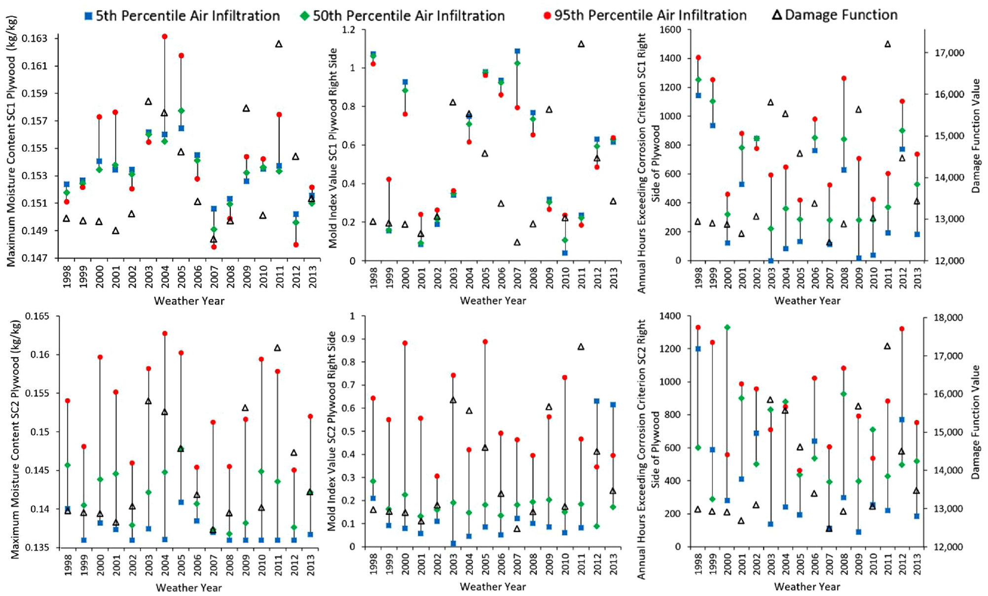
Scenario 1 (above) and Scenario 2 (below) for Models 4, 5, and 6.

Figure 9 shows the results for moisture content, mold index value, and corrosion criterion for the more recent historic year models coupled with probabilistic air infiltration rates. They also include the previous results for ease of comparison. Figure 9 shows that when using a simulation period starting in January, the coupling of probabilistic air infiltration rates with the more recent historic years (Models 4–12 and 14–17) produces a large range of moisture content values with many values that are significantly above the range produced when using probabilistic air infiltration rates with the reference year weather. However, for three of the assembly scenarios (SC2–4), the 2-year reference year simulation (starting in January) with probabilistic air infiltration produced a range that overlaps with a large portion of the more recent historic year results that also used simulation periods starting in January. In the case of the 10-year randomly selected weather years (starting in January) coupled with probabilistic air infiltration, the range of moisture content outcomes expands and shows higher upper range values. Interestingly, the probabilistic models that used the 5th and 95th percentiles (Models 4, 6, 7, 9, 10, and 12) air infiltration rates produced fairly large overlap with Model 14 (10-year models using randomly selected weather years and probabilistic air infiltration) with far less computational expense. Models 18–23 couple 2-year simulation periods with variable starting months with 5th, 50th, and 95th percentile air infiltration rates and the results from these models show the greatest range of moisture content, mold, and corrosion analysis results out of all of the models studied. The range is significantly more than those from the Model 3 results. Recall that Model 3 uses a 2-year simulation period starting in January using the ASHRAE RP-1325 Year 1 reference year coupled with a probabilistic distribution of air infiltration rates (256 trials). This again suggests that using a variable starting month may be an important consideration when attempting to select a simulation period. Figure 10 shows the maximum moisture content, RHT-index, and mold index values that occurred in 169 trials of Model 22 for Scenario 3 using varying starting months. There do appear to be some cyclical patterns in the mold index results with lower values consistently occurring with simulations that started in July, September, and October, however this observation is likely only valid for the location studied (Philadelphia) and would most likely produce different patterns for other locations.

Figure 9.

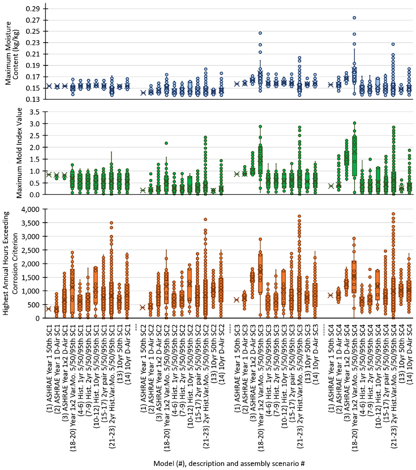
Box and whisker plots for all 23 models studied. Upper (blue) portion shows maximum moisture content in the plywood. Middle (green) portion shows maximum mold index values. Lower (orange) portion shows highest annual hours exceeding ASHRAE Standard 160-2016 corrosion criterion.

Figure 10.

Scenario 3, Models 22, varying start month, maximum moisture content, RHT-index, and maximum mold per trial.

Regression analysis

After running Models 10–14 that used 10-year simulation periods, the project examined the relationship between damage function values and maximum moisture content in the plywood to see if there was a way to predict which 10-year simulation period would yield the most moisture, mold, and/or corrosion. Annual climate input parameters and annual damage functions used as predictors did not yield useable regression models to predict which 10-year weather combinations would result in the highest simulated moisture, mold, or corrosion. For instance, Figure 11 shows the distribution of maximum moisture content for Scenario 4 using Model 14 (10-year simulation period, starting in January, coupled with probabilistic air infiltration). Generally, as the air infiltration rate is increased the maximum moisture content increases, however there is a significant range of variation due to the variability of the weather years. Figure 11 also includes the moisture content as it varies with the worst year ASHRAE RP-1325 Damage Function value out of the 10 weather years in each of the 256 trials. One can see that the worst year Damage Function value by itself is not a good predictor of the moisture content in the 10-year simulations, but the range of moisture content trial outcomes does appear to expand to higher possible values as the Damage Function value increases.

Figure 11.

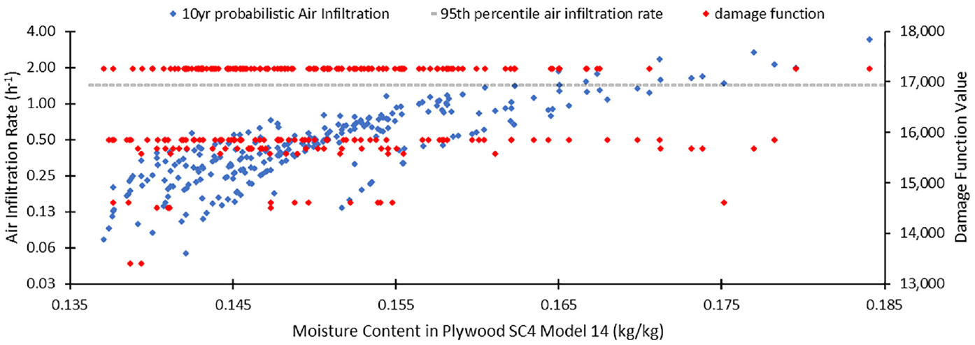
Scenario 4 Model 14 (10-year randomly selected historic weather coupled with probabilistic air infiltration rate). Maximum moisture content in plywood sheathing, 256 trials. Horizontal gray line denotes 95th percentile air infiltration rates.

Given low R² results from the regression analysis of the 10-year models, the time series data of the highest moisture content and mold growth trials were examined and generally showed that the values peaked in the first 2 years for many scenarios and models. This led to a re-examination of the 1-year and 2-year models and their time series output. For instance, in Figure 9, the 1- and 2-year models using more recent historic years with simulation periods starting with January (models 4–9) had nearly identical results. On closer inspection of the time series results it appears that the maximum moisture content frequently occurred in these models near the beginning of the simulation period as the starting relative humidity for the assembly is set to 80%. Using a starting relative humidity of the assembly at 80% is a criterion required by ASHRAE Standard 160-2016 for all non-concrete based materials and helps to simulate recently closed in sets of materials used in the envelope assembly that may occur during construction. Figure 12 shows the time series moisture content for Scenario 2 (left two graphs, brick cladding + ccSPF) and Scenario 4 (right two graphs, wood siding + ccSPF) in the plywood for the reference year above (model 3) and the 2005 weather year below (models 7, 8, and 9) when simulated over a 2-year period. The plots show the results when using the 5th, 50th, and 95th percentile probabilistic air infiltration rates. The 2005 weather year was selected for this comparison as it produced the highest amount of moisture content in the plywood for Scenario 4 out of the more recent historic weather years. From the time series plots one can see that the reference year used in Model 3 produced moisture content at the 1-year mark that was higher in all trials for Scenario 4 than at the start of the simulation. The 2005 weather year produced moisture content at the 1-year mark that was slightly above or well below the starting moisture content in Scenarios 2 and 4. This helps explain the noticeable increase in values in the 2-year reference year results compared to the 1-year reference results, as well as the more recent historic year results for Scenarios 3 and 4 which use wood siding as the exterior cladding (in contrast to Scenarios 1 and 2 which use brick cladding).

Figure 12.

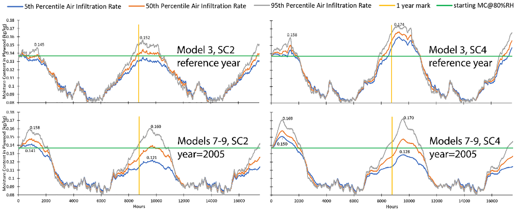
Scenario 2 (brick cladding with ccSPF insulation) on left, moisture content results and Scenario 4 (wood cladding with ccSPF insulation) on right, reference year (top) versus 2005 weather year (bottom).

The above observations led to the creation of Models 18–23 that use variable starting months with 2-year simulation periods. Regression analysis was performed for each Scenario for Model 22 (50th percentile ACH) and again the resulting models had low R² values when using annual climate predictors. In some cases the regression analysis was able to produce models for maximum moisture content between 0.7 and 0.8 however the same predictors resulted in drastically lower R² values when trying to model maximum mold index values. Looking at the maximum mold index values, the RHT-index and the maximum moisture content values for the 169 trails of Model 22 Scenario 3 in Figure 10 one can see that the highest values of moisture content do not coincide with the highest mold index values. The RHT-index used in Figure 10 is the actual simulation results observed using the plywood relative humidity and temperature values. This was done because the ASHRAE RP-1325 damage function (which is an estimated RHT-index value) did not correlate well with the results in this paper. Either way, one can see from Figure 10 that the three metrics (moisture content, RHT-index, and mold index) indicate different worst-case years and perhaps the task of trying to determine the worst-case year needs to be framed within the context of what defines the worst case.

Estimated mold index

Of the metrics used in this study mold growth is generally of highest concern to the public. If the worst-case year is defined by the one producing the highest mold growth and if the sheathing is located on the cold side of the insulation the temperatures and relative humidities of the outdoor air may be close enough to approximate the conditions at the sheathing for mold growth analysis. Thus, as a next step a maximum mold index value was estimated using the outdoor air temperature and a time-averaged outdoor relative humidity as inputs to the mold index model (equation (1)). Figure 13 shows normalized maximum mold index values that were observed in the trials for Scenarios 3 and 4 (Model 22) and compares them to the normalized values estimated when using outdoor temperature and relative humidity. As the observed relative humidity varied greatly from one time step to the next for the outdoor conditions in comparison to those at the sheathing layer (where the mold value is of interest), a time averaged value was used. Through trial and error an average of 14- and 28-days was found to produce reasonable results. From Figure 13 one can see that the estimated mold index lacks the monthly resolution that the actual trials have, however the estimate does appear to align well with the trend of higher values that occur within each year. Given the low mold index values in Scenarios 1 and 2 (nearly all the values were below 1), the correlation with the estimated mold index values were low. Scenarios 3 and 4 had greater variation and both had trial outcomes where the highest maximum mold index values were near 3. While this preliminary mold index method did not yield a useable regression model, the visual plot suggests that some version of a mold estimate may be worth further study if maximum mold growth is the assessment of interest.

Figure 13.

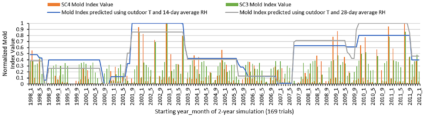
Normalized maximum mold index values for Scenarios 3 and 4, Model 22, compared to estimated mold index values using outdoor temperature and relative humidity.

Summary

This paper hypothesized that envelope hygrothermal simulations using single-year, single trial moisture reference years for weather may underestimate moisture content and related moisture damage when compared to simulations using stochastic multi-year (2- and 10-year weather data) and probabilistic air infiltration rates. In three of the four assembly scenarios (SC2–4) studied in this paper the hypothesis appears to be true. Generally, as air infiltration rates increased maximum moisture content, maximum mold index values, and corrosion results increased. Stochastic 2-year simulations appear to be as robust as stochastic 10-year simulations, as they produce very similar ranges of outcomes. Given that stochastic 10-year simulations are more computationally expensive, running stochastic 2-year simulations may be more efficient without underestimating moisture risks. There were two outcomes in the project that were not expected. First, there were cases in the trials were lower air infiltration rates yield higher moisture, mold, and corrosion results. This may be due to a reduced ability to dry out the assembly when there are low air infiltration rates and a lot of moisture has accumulated from rain penetration. This finding needs further exploration and study. Second, the simulation results were highly sensitive to the starting month of the simulation period and that the starting month with the worst moisture results can vary depending on the weather year used. This is most likely due to the starting relative humidity of the materials being set to 80% (defined by ASHRAE Standard 160) having a strong influence on the first few months of results. Two recommendations can be made from this study: (1) Variable starting months should be used in hygrothermal envelope assessments and the simulation period should be a minimum of 2-years. (2) Variable air infiltration rates (5th, 50th, and 95th) should be used in hygrothermal envelope assessment as they may have unexpected results where a tighter envelope may yield more moisture accumulation.

Footnotes

Declaration of conflicting interests

The author(s) declared no potential conflicts of interest with respect to the research, authorship, and/or publication of this article.

Funding

The author(s) received no financial support for the research, authorship, and/or publication of this article.

ORCID iD

Daniel Chung

References

ASHRAE (2016) Standard 160-2016: Criteria for Moisture Control Design Analysis in Buildings. Atlanta, GA: American Society of Heating, Refrigerating and Air-Conditioning Engineers.

Bradtmueller

Foley

(2014) Historical trends of exterior wall materials used in US residential construction. In: 50th ASC annual international conference proceedings.

Brambilla

Sangiorgio

(2020) Mould growth in energy efficient buildings: Causes, health implications and strategies to mitigate the risk. Renewable and Sustainable Energy Reviews 132: 110093.

Chitte

Sonawane

(2018) Study on causes and prevention of cracks in building. International Journal for Research in Applied Science and Engineering Technology 6: 453–461.

Chung

Wen

(2020) Development and verification of the open source platform, HAM-Tools, for hygrothermal performance simulation of buildings using a stochastic approach. Building Simulation 13: 497–514.

di Giuseppe

D’Orazio

Favi

, et al. (2017) Robust internal thermal insulation of historic buildings: Report and tool: Probability based Life Cycle Impact Assessment.

DOE (2015) Quadrennial technology review: An assessment of energy technologies and research opportunities.

El Orch

Stephens

Waring

(2014) Predictions and determinants of size-resolved particle infiltration factors in single-family homes in the US. Building and Environment 74: 106–118.

EN 15026 (2007) Hygrothermal Performance of Building Components and Building Elements – Assessment of Moisture Transfer by Numerical Simulation. Geneva: International Organization for Standardization.

10.

González-Torres

Pérez-Lombard

Coronel

, et al. (2022) A review on buildings energy information: Trends, end-uses, fuels and drivers. Energy Reports 8: 626–637.

11.

Gradeci

Berardi

(2019) Application of probabilistic approaches to the performance evaluation of building envelopes to withstand mould growth. Journal of Building Physics 43: 187–207.

12.

Hagentoft

C-E

Ramos

Grunewald

(2015) Annex 55, Reliability of Energy Efficient Building Retrofitting-Probability Assessment of Performance and Cost (RAP-RETRO): Stochastic data. Report, Chalmers University of Technology, Göteborg.

13.

Hukka

Viitanen

(1999) A mathematical model of mould growth on wooden material. Wood Science and Technology 33: 475–485.

14.

Janssen

(2013) Monte-Carlo based uncertainty analysis: Sampling efficiency and sampling convergence. Reliability Engineering & System Safety 109: 123–132.

15.

Jellen

Memari

(2019) Structural design of a typical American wood-framed single-family home. In: Concu

(ed.) Timber Buildings and Sustainability. Rijeka, Croatia: IntechOpen, pp.27–54.

16.

Kumaran

(2002) A thermal and moisture transport property database for common building and insulating materials: 1018-RP: Final report for American Society of Heating, Refrigerating and Air-conditioning Engineers. National Research Council Canada, Ottawa, ON.

17.

Lstiburek

Ueno

Musunuru

(2016) Strategy Guideline: Modeling Enclosure Design in Above-Grade Walls. Westford, MA: Building Science Corporation.

18.

Mudarri

Fisk

(2007) Public health and economic impact of dampness and mold. Indoor Air 17: 226–235.

19.

Persily

Musser

Emmerich

(2010) Modeled infiltration rate distributions for U.S. housing. Indoor Air 20: 473–485.

20.

Prada

Cappelletti

Baggio

, et al. (2014) On the effect of material uncertainties in envelope heat transfer simulations. Energy and Buildings 71: 53–60.

21.

Sadovský

Koronthályová

Matiašovský

, et al. (2014) Probabilistic modelling of mould growth in buildings. Journal of Building Physics 37: 348–366.

22.

Salonvaara

Zhang

Pezoulas

, et al. (2011) Final report: Environmental weather loads for hygrothermal analysis design of buildings. ASHRAE RP-1325. Syracuse, NY: Syracuse University.

23.

Sedlbauer

Krus

Zilig

(2011) WUFI-BIO 3 assessing the risk of mould growth. Fraunhofer Institute for Building Physics.

24.

Thomas

Marino

Muñoz

(2022) Multivariate analysis for assessing the thermal performance of vertical opaque envelopes in extended regions. Journal of Building Physics 46: 259–291.

25.

Tian

(2013) A review of sensitivity analysis methods in building energy analysis. Renewable and Sustainable Energy Reviews 20: 411–419.

26.

Tian

Heo

de Wilde

, et al. (2018) A review of uncertainty analysis in building energy assessment. Renewable and Sustainable Energy Reviews 93: 285–301.

27.

U.S. Bureau of Economic Analysis (2019) Gross domestic product by industry: Fourth quarter and annual 2018. News Release.

28.

Vereecken

Van Gelder

Janssen

, et al. (2015) Interior insulation for wall retrofitting – A probabilistic analysis of energy savings and hygrothermal risks. Energy and Buildings 89: 231–244.

29.

Wang

Defo

Xiao

, et al. (2021) Stochastic simulation of mould growth performance of wood-frame building envelopes under climate change: Risk assessment and error estimation. Buildings 11: 333.

30.

Wang

(2018) Stochastic modelling of hygrothermal performance of highly insulated wood framed walls. Building and Environment 146: 12–28.

31.

Zabel

Morrell

(2012) Wood Microbiology: Decay and Its Prevention. London: Academic Press.

32.

Zelinka

(2013) Corrosion of embedded metals in wood: An overview of recent research with implications for building moisture design. ASHRAE Transactions 119: 442–449.

33.

Zelinka

Derome

Glass

(2011) Combining hygrothermal and corrosion models to predict corrosion of metal fasteners embedded in wood. Building and Environment 46: 2060–2068.

34.

Zirkelbach

Schmidt

Kehrer

, et al. (2007). Wufi^® pro–manual. Fraunhofer Institute.

Examining the impact of stochastic multi-year weather and air infiltration on hygrothermal moisture risks

Abstract

Keywords

Introduction

Building envelope economic context

Stochastic methods, uncertainty, and sensitivity analysis of building envelopes

Limitations of existing methods

Research objective

Methodology

Envelope assemblies and material properties

Boundary conditions including wind-driven rain

Hygrothermal analysis evaluation criteria

Air infiltration

Mold growth and corrosion

Weather

Damage function

Monte Carlo and uncertainty propagation

Regression analysis

Results and discussion

Baseline results

Reference year compared to more recent historic years (1998–2013)

Probabilistic air infiltration model results

More recent historic years (1998–2013) coupled with probabilistic air infiltration model results

Regression analysis

Estimated mold index

Summary

Footnotes

Declaration of conflicting interests

Funding

ORCID iD

References