Improving efficiency in the stepped-wedge trial design via Bayesian modeling with an informative prior for the time effects

Abstract

Background

In a cross-sectional stepped-wedge cluster randomized trial comparing usual care to a new intervention, treatment allocation and time are correlated by design because participants enrolled early in the trial predominantly receive usual care while those enrolled late in the trial predominantly receive the new intervention. Current guidelines recommend adjustment for time effects when analyzing stepped-wedge cluster randomized trials to remove the confounding bias induced by this correlation. However, adjustment for time effects impacts study power. Within the Frequentist framework, adopting a sample size calculation that includes time effects would ensure the trial having adequate power regardless of the magnitude of the effect of time on the outcome. But if in fact time effects were negligible, this would overestimate the required sample size and could lead to the trial being deemed infeasible due to cost or unavailability of the required numbers of clusters or participants. In this study, we explore the use of prior information on time effects to potentially reduce the required sample size of the trial.

Methods

We applied a Bayesian approach to incorporate the prior information on the time effects into cluster-level statistical models (for continuous, binary, or count outcomes) for the stepped-wedge cluster randomized trial. We conducted simulations to illustrate how the bias in the intervention effect estimate and the trial power vary as a function of the prior precision and the mis-specification of the prior means of the time effects in an example scenario.

Results

When a nearly flat prior for the time effects was used, the power or sample size calculated using the Bayesian approach matched the result obtained using the Frequentist approach with time effects included. When a highly precise prior for the time effects (with accurately specified prior means) was used, the Bayesian result matched the Frequentist result obtained with time effects excluded. When the prior means of the time effects were nearly correctly specified, including this information improved the efficiency of the trial with little bias introduced into the intervention effect estimate. When the prior means of the time effects were greatly mis-specified and a precise prior was used, this bias was substantial.

Conclusion

Including prior information on time effects using a Bayesian approach may substantially reduce the required sample size. When the prior can be justified, results from applying this approach could support the conduct of a trial, which would be deemed infeasible if based on the larger sample size obtained using a Frequentist calculation. Caution is warranted as biased intervention effect estimates may arise when the prior distribution for the time effects is concentrated far from their true values.

Background

The stepped-wedge cluster randomized trial (SW-CRT) design has received considerable attention in recent years.^1–8 In its standard form, the SW-CRT design begins with each cluster delivering the control (standard-of-care) treatment and ends with each cluster delivering the new intervention. At each of a set of pre-specified time points, called the “steps,” a randomly selected subset of clusters crosses from delivering the control treatment to delivering the new intervention. Each cluster collects participant outcome data under both the control and the intervention conditions ² (Figure 1). The SW-CRT is particularly well-suited for evaluating the effectiveness of the implementation of an intervention in the real world.

Figure 1.

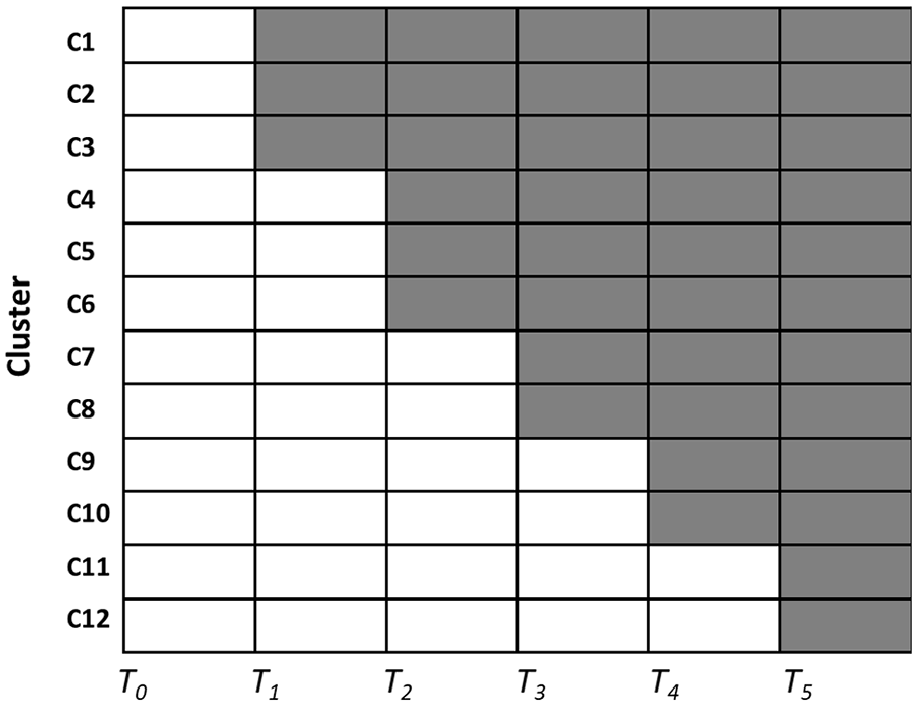
Schematic of a standard stepped-wedge design. Clusters are randomly allocated to transition from delivery of the standard of care (white cells) to delivery of the new intervention (gray cells) at different time points (T₁, T₂,…, T₅).

One important feature of the SW-CRT design is that early in the trial, participants predominantly receive the control treatment while late in the trial, they predominantly receive the new intervention. As a result, treatment received and time are correlated by design so time will be a confounder of the intervention–outcome relationship if there is an effect of time on the outcome, and analytic models that ignore this correlation will yield biased intervention effect estimates, as noted by Hussey and Hughes in their seminal paper. ¹ Other authors have argued that when the duration of the trial is short, the time effect is likely to be unimportant and it may be reasonable to ignore it. ⁹ Nonetheless, current consensus guidelines recommend that analyses should adjust for time effects to avoid the risk of bias. ¹⁰ Consequently, the power/sample size calculations used in designing a trial should also be based on an analytic model that includes time effects.

Within the Frequentist framework, the required sample size is substantially larger when the calculation accounts for time effects than when time effects are ignored, because adjusting for a variable (time, in this case) that is highly correlated with the intervention greatly increases the standard error of the intervention effect and so reduces the ability of the analysis to detect that effect.^11–13 Zhou et al. ¹⁴ compared models for continuous outcomes in the SW-CRT design with and without time effects, and found that the design incorporating time effects often required more than twice as many clusters as the one without time effects. Similarly, Baio et al. ¹⁵ concluded that failure to account for time effects at the design stage while including them at the analysis stage may artificially and grossly overestimate the power of a study. Adopting the sample size calculation that includes time effects would ensure the trial having adequate power regardless of the strength of the effect of time on the outcome. But if in fact time effects were negligible, this would overestimate the required sample size and could lead to the trial being deemed infeasible due to cost or unavailability of the required number of clusters or participants.

In some situations, prior information on the magnitudes of the time effects may be available, such as from historical trends in outcomes under the current standard of care. Or the expected change in outcome rates over time during the trial may be judged to be small if the trial is completed in relatively short time frame. The concern is perhaps not so much whether prior information is available (which it usually is, in our experience), but the extent to which the prior information is deemed informative of the time trends that will be encountered in the trial. Consideration of this information could enable trial designers to show that the trial would be adequately powered with a smaller sample size, potentially turning an infeasible trial into a feasible one. The Frequentist sample size calculation methods provide no option for making this assessment. We propose using a Bayesian model to incorporate this prior information in the design and analysis to narrow the uncertainty in the estimated time effects. This, in turn, would narrow the uncertainty in the estimated intervention effect and improve the efficiency of the trial while still adjusting for potential time effects.

This article provides a proof-of-principle illustration of the potential impact of incorporating priors for time effects on the bias in the intervention effect estimate and on trial power/sample size by presenting the numerical results from an example design that assumes linear time effects. The expectation is that when the means on the time effects priors match their true values, trial power will be increased while retaining unbiased estimates for the intervention effect, but mis-specification of these means can lead to biased estimates for the intervention effect. Through comparison to the Frequentist sample size calculations, we illustrate how incorporating prior information on time effects can address the shortcomings of the Frequentist power calculations and enable us to obtain a justifiable and accurate assessment of the required sample size. R code for continuous, binary, and count outcome models is included in the Supplementary material to assist researchers with exploring the utility of this approach for their own trial designs.

Methods

Bayesian stepped-wedge model

For expository concreteness, we illustrate our method using a slightly modified version of the Bayesian model used by Cunanan et al. ¹⁶ for the stepped-wedge design with a count outcome analyzed at the cluster level. Our model includes an intercept parameter to allow for estimation of the baseline outcome rate rather than pre-specifying the expected outcome rate. The models for continuous (Gaussian) and binary outcomes are described in the Supplementary material. Suppose the trial enrolls N _{i j} patients in cluster i (i = 1, …, I) during time period j (j = 1, …, J). Each patient contributes a single count outcome. Let Y _{i j} be the cluster-level count outcome aggregated over the N _{i j} patients in cluster i and time period j. We assume the Y _{i j} are independent Poisson (λ _{i j} ) random variables, where λ _{i j} is determined by

$$\log ({\lambda }_{\mathrm{ij}})=\log (N_{\mathrm{ij}})+\alpha +{\alpha }_i+{\beta }_j+\theta X_{\mathrm{ij}}$$

Here, $\alpha$ is the individual-level log-baseline rate in the population, α _i is the random effect for cluster i, β _j is the fixed time effect in period j, X _{i j} is the treatment group indicator (0 = control, 1 = intervention), and θ is the log-relative risk of an event for treatment versus control.

Cunanan et al. assumed that each cluster transitioned at equally spaced, unique time points (i.e. the number of periods equals the number of clusters plus one). Using simulation, they evaluated the (Frequentist) power and Type I error performance (i.e. the proportions of simulations that declare the intervention is effective when in fact it is not or it is true, respectively) ¹⁷ under the assumption of relatively flat prior distributions for the cluster random effects and the fixed time effects. Specifically, they assumed that α _i ∼ Normal (0, 1/τ²) where τ²∼ Gamma (0.1, 1) and that β _j ∼ Normal (0, 10), where Normal (a, b) denotes the normal distribution with mean a and variance b. For the intervention effect, they assumed a modestly informative prior, θ∼ Normal (0, 0.1), which assigns roughly 95% of the probability for θ in the interval (−0.63, 0.63). The intervention was declared to be effective if the posterior probability of a beneficial intervention effect was greater than 0.95, that is, if Pr (θ < 0| data) > 0.95. Their results suggested that the power and bias in the estimated intervention effect was relatively insensitive to the true values of the cluster effects variance and the time effects. However, they did not explore the impact of using an informative prior distribution on the time effects. In our work, we assumed a flatter prior for the cluster random effects, that is, α _i ∼ Normal (0, 1/τ²) where τ²∼ Gamma (0.001, 0.001) to ensure the intervention effect estimates would not be impacted by prior information for α _i . We also adopted nearly flat priors, $\alpha$ ∼ Normal (0, 100) and θ∼ Normal (0, 9), for the individual-level log-baseline rate and intervention effect, respectively. We investigated the impact of assuming priors with varying degrees of informativeness for the time effects β _j ∼ Normal (0, σ²) by varying the value of the prior standard deviation σ within the set of values (0.01, 0.05, 0.15, 0.3, 0.5, 3). To facilitate comparison with the standard Frequentist calculations that use a two-tailed test at significance level 0.05, we declared a difference between the two treatments if the Pr (θ < 0| data) > 0.975 or Pr (θ > 0| data) > 0.975.

Simulation study

To assess the performance of our models, we simulated trials assuming a true relative risk of 0.7 (i.e. θ≈−0.357 and a lower count corresponds to a better outcome). With respect to this magnitude for the intervention effect, the values of σ could be interpreted as follows: The value σ = 0.01 corresponds to nearly a point prior which represents near certainty regarding the magnitudes of the time effects (zero in this example) while the value σ = 3 corresponds to a nearly flat prior and represents very high uncertainty about the magnitudes of the time effects. The values in between could be interpreted roughly as “some uncertainty exists regarding the magnitudes of the time effects but the level of uncertainty is:” (a) σ = 0.05, “almost surely less than the intervention effect,” (b) σ = 0.15, “very likely less than the intervention effect,” (c) σ = 0.3 or 0.5 “similar to the magnitude of the intervention effect.” We set the true cluster effect variance at 1/τ² = 0.25, the individual-level log-baseline rate at $\alpha$  = 0.1175 and the cluster-period sizes at a constant value of N _{i j}  = 20. We fixed the number of transition steps at five to ensure that variation in our results could not be attributed to variation in the number of periods (that occur when the number of clusters changes, as was done in Cunanan et al.). If the number of the clusters was a multiple of five, then an equal number of clusters was allocated to transition at each step. Otherwise, the remaining clusters were assigned, for simplicity, to the transition steps sequentially beginning with the first step. For example, Figure 1 illustrates this scheme for a stepped wedge design with 12 clusters. After allocating two clusters to transition at each of the five steps, the remaining two clusters were allocated randomly to the first two steps. Thus, three clusters will transition at each of the first two steps, while two clusters will transition at each of the remaining steps. Note that changing the steps at which these remaining clusters transition would lead to a slightly different power, ¹⁸ which could change slightly the number of clusters needed, but this difference is immaterial to the ideas presented in this article.

In our base scenario, for each value of σ, we determined via simulation the minimum number of clusters required to obtain at least 80% power under the assumption that there were no time effects (i.e. the data were generated assuming β _j  = 0 for all time periods j). The number of simulation replicates was 8000 for each configuration of input parameter values, yielding a standard error of approximately 0.005 in the power estimates. The minimum number of clusters required was determined by making an initial guess and then adjusting that number through trial-and-error power calculations until the target power was achieved. In this scenario, the priors for the time effect were correctly specified in that they are centered around the true values of β _j . We assessed the gain in efficiency by comparing these sample sizes to the Frequentist calculation based on the generalized linear mixed model proposed by Hussy and Hughes ¹ using the simulation-based approach in the R package “SWSamp.”^15,19

As with all Bayesian analyses that utilize informative priors, a mis-specified prior may increase the bias of estimators so it is important to investigate the sensitivity of the results to the prior. Hence, in our sensitivity scenarios, we assumed the sample sizes calculated in the base scenario and evaluated the bias in estimating the intervention effect, defined as the posterior mean of θ, and the corresponding power as a function of the magnitude of mis-specification in the prior mean for the time effects (i.e. due to being not centered around the true values of β _j ). In practice, the relevant patterns and magnitudes of mis-specification that should be explored will vary with context. For illustrative purposes in this article, the time effects were assumed to be linear, with “small” (range of values of β _j  = θ/20), “medium” (range of β _j  = θ/10), “large” (range of β _j  = θ/4), and “very large” (range of β _j  = θ/2) magnitudes starting from 0 at baseline. Investigations were conducted for both increasing and decreasing outcome rates over time. The number of simulation replicates and all other model parameters were kept unchanged from the base scenario. Computations were conducted using the code published by Cunanan et al., with adaptations needed to match our models (see Supplementary materials). All simulations were done using RJAGS (version number 4.3.0) by R (version 3.6.1) on the Cedar Compute Canada computing cluster located at Simon Fraser University. Additional information about Markov Chain Monte Carlo settings and diagnostics can be found in the web appendix.

Results

Efficiency gain using an informative prior for the time effects, with correctly specified prior means

In the base scenario (no time effects/correctly specified prior means), the second row in Table 1 displays the minimum number of clusters needed to obtain at least 80% power (confirmed by the entries in the middle row labeled “None” in Table 2). The results suggested that even relatively modest knowledge about the time effects reduced substantially the number of clusters needed. When the prior was nearly flat (σ = 3), the required number of clusters was 51, which matched the result of the Frequentist calculation based on the model that included time effects. If σ was lowered to 0.3, corresponding to an uncertainty in the time effect similar in magnitude to the intervention effect (θ = −0.357), the required number of clusters decreased to 43. This number further decreased to 32 when σ was lowered to 0.15, which was roughly half of the intervention effect. And finally, when σ = 0.01, corresponding to the case where the designer knows the magnitudes of the time effects with near certainty, the required number of clusters decreased to 22, which matched the Frequentist result based on a model that omitted time effects.

Table 1.

Impact of the prior distribution for the time effects on the bias of the intervention effect (relative risk) estimate.

Standard deviationof the time effect prior (σ)		3	0.5	0.3	0.15	0.05	0.01

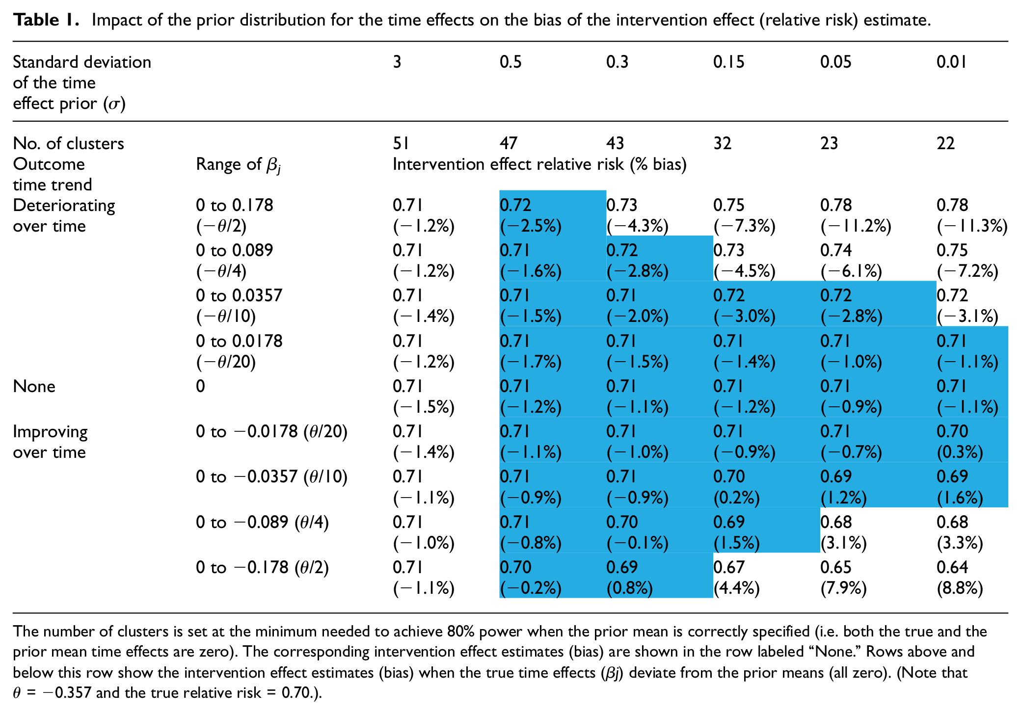
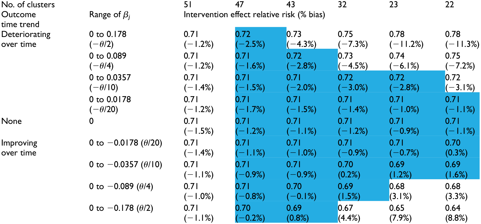
The number of clusters is set at the minimum needed to achieve 80% power when the prior mean is correctly specified (i.e. both the true and the prior mean time effects are zero). The corresponding intervention effect estimates (bias) are shown in the row labeled “None.” Rows above and below this row show the intervention effect estimates (bias) when the true time effects (β j) deviate from the prior means (all zero). (Note that θ = −0.357 and the true relative risk = 0.70.).

Table 2.

The impact of the prior distribution for the time effects on the trial power.

Standard deviation of the time effect prior (σ)		3	0.5	0.3	0.15	0.05	0.01

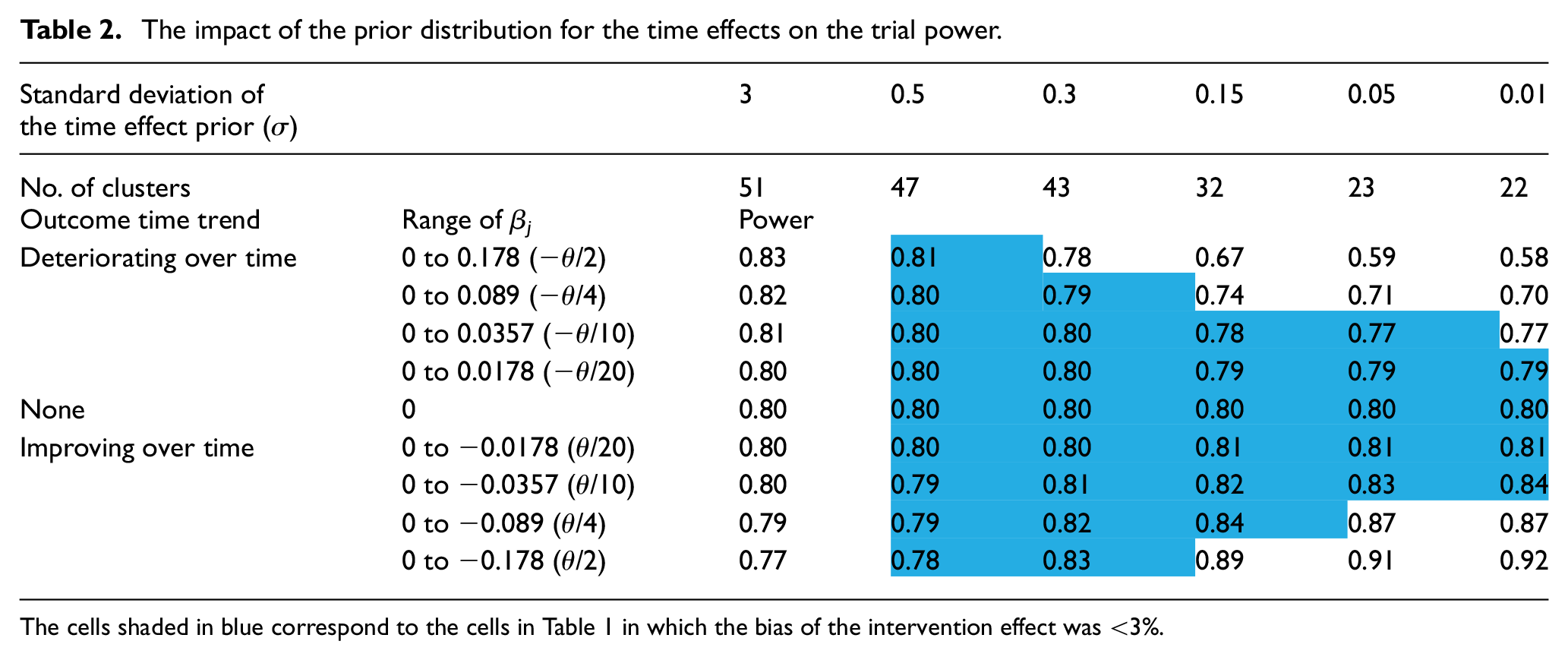
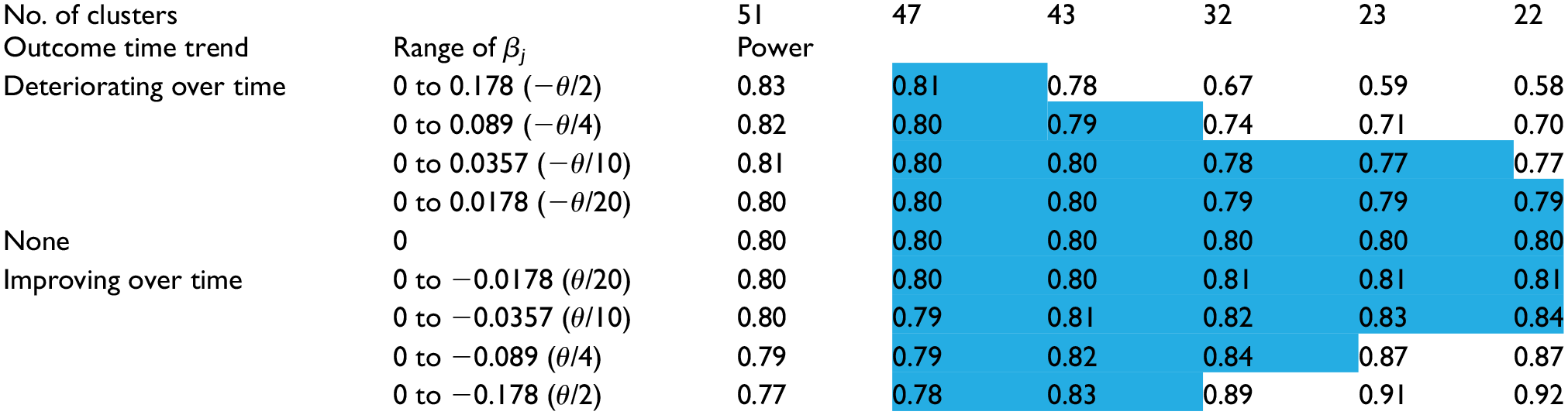
The cells shaded in blue correspond to the cells in Table 1 in which the bias of the intervention effect was <3%.

Across all of these choices for σ, we observed a small (∼1%) but relatively stable bias toward the null for the intervention effect on the relative risk scale (see the row labeled “None” in Table 1).

Bias due to mis-specification of the prior means of the time effects

The intervention effect estimates (bias) and the power under the sensitivity scenarios (linear time effect/mis-specified prior means) are shown in the four rows above and four rows below the row labeled “None” in Tables 1 and 2, respectively. When a nearly flat prior (σ = 3) was used, the intervention effect bias under different magnitudes of mis-specification all matched the values from the base scenario, which is consistent with the intuition that the prior mean is unimportant when the prior is nearly flat. However, the power decreased (increased) modestly when the outcome rate decreased (increased) over time. This result is not a feature of the Bayesian approach but is simply a consequence of the absolute difference in the outcome rates decreasing (increasing) over time, resulting in decreased (increased) difficulty in detecting the intervention effect—the Frequentist calculations exhibited the same pattern.

As σ decreased, the bias in the intervention effect estimate increased. The prior mean of zero for the time effects biased the time effects estimates toward zero, increasingly so as σ decreased, and led to the intervention effect estimates absorbing the bias that was induced in the time effects estimates. In this example, when the true time trend was decreasing (i.e. from zero to negative values of β _j , and corresponding to improved outcomes over time), but not captured fully in the time effects estimates, the intervention effect was overestimated (bias > 0). Conversely, when the time trend was increasing (corresponding to poorer outcomes over time), the intervention effect was underestimated (bias < 0). The intervention effect bias reached up to 11% when the range of time effects equaled one-half the true intervention effect and a precise prior was used. However, within the ranges of values for σ and for the β _j values, there existed a triangular region (cells shaded blue in Table 1), comprising situations with either larger values of σ or smaller β _j values, within which using the prior reduced the required number of clusters, yet introduced very little bias (< 3%) in the intervention effect estimate.

The choice for σ also impacted the trial power, but in different directions depending on the direction of the time effects trend. When the time trend was decreasing (outcomes improving over time), the power increased as σ decreased due to both an increase in precision and overestimation of the intervention effect. When the time trend was increasing, the power decreased as σ decreased due to underestimation of the intervention effect (the impact of which was not fully mitigated by an increase in precision). Though the power values showed a slightly different pattern to that seen for the intervention effects/bias in Table 1, there was a corresponding triangular region (cells shaded blue in Table 2), closely overlapping the one seen in Table 1, within which using the corresponding prior did not appreciably impact the trial power. That is, scenarios in which the bias was low corresponded well with the scenarios in which the power remained near the nominal 80%.

Discussion

We have proposed a Bayesian approach for calculating the number of clusters needed in a stepped-wedge trial that utilizes prior information about the magnitudes of the time effects and illustrated how this approach bridges the large difference in the number of required clusters that is obtained via the two Frequentist calculations when time effects are either included or ignored. The results show that when an informative time effects prior is used, this approach can reduce substantially the number of clusters needed, while introducing very little bias into the intervention effect estimate (and maintaining true power) as long as the prior time effects means are not greatly mis-specified. The robustness to modest mis-specification was particularly noteworthy—when the magnitude of mis-specification of the true time effects means was within roughly 10% of the intervention effect, the adoption of an informative prior, even one that was very precise, did not incur either substantial bias in the intervention effect estimate or a meaningful change in power. This result can be viewed as mathematical support for the argument that omitting time effects in the Frequentist design and analysis may be justified when the values of the time effects are assumed a priori to be known (often zero). However, claiming to know the time effects is a very strong assumption that we believe would be difficult to justify in practice. Hence, use of the Frequentist approach ignoring time effects or the analogous Bayesian approach in which near certainty in the time effects prior is assumed, should be avoided. As seen in the scenarios where the magnitudes of the time effects are not small compared to the intervention effect, mis-specification of the prior means of the time effects can lead to substantial bias in the intervention effect estimate and under-powering of the trial if the outcome time trend is worse than that assumed. We emphasize that the trial designer using the proposed Bayesian model must ensure that the choice of prior can be justified (such as having been obtained through a formal elicitation process with subject-area experts) and that it reflects the true uncertainty in the time effects. To ensure that the potential consequences of using a particular prior are well understood before setting the sample size, we recommend the trial designer assess the sensitivity of the trial performance characteristics to the true time effects (as exemplified in Tables 1 and 2), as well as compare to case where an uninformative prior is assumed.

We observed similar patterns in the results for our examples with continuous and binary outcomes, although for the continuous outcome, changes in the magnitudes of the true time effect did not affect the power values, since the difference in mean outcomes between the two interventions does not depend on the time effects (see Supplementary materials for details). For binary or count outcomes, if there is need to mitigate the change in power due to the presence of the time trend when designing a specific trial, the designer can replace the individual-level baseline outcome rate with the expected outcome rate at the mid-point of the trial.

How often the proposed approach will find applicability in the real world remains unclear. The natural histories of most diseases evolve slowly, and when the standard of care has remained the same for some time, one would expect the outcome rates to change relatively slowly. Thus, historical time trends typically can be estimated fairly precisely, which suggests that this approach has the potential to be widely applicable. However, while considerable literature exists on the methods for eliciting priors for intervention effects, we are not aware of any prior elicitation work addressing the extrapolation of historical trends to a future trial. Because historical time trends may not persist into the future, a key risk to consider when deciding whether to adopt the proposed approach is that the approach would not be robust to disruptions in these trends.

Our results should be interpreted as a proof of principle demonstration in a limited range of settings. The scope of our simulation work necessarily was limited due to the many input parameters used in the power calculations, and considered only on the cross-sectional design. We expect that our main conclusions qualitatively would hold if the values of input parameters such as the treatment effect size, the number of time periods, and so on were to vary, but trial designers will need to conduct simulations using appropriate inputs to assess the magnitudes of the benefits and risks of applying this approach in their specific contexts. Due to the substantial computational time needed to conduct the simulations, development of analytic approximations would facilitate obtaining more general conclusions across more diverse scenarios, as well as making this method accessible. However, the simulation code is relatively simple and easy for trial designers to use, so ought to be adequate to meet the needs for a specific trial that utilizes a continuous, binary, or count outcome.

Our examples were restricted to designs with six periods and assumed a continuous, linear effect of time on (the transformed) outcomes. The performance of the proposed method for designs with different numbers of periods or for other time effect parameterizations has not yet been evaluated. Our code allows for setting and estimating the time effect in each period independently from other periods, though this parameterization of the time effects may not be the most appropriate or efficient one in general. Recent work by various groups have investigated the impact of parameterization and mis-specification of time effects on analytic validity and power within the Frequentist framework.^20–22 Future work could investigate these impacts within this Bayesian approach.

Because of the potential risks of introducing bias when prior distributions (for time trends as in this article, but more generally for other model parameters) are mis-specified, we do not recommend incorporating prior information as the default approach when calculating required sample sizes. An additional risk in this calculation is that the trial ultimately may be under-powered if it was determined later and that a less informative prior was appropriate at the data analysis stage. However, in situations where trial feasibility is jeopardized due to (lack of) availability of sufficient numbers of clusters or participants, incorporating external information on time effects using this Bayesian approach enables assessment of whether a smaller sample size could be adequate and so can better inform the decision about whether the trial should be conducted.

Supplemental Material

sj-pdf-1-ctj-10.1177_1740774520980052 – Supplemental material for Improving efficiency in the stepped-wedge trial design via Bayesian modeling with an informativeprior for the time effects

Supplemental material, sj-pdf-1-ctj-10.1177_1740774520980052 for Improving efficiency in the stepped-wedge trial design via Bayesian modeling with an informativeprior for the time effects by Denghuang Zhan, Yongdong Ouyang, Liang Xu and Hubert Wong in Clinical Trials

Supplemental Material

sj-pdf-2-ctj-10.1177_1740774520980052 – Supplemental material for Improving efficiency in the stepped-wedge trial design via Bayesian modeling with an informativeprior for the time effects

Supplemental material, sj-pdf-2-ctj-10.1177_1740774520980052 for Improving efficiency in the stepped-wedge trial design via Bayesian modeling with an informativeprior for the time effects by Denghuang Zhan, Yongdong Ouyang, Liang Xu and Hubert Wong in Clinical Trials

Supplemental Material

sj-pdf-3-ctj-10.1177_1740774520980052 – Supplemental material for Improving efficiency in the stepped-wedge trial design via Bayesian modeling with an informativeprior for the time effects

Supplemental material, sj-pdf-3-ctj-10.1177_1740774520980052 for Improving efficiency in the stepped-wedge trial design via Bayesian modeling with an informativeprior for the time effects by Denghuang Zhan, Yongdong Ouyang, Liang Xu and Hubert Wong in Clinical Trials