A Bayesian adaptive design approach for stepped-wedge cluster randomized trials

Abstract

Background:

The Bayesian group sequential design has been applied widely in clinical studies, especially in Phase II and III studies. It allows early termination based on accumulating interim data. However, to date, there lacks development in its application to stepped-wedge cluster randomized trials, which are gaining popularity in pragmatic trials conducted by clinical and health care delivery researchers.

Methods:

We propose a Bayesian adaptive design approach for stepped-wedge cluster randomized trials, which makes adaptive decisions based on the predictive probability of declaring the intervention effective at the end of study given interim data. The Bayesian models and the algorithms for posterior inference and trial conduct are presented.

Results:

We present how to determine design parameters through extensive simulations to achieve desired operational characteristics. We further evaluate how various design factors, such as the number of steps, cluster size, random variability in cluster size, and correlation structures, impact trial properties, including power, type I error, and the probability of early stopping. An application example is presented.

Conclusion:

This study presents the incorporation of Bayesian adaptive strategies into stepped-wedge cluster randomized trials design. The proposed approach provides the flexibility to stop the trial early if substantial evidence of efficacy or futility is observed, improving the flexibility and efficiency of stepped-wedge cluster randomized trials.

Introduction

Adaptive design strategies that make adjustments based on accumulating data have received extensive attention in clinical research due to improved flexibility, efficiency, and ethics. ¹ They enable researchers to modify design in the middle of a trial based on interim observations, without destroying the validity and integrity of intended studies. ² One of the popular adaptive strategies is the group sequential design, which employs stopping rules that allow researchers to decide whether to stop a trial early in case of overwhelming evidence of efficacy or futility based on interim data. ³ This strategy potentially can enhance flexibility and reduce patient exposure, cost, and trial duration.

Within the Bayesian paradigm, the Bayesian group sequential design has been investigated by many researchers.^4–6 It can, like traditional group sequential designs, stop the trial early due to efficacy or futility, but with its own advantages: (1) it provides a natural way to use information from previous studies or clinicians’ opinion; (2) it obeys the likelihood principle and does not require the large sample theory for valid inference; (3) it offers results interpretable through a decision theoretical framework. ⁷ Many researchers have advocated that Bayesian trial designs be calibrated to have good frequentist properties.^8–11 One important argument is that researchers and regulatory agencies care about the long-run behavior of a trial design, averaged over all therapies evaluated, which is inherently a frequentist outlook. In this spirit, and in adherence to regulatory practice, a Food and Drug Administration ¹² (FDA) guideline has recommended to assess frequentist operating characteristics, such as type I error and power for Bayesian trial designs. There has been rich development in the design of Bayesian adaptive trials primarily based on frequentist operating characteristics.^13–15

Recently, stepped-wedge cluster randomized trials (SW-CRTs) have been increasingly used in large biomedical and health care studies.^16–18 In a standard SW-CRT, clusters are randomized to different sequences, which all begin with the control but crossover to the experimental intervention at different steps. At the final step, all clusters receive intervention. Outcome measurements are collected at each step.^19,20 SW-CRTs have been preferred in pragmatic studies due to several advantages. It allows stepwise introduction of interventions to all clusters, which mitigates the ethical dilemma of withholding an intervention believed to be superior to the control. It helps reduce logistical challenges, especially when it is difficult to initiate the intervention concurrently to all subjects due to practical or financial constraints. It provides a fair and ethical random process to determine who receive the intervention first as long as all clusters receive the intervention within a reasonable time frame. ²¹ Finally, measurements over multiple steps offer insights into the temporal trend of the intervention effect.

Importantly, the stepwise crossover to intervention and longer study duration motivate the implementation of Bayesian adaptive design strategies. For example, when overwhelming evidence of futility or efficacy is observed at interim analysis, it might be desirable to stop the SW-CRT early to save time and resources. ³ Reaching the conclusion early also accelerates adoption by general practice. The Bayesian approach also enables knowledge from previous studies and researchers’ professional opinions to be incorporated into study design through the specification of informative priors. In summary, combining SW-CRTs with Bayesian adaptive strategies has great potential to improve experimental design methodologies and trial practice for pragmatic studies.

Development of adaptive methods for SW-CRTs has been scarce. Grayling et al. ³ presented a frequentist group sequential approach for SW-CRTs using the error spending method. There have been some applications of Bayesian models to analyze data generated from SW-CRTs.^22,23 Cunanan et al. ²⁴ presented a non-adaptive Bayesian SW design for community-based cluster randomized trials. Zhan et al. ²⁵ investigated how informative priors specified on time effects in SW-CRTs impact bias and efficiency. To the best of our knowledge, there has been no development of Bayesian adaptive design methods for SW-CRTs.

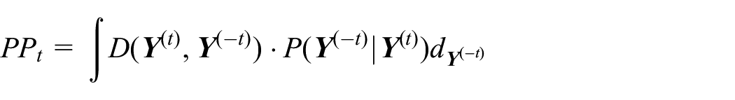
In this study, we proposed a Bayesian adaptive approach for SW-CRTs based on posterior predictive probabilities (PPP), which examines accumulating data at interim to determine whether the trial should be stopped early due to overwhelming efficacy/futility or should continue. By constructing decision rules based on PPP, the proposed adaptive design mimics typical clinical decision-making processes. Specifically, conditioning on interim data, the chance (predictive probability) that the trial will demonstrate a conclusive result at the planned end of study is evaluated. The decision to continue or to stop is made according to the strength of this predictive probability, examined against pre-specified thresholds. Extensive simulations are performed to determine various design parameters, so frequentist trial properties (e.g. type I error and power) are preserved.

This article is organized as follows. In “Methods” section, we describe the Bayesian adaptive approach for cross-sectional SW-CRTs and its implementation details. In “Results” section, we conduct extensive simulations to examine how the design parameters and different combinations of thresholds influence the design properties, such as power, type I error, and expected number of subjects. We also illustrate the proposed method with a real example. In “Conclusion” section, we summarize the proposed method and discuss practical issues.

Methods

We describe the Bayesian adaptive approach in the context of a cross-sectional SW-CRT, which could be readily extended to closed-cohort SW-CRTs. A typical SW-CRT involves $T$ steps (time points) and $n$ clusters. All clusters start from control, and they are randomized to switch to intervention at step $t(t=2,\dots ,T)$ and remain on intervention until the end of study, resulting in $S=(T-1)$ sequences. Let $p_s$ be the probability of a cluster being randomly assigned to sequence ${\mathit{v}}_s=(v_{s1},\dots ,v_{\mathit{sT}})\prime$ with $\sum _{s=1}^S{p}_s=1$ , where ${\mathit{v}}_s$ is defined so that its elements $v_{\mathit{st}}=0$ for $t=1,\dots ,s$ and $v_{\mathit{st}}=1$ for $t=s+1,\dots ,T$ . Here, value 0/1 indicates control/intervention. At step $t$ , a new panel of $J$ subjects is enrolled from Cluster $i(i=1,\dots ,n)$ . We assume each subject to contribute one outcome measurement. The total number of subjects enrolled is $N=\mathit{nJT}$ . Let $Y_{\mathit{ijt}}$ be the measurement of a continuous outcome obtained at step $t(t=1,\dots ,T)$ from subject $j(j=1,\dots ,J)$ of the $i\mathrm{th}$ cluster $(i=1,\dots ,n)$ . Under the Bayesian framework, we model the likelihood of $Y_{\mathit{ijt}}$ by

$$Y_{\mathit{ijt}}|{\lambda }_t,\zeta ,{\alpha }_i,{\gamma }_{\mathit{it}},{\sigma }_e^2~N({\lambda }_t+u_{\mathit{it}}\zeta +{\alpha }_i+{\gamma }_{\mathit{it}},{\sigma }_e^2)$$

(1)

with

$${\alpha }_i|{\sigma }_C^2~N(0,{\sigma }_C^2)\mathrm{and}{\gamma }_{\mathit{it}}|{\sigma }_{\mathit{CP}}^2~N(0,{\sigma }_{\mathit{CP}}^2)$$

Here $\mathbf{\lambda }=({\lambda }_1,\dots ,{\lambda }_T)\prime$ are time-specific intercepts, which account for arbitrary temporal trends under control. We use $u_{\mathit{it}}=0/1$ to indicate that cluster $i$ receives control/intervention at step $t$ and $\zeta$ quantifies the intervention effect. Define ${\mathit{u}}_i=(u_{i1},\dots ,u_{\mathit{iT}})\prime$ . By randomization, $P({\mathit{u}}_i={\mathit{v}}_s)=p_s$ . This model includes ${\alpha }_i$ as the cluster random effect and ${\gamma }_{\mathit{it}}$ as the cluster-period random effect, which are assumed to be mutually independent. Similar models have been employed by other researchers.^26,27 The correlation between measurements from the same cluster within the same period, called the within-period intracluster correlation (wpICC), is ${\rho }_1=\frac{{\sigma }_C^2+{\sigma }_{\mathit{CP}}^2}{{\sigma }_C^2+{\sigma }_{\mathit{CP}}^2+{\sigma }_e^2}$ . The correlation between measurements from the same cluster but across different periods, called the between-period intracluster correlation (bpICC), is ${\rho }_2={\rho }_{1}r$ $(0\le r\le 1)$ , where $r=\frac{{\sigma }_C^2}{{\sigma }_C^2+{\sigma }_{\mathit{CP}}^2}$ has been called the cluster autocorrelation coefficient (CAC). ²⁶ Importantly, the within-cluster correlations of $Y_{\mathit{ijt}}\mathrm{\prime }\mathrm{s}$ are exchangeable across steps under $r=1$ , and block exchangeable (by steps) otherwise. ²⁷

At step $t$ , the cluster-specific collection of observations is ${\mathit{Y}}_{\mathit{it}}=(Y_{i1t},\dots ,Y_{\mathrm{iJt}})\prime$ and we define ${\mathit{Y}}_t=({\mathit{Y}\prime }_{1t},\dots ,{\mathit{Y}\prime }_{\mathit{nt}})\prime$ . We use ${\mathit{Y}}^{(t)}={({\mathit{Y}\prime }_1,\dots ,{\mathit{Y}\prime }_t)}^{\prime }$ to denote interim observations up to step $t$ . Hence, the full set of observations at the end of study is ${\mathit{Y}}^{(T)}$ . For $1\le t<T$ , we have

$${\mathit{Y}}^{(T)}={\mathit{Y}}^{(t)}\cup {\mathit{Y}}^{(-t)}$$

where ${\mathit{Y}}^{(-t)}={({\mathit{Y}\prime }_{t+1},\dots ,{\mathit{Y}\prime }_T)}^{\prime }$ represents future observations yet to be observed at step $t$ .

To facilitate discussion, we rewrite Model (1) in a matrix form

$${\mathit{Y}}_t|{\mathit{\beta }}_1,{\mathit{\beta }}_2,{\mathit{\beta }}_3,{\sigma }_e^2~N({\mathit{X}}_{1t}{\mathit{\beta }}_1+{\mathit{X}}_{2t}{\mathit{\beta }}_2+{\mathit{X}}_{3t}{\mathit{\beta }}_3,{\sigma }_e^2{\mathit{I}}_{\mathit{nJ}})$$

(2)

We define ${\mathit{\beta }}_1=(\mathbf{\lambda }\mathbf{\prime },\zeta )\prime$ , ${\mathit{\beta }}_2=({\alpha }_1,\dots ,{\alpha }_n)\prime$ , ${\mathit{\beta }}_3=({\mathbf{\gamma }\mathbf{\prime }}_1,\dots ,{\mathbf{\gamma }\mathbf{\prime }}_T)\prime$ with ${\mathbf{\gamma }\mathbf{\prime }}_t=({\gamma }_{1t},\dots ,{\gamma }_{\mathit{nt}})\prime$ for $t=1,\dots ,T$ . ${\mathit{I}}_{\mathit{nJ}}$ is an $\mathit{nJ}\times \mathit{nJ}$ identity matrix. ${\mathit{X}}_{1t}$ is an $\mathit{nJ}\times (T+1)$ design matrix where the row corresponding to $Y_{\mathit{ijt}}$ is a vector with the $t\mathrm{th}$ element being 1, the $(T+1)\mathrm{th}$ element being $u_{\mathit{it}}$ , and all other elements being 0. ${\mathit{X}}_{2t}$ is an $\mathit{nJ}\times n$ design matrix for cluster random effects, where the row corresponding to $Y_{\mathit{ijt}}$ is a vector with the $i\mathrm{th}$ element being 1 and all others being 0. ${\mathit{X}}_{3t}$ is an $\mathit{nJ}\times \mathit{nT}$ design matrix for cluster-period random effects, where the row corresponding to $Y_{\mathit{ijt}}$ is a vector with the $[(i-1)T+i]\mathrm{th}$ element being 1 and all other elements being 0. Note that $\{({\mathit{X}}_{1t},{\mathit{X}}_{2t},{\mathit{X}}_{3t}),t=1,\dots T\}$ are known after randomization. Finally, ${\mathit{X}}_1^{(t)}$ , ${\mathit{X}}_2^{(t)}$ , ${\mathit{X}}_3^{(t)}$ , ${\mathit{X}}_1^{(-t)}$ , ${\mathit{X}}_2^{(-t)}$ , and ${\mathit{X}}_3^{(-t)}$ are defined similarly as ${\mathit{Y}}^{(t)}$ and ${\mathit{Y}}^{(-t)}$ .

Prior distributions for ${\mathit{\beta }}_1$ , ${\mathit{\beta }}_2$ , ${\mathit{\beta }}_3$ , and ${\sigma }_e^2$ need to be specified. Model (1) implies that ${\mathit{\beta }}_2|{\sigma }_C^2~N(0,{\sigma }_C^2{\mathit{I}}_n)$ and ${\mathit{\beta }}_3|{\sigma }_{\mathit{CP}}^2~N(0,{\sigma }_{\mathit{CP}}^2{\mathit{I}}_{\mathit{nT}})$ . Fixed-effect ${\mathit{\beta }}_1$ is assumed a non-informative flat prior, which is equivalent to a normal distribution with an infinite variance. It can be shown that there is a deterministic relationship between $({\sigma }_e^2,{\sigma }_C^2,{\sigma }_{\mathit{CP}}^2)$ and $({\sigma }_e^2,{\rho }_1,r)$ . Because variances of random effects $({\sigma }_C^2,{\sigma }_{\mathit{CP}}^2)$ are rather abstract concepts, it is often easier to obtain information (from literature or professional opinion) about intracluster correlation $\left({\rho }_1\right)$ and decay of correlation between periods $\left(r\right)$ . Hence, we decide to specify priors on $({\sigma }_e^2,{\rho }_1,r)$ instead of $({\sigma }_e^2,{\sigma }_C^2,{\sigma }_{\mathit{CP}}^2)$ . Following Grantham et al., ²⁷ we assume Beta distributions for ${\rho }_1$ and $r$ , which have a range of 0–1, and a half-Cauchy distribution for ${\sigma }_e^2$ . Gelman ²⁸ showed that the half-Cauchy prior is superior to the inverse-gamma prior for variance parameters, which can severely distort inference.

The hypotheses of interest are $H_0:\zeta \le {\zeta }_0$ versus $H_1:\zeta >{\zeta }_0$ , where ${\zeta }_0$ is the benchmark intervention effect. Under the Bayesian paradigm, hypothesis testing is performed based on the posterior distribution of $\zeta$ . At the end of study, we will declare the intervention effective if $P(\zeta >{\zeta }_0|{\mathit{Y}}^{(T)})>{\theta }_U$ ; ineffective if $P(\zeta >{\zeta }_0|{\mathit{Y}}^{(T)})<{\theta }_L$ ; and the trial is inconclusive if ${\theta }_L\le P(\zeta >{\zeta }_0|{\mathit{Y}}^{(T)})\le {\theta }_U$ . Here, decision thresholds $({\theta }_L,{\theta }_U)$ are design parameters that need to be specified to achieve desired operating characteristics, such as power and type I error. At each step $t$ , given interim observations ${\mathit{Y}}^{(t)}$ , we will calculate the predictive probability (denoted by $P{P}_t$ ) of declaring the intervention effective at the end of study. We will use $P{P}_t$ to determine whether the trial should be stopped early due to overwhelming evidence of efficacy/futility, based on decision rules:

• If $P{P}_t<{\pi }_L$ , stop the trial and conclude the intervention ineffective;

• If $P{P}_t>{\pi }_U$ , stop the trial and conclude the intervention effective;

• Otherwise, continue to step $(t+1)$ until reaching the end of study.

The interim decision thresholds $({\pi }_L,{\pi }_U)$ also need to be specified.

In the following, we describe the evaluation of $P{P}_t$ . At the end of study, given fully observed data ${\mathit{Y}}^{(T)}={\mathit{Y}}^{(t)}\cup {\mathit{Y}}^{(-t)}$ , the decision function for declaring the intervention effective can be written as

$$D({\mathit{Y}}^{(t)},{\mathit{Y}}^{(-t)})=I\{P(\zeta >{\zeta }_0|{\mathit{Y}}^{(T)})>{\theta }_U\}$$

That is, we declare the intervention effective if $D({\mathit{Y}}^{(t)},{\mathit{Y}}^{(-t)})=1$ . At step $t$ , however, only ${\mathit{Y}}^{(t)}$ is observed, which prevents direct evaluation of $D({\mathit{Y}}^{(t)},{\mathit{Y}}^{(-t)})$ . We propose to make interim decisions based on the predictive probability of rejecting $H_0$ given ${\mathit{Y}}^{(t)}$ ,

$$P{P}_t=\int D({\mathit{Y}}^{(t)},{\mathit{Y}}^{(-t)})·P({\mathit{Y}}^{(-t)}|{\mathit{Y}}^{(t)})d_{{\mathit{Y}}^{(-t)}}$$

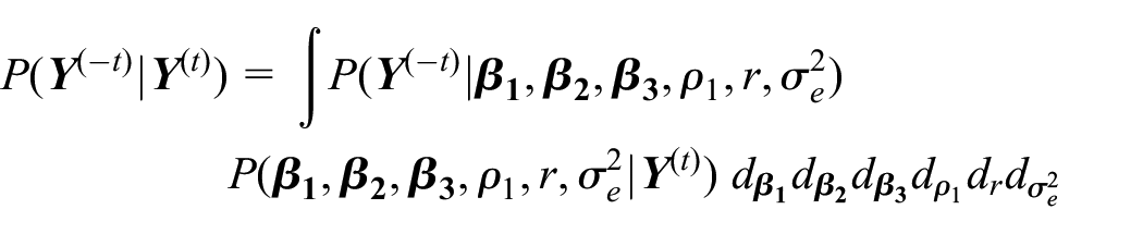
Here $P({\mathit{Y}}^{(-t)}|{\mathit{Y}}^{(t)})$ is the posterior predictive distribution of future observations ${\mathit{Y}}^{(-t)}$ given ${\mathit{Y}}^{(t)}$ . Specifically,

$$\begin{array}{c}P({\mathit{Y}}^{(-t)}|{\mathit{Y}}^{(t)})=\int P({\mathit{Y}}^{(-t)}|{\mathit{\beta }}_1,{\mathit{\beta }}_2,{\mathit{\beta }}_3,{\rho }_1,r,{\sigma }_e^2)\hfill \\ P({\mathit{\beta }}_1,{\mathit{\beta }}_2,{\mathit{\beta }}_3,{\rho }_1,r,{\sigma }_e^2|{\mathit{Y}}^{(t)})d_{{\mathit{\beta }}_1}{d}_{{\mathit{\beta }}_2}{d}_{{\mathit{\beta }}_3}{d}_{{\rho }_1}{d}_r{d}_{{\sigma }_e^2}\hfill \end{array}$$

where $P({\mathit{Y}}^{(-t)}|{\mathit{\beta }}_1,{\mathit{\beta }}_2,{\mathit{\beta }}_3,{\rho }_1,r,{\sigma }_e^2)$ is the predictive distribution and $P({\mathit{\beta }}_1,{\mathit{\beta }}_2,{\mathit{\beta }}_3,{\rho }_1,r,{\sigma }_e^2|{\mathit{Y}}^{(t)})$ is the posterior distribution of model parameters given ${\mathit{Y}}^{(t)}$ .

Because distributions such as $P({\mathit{Y}}^{(-t)}|{\mathit{Y}}^{(t)})$ and $P({\mathit{\beta }}_1,{\mathit{\beta }}_2,{\mathit{\beta }}_3,{\rho }_1,r,{\sigma }_e^2|{\mathit{Y}}^{(t)})$ do not have a closed form, the evaluation of $P{P}_t$ is accomplished through a series of numerical integration.

First, based on interim observations ${\mathit{Y}}^{(t)}$ , we generate $L$ random samples from posterior distribution $P({\mathit{\beta }}_1,{\mathit{\beta }}_2,{\mathit{\beta }}_3,{\rho }_1,r,{\sigma }_e^2|{\mathit{Y}}^{(t)})$ through Markov Chain Monte Carlo (MCMC) simulation.

Second, plug the posterior samples obtained from the first step into $P({\mathit{Y}}^{(-t)}|{\mathit{\beta }}_1,{\mathit{\beta }}_2,{\mathit{\beta }}_3,{\rho }_1,r,{\sigma }_e^2)$ and generate future observations (denoted by ${\hat{\mathit{Y}}}^{(-t)}$ ) from distribution $P({\mathit{Y}}^{(-t)}|{\mathit{\beta }}_1,{\mathit{\beta }}_2,{\mathit{\beta }}_3,{\rho }_1,r,{\sigma }_e^2)$ . Let $\{{\hat{\mathit{Y}}}^{(-t),l},l=1,\dots ,L\}$ be $L$ samples of ${\hat{\mathit{Y}}}^{(-t)}$ generated.

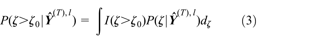
Third, we treat ${\hat{\mathit{Y}}}^{(T),l}={\mathit{Y}}^{(t)}\cup {\hat{\mathit{Y}}}^{(-t),l}$ as a “full” dataset. Then, $P{P}_t$ is numerically obtained as the average of $D({\mathit{Y}}^{(t)},{\hat{\mathit{Y}}}^{(-t),l})$ over $l=1,\dots ,L$ . Importantly, the value of $D({\mathit{Y}}^{(t)},{\hat{\mathit{Y}}}^{(-t),l})$ is determined by

$$P(\zeta >{\zeta }_0|{\hat{\mathit{Y}}}^{(T),l})=\int I(\zeta >{\zeta }_0)P(\zeta |{\hat{\mathit{Y}}}^{(T),l})d_{\zeta }$$

(3)

Here $P(\zeta |{\hat{\mathit{Y}}}^{(T),l})$ is the marginal posterior distribution of $\zeta$ given ${\hat{\mathit{Y}}}^{(T),l}$ , obtained from the joint posterior distribution $P({\mathit{\beta }}_1,{\mathit{\beta }}_2,{\mathit{\beta }}_3,{\rho }_1,r,{\sigma }_e^2|{\hat{\mathit{Y}}}^{(T),l})$ . In practice, for every sample ${\hat{\mathit{Y}}}^{(-t),l}$ , the evaluation of equation (3) requires a separate numerical integration based on MCMC simulation from $P({\mathit{\beta }}_1,{\mathit{\beta }}_2,{\mathit{\beta }}_3,{\rho }_1,r,{\sigma }_e^2|{\hat{\mathit{Y}}}^{(T),l})$ .

The detailed algorithm to conduct a Bayesian adaptive SW-CRT based on the monitoring of $\mathrm{PP}$ is described below. After randomization based on $P({\mathit{u}}_i={\mathit{v}}_s)=p_s$ , define ${\mathit{u}}^{(t)}=(u_{1t},\dots ,u_{\mathit{nt}})\prime$ , which indicates the treatments received by clusters at step $t(t=1,\dots ,T)$ . It has been recommended to start the Bayesian adaptive scheme after enough data have been collected to avoid premature decisions due to spurious results.^5,29 We assume that adaptation starts from step $t_0,1<t_0<T$ .

Algorithm 1

1. At step $t(t_0\le t<T)$ , obtain interim observation ${\mathit{Y}}^{(t)}$ based on ${\mathit{u}}^{(t)}$ and other design parameters. For the $l\mathrm{th}(l=1,\dots ,L)$ iteration,

2. (b) Generate a sample of future observation ${\mathit{Y}}^{(-t)}$ from $P({\mathit{Y}}^{(-t)}|{\mathit{Y}}^{(t)})$ , denoted by ${\hat{\mathit{Y}}}^{(-t),l}$ .

3. (c) Construct a “full” dataset ${\hat{\mathit{Y}}}^{(T),l}={\mathit{Y}}^{(t)}\cup {\hat{\mathit{Y}}}^{(-t),l}$ . Generate $Q$ samples of $({\mathit{\beta }}_1,{\mathit{\beta }}_2,{\mathit{\beta }}_3,{\rho }_1,r,{\sigma }_e^2)$ from $P({\mathit{\beta }}_1,{\mathit{\beta }}_2,{\mathit{\beta }}_3,{\rho }_1,r,{\sigma }_e^2|{\hat{\mathit{Y}}}^{(T),l})$ . The samples are denoted by $\{({\hat{\mathit{\beta }}}_1^q,{\hat{\mathit{\beta }}}_2^q,{\hat{\mathit{\beta }}}_3^q,{\hat{\mathit{\beta }}}_1^q,{\hat{r}}^q,{\hat{\sigma }}_e^{2,q}),q=1,\dots ,Q\}$ . Here, we use accent ∧ to indicate that the samples are generated using simulated future observations ${\hat{\mathit{Y}}}^{(-t),l}$ .

4. (d) Numerically evaluate $P(\zeta >{\zeta }_0|{\hat{\mathit{Y}}}^{(T),l})\approx \frac{1}{Q}\sum _{q=1}^{Q}I({\hat{\zeta }}^q>{\zeta }_0)$ . Note that ${\hat{\zeta }}^q$ is the $(T+1)\mathrm{th}$ element of ${\hat{\mathit{\beta }}}_1^q$ .

5. (e) Obtain $D({\mathit{Y}}^{(t)},{\hat{\mathit{Y}}}^{(-t),l})=I\{P(\zeta >{\zeta }_0|{\hat{\mathit{Y}}}^{(T),l})>{\theta }_U\}$ .

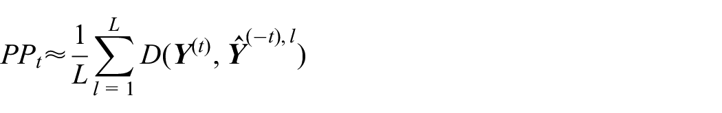
The predictive probability of declaring the intervention effective at the end of study is numerically evaluated by

$$P{P}_t\approx \frac{1}{L}\sum _{l=1}^{L}D({\mathit{Y}}^{(t)},{\hat{\mathit{Y}}}^{(-t),l})$$

Make adaptive decisions:

(a) If $P{P}_t<{\pi }_L,$ stop the trial early and conclude the intervention ineffective;

(b) If $P{P}_t>{\pi }_U,$ stop the trial early and conclude the intervention effective;

(c) Otherwise, set $t=t+1$ . If $t\le T-1$ , go to #1. If $t=T$ , go to #4.

Stop the trial. Obtain full observation ${\mathit{Y}}^{(T)}$ .

(a) Generate $Q$ samples of $\zeta$ from posterior distribution $P({\mathit{\beta }}_1,{\mathit{\beta }}_2,{\mathit{\beta }}_3,{\rho }_1,r,{\sigma }_e^2|{\mathit{Y}}^{(T)})$ , denoted by $\{{\zeta }^q,q=1,\dots ,Q\}$ .

(b) Numerically evaluate $P(\zeta >{\zeta }_0|{\mathit{Y}}^{(T)})\approx \frac{1}{Q}\sum _{q=1}^{Q}I({\zeta }^q>{\zeta }_0)$ .

(c) If $P(\zeta >{\zeta }_0|{\mathit{Y}}^{(T)})>{\theta }_U,$ declare the intervention effective; if $P(\zeta >{\zeta }_0|{\mathit{Y}}^{(T)})<{\theta }_L$ , declare the intervention ineffective; otherwise, declare the trial inconclusive.

To simplify notations, we have assumed a constant cluster size $J$ . In practice, the numbers of patients enrolled from each cluster are likely to vary randomly across steps. To address this pragmatic issue, we define $J_{\mathit{it}}$ to be the number of enrolled patients from cluster $i$ at step $t$ , which is a discrete random variable with mean $J_m$ and variance $J_v$ . The total number of subjects is $N=\sum _{i=1}^n\sum _{t=1}^T{J}_{\mathit{it}}$ . Extension of the above models and algorithms to random cluster sizes $J_{\mathit{it}}$ is straightforward.

Results

Simulation studies

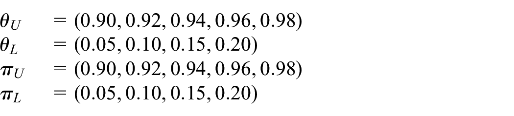
We conduct extensive simulations to illustrate the proposed Bayesian adaptive SW-CRT method and assess the relationship between design parameters (such as decision thresholds, number of clusters, and number of steps) and operating characteristics (such as type I error, power, and the probability of early stop). We assume a cross-sectional SW-CRT with $T=5$ time periods (hence $S=4$ ) and a constant cluster size $J=10$ . We specify time-specific intercepts ${\lambda }_t=0.1t$ , an evenly transitioning scheme with $p_s=\frac{1}{S}$ for $s=1,\dots ,S$ , wpICC with ${\rho }_1=0.05$ , an exchangeable correlation structure with $r=1$ , and ${\sigma }_e^2=1$ . The benchmark intervention effect is set at ${\zeta }_0=0$ . We explore the true values of intervention effect $\zeta$ from 0 to 0.3. We implement the Bayesian adaptive strategy from step $t_0=3$ .

To complete the design of a Bayesian adaptive SW-CRT, the number of clusters $\left(n\right)$ and decision thresholds $({\theta }_U,{\theta }_L,{\pi }_U,{\pi }_L)$ need to be specified. We conduct simulation studies to explore a range of specifications and select the configurations that achieve desired operational characteristics. For illustration, we explore $n=\{15,20,25\}$ and

$$\begin{array}{cc}{\theta }_U\hfill & =(0.90,0.92,0.94,0.96,0.98)\hfill \\ {\theta }_L\hfill & =(0.05,0.10,0.15,0.20)\hfill \\ {\pi }_U\hfill & =(0.90,0.92,0.94,0.96,0.98)\hfill \\ {\pi }_L\hfill & =(0.05,0.10,0.15,0.20)\hfill \end{array}$$

We assume diffuse and weak priors for model parameters: ²⁷ a non-informative prior for ${\mathit{\beta }}_1=(\mathbf{\lambda }\mathbf{\prime },\zeta )\prime$ ; a Beta(1.5, 10.5) prior for ${\rho }_1$ , with a mode of 0.05; and a half-Cauchy(0,1) prior for ${\sigma }_e^2$ . Note that $r$ is fixed at 1 under the exchangeable correlation structure; hence, no prior is specified. The R package $\mathrm{rstan}$ is used for programming. The target proposal acceptance probability is set at 0.95 to reduce divergences. ²⁷ In each MCMC iteration, $L=1000$ samples of future observations and $Q=8000$ samples from posterior distributions given “full” dataset are generated. To minimize imbalance among sequences when the number of clusters $n$ is not a multiple of the number of sequences S, we employ a two-step randomization procedure. More details are presented in the Supplemental Material.

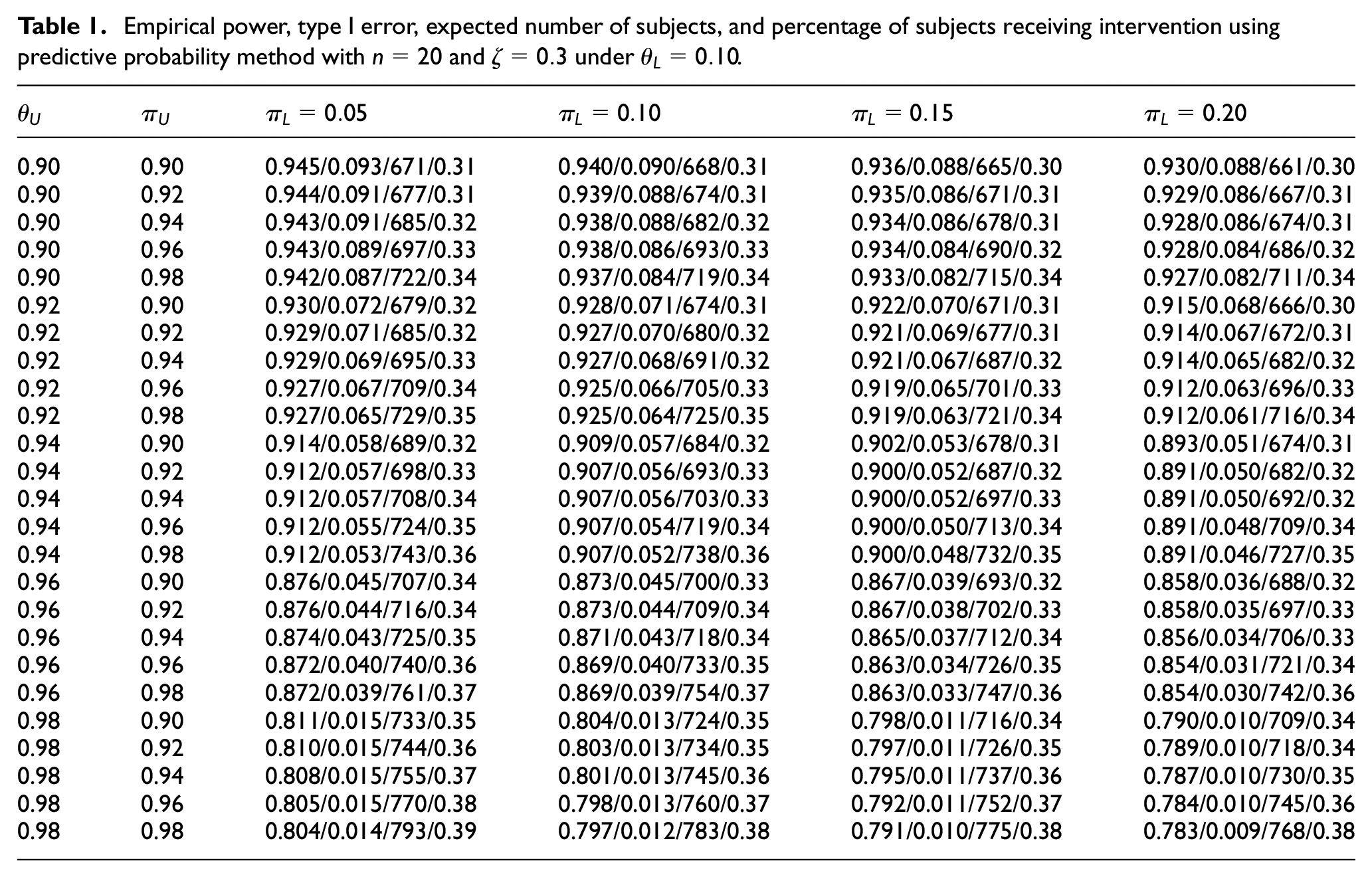
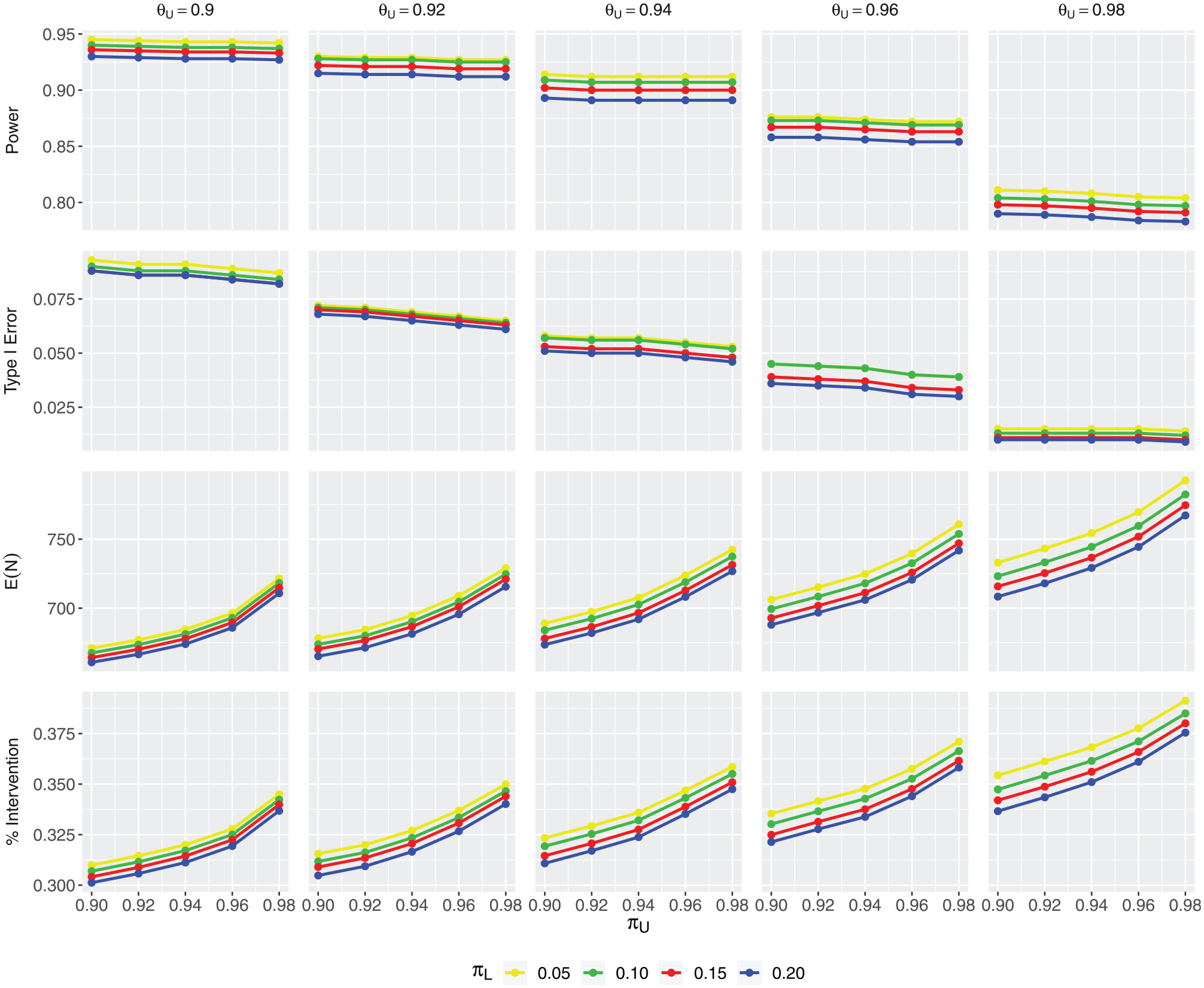
We first assess the impact of various decision thresholds $({\theta }_U,{\pi }_U,{\pi }_L,{\theta }_L)$ on operating characteristics, including power, type I error, expected sample size (denoted by $E(N)$ ), and the percentage of patients receiving intervention (denoted by intervention%). Table 1 presents the simulation results based on Algorithm 1, given $n=20$ , $\zeta =0.3$ , and ${\theta }_L=0.1$ . First note that with $n=20$ , $J=10$ , and $T=5$ , the sample size in a complete SW-CRT is 1000. Under the Bayesian adaptive design, due to the possibility of early stopping, $E(N)$ ranges from 793 to 661. Also, intervention% = 0.5 in a complete trial. Because all clusters start from control, early stopping would always result in intervention% < 0.5. In Table 1, we observe a range of 0.31–0.39 in intervention%. A larger probability of early stopping is generally associated with a smaller $E(N)$ and intervention%. Along each row, with all the other thresholds fixed, as ${\pi }_L$ increases, we observe simultaneous decrease in empirical power, type I error, $E(N)$ , and intervention%. A larger ${\pi }_L$ makes it easier to stop early for futility, which leads to a decreased $E(N)$ and intervention%. Furthermore, a greater probability of stopping early for futility tends to reduce the chance of crossing the efficacy threshold, hence decreased power and type I error. However, along the columns, as ${\pi }_U$ increases, we observe decreasing power and type I error, but increasing $E(N)$ and intervention%. The reason is that a larger ${\pi }_U$ makes it harder to stop early for efficacy, hence reduced power and type I error. A smaller probability of early stopping also leads to larger $E(N)$ and intervention%. The impact of ${\theta }_U$ is in the same direction as ${\pi }_U$ , but more pronounced. For example, under $({\theta }_U=0.9,{\pi }_U=0.9,{\pi }_L=0.05,{\theta }_L=0.1)$ , the (power, type I error, $E(N)$ , intervention%) are (0.945, 0.093, 671, 0.31). When ${\pi }_U$ increases from 0.9 to 0.92, the operating characteristics only change slightly to (0.944, 0.091, 677, 0.31). However, when ${\theta }_U$ increases from 0.9 to 0.92, the operating characteristics change more dramatically to (0.93, 0.072, 679, 0.32). The reason is that ${\theta }_U$ is involved both in interim decisions (through $P{P}_t$ ) and the decision at the end of study. Finally, the effect of ${\theta }_L$ is minimal because it only affects the study when the study doesn’t stop early and continues to the last step. The results under ${\theta }_L=(0.05,0.15,0.20)$ are the same as those presented in Table 1 on rounding to the fourth digit after the decimal point. To better illustrate the impact of decision thresholds on trial properties, we have constructed a series of plots corresponding to Table 1. Figure 1 contains $4\times 5$ panels. The four rows show empirical power, type I error, $E(N)$ , and intervention%, respectively. The five columns correspond to different values of ${\theta }_U$ explored. Within each panel, the horizontal axis shows values of ${\pi }_U$ and the color of each curve indicates the value of ${\pi }_L$ . Due to page limit, the plots for $n=15$ and $n=25$ are presented in the Supplemental Material.

Table 1.

Empirical power, type I error, expected number of subjects, and percentage of subjects receiving intervention using predictive probability method with $n=20$ and $\zeta =0.3$ under ${\theta }_L=0.10$ .

${\theta }_U$	${\pi }_U$	${\pi }_L=0.05$	${\pi }_L=0.10$	${\pi }_L=0.15$	${\pi }_L=0.20$
0.90	0.90	0.945/0.093/671/0.31	0.940/0.090/668/0.31	0.936/0.088/665/0.30	0.930/0.088/661/0.30
0.90	0.92	0.944/0.091/677/0.31	0.939/0.088/674/0.31	0.935/0.086/671/0.31	0.929/0.086/667/0.31
0.90	0.94	0.943/0.091/685/0.32	0.938/0.088/682/0.32	0.934/0.086/678/0.31	0.928/0.086/674/0.31
0.90	0.96	0.943/0.089/697/0.33	0.938/0.086/693/0.33	0.934/0.084/690/0.32	0.928/0.084/686/0.32
0.90	0.98	0.942/0.087/722/0.34	0.937/0.084/719/0.34	0.933/0.082/715/0.34	0.927/0.082/711/0.34
0.92	0.90	0.930/0.072/679/0.32	0.928/0.071/674/0.31	0.922/0.070/671/0.31	0.915/0.068/666/0.30
0.92	0.92	0.929/0.071/685/0.32	0.927/0.070/680/0.32	0.921/0.069/677/0.31	0.914/0.067/672/0.31
0.92	0.94	0.929/0.069/695/0.33	0.927/0.068/691/0.32	0.921/0.067/687/0.32	0.914/0.065/682/0.32
0.92	0.96	0.927/0.067/709/0.34	0.925/0.066/705/0.33	0.919/0.065/701/0.33	0.912/0.063/696/0.33
0.92	0.98	0.927/0.065/729/0.35	0.925/0.064/725/0.35	0.919/0.063/721/0.34	0.912/0.061/716/0.34
0.94	0.90	0.914/0.058/689/0.32	0.909/0.057/684/0.32	0.902/0.053/678/0.31	0.893/0.051/674/0.31
0.94	0.92	0.912/0.057/698/0.33	0.907/0.056/693/0.33	0.900/0.052/687/0.32	0.891/0.050/682/0.32
0.94	0.94	0.912/0.057/708/0.34	0.907/0.056/703/0.33	0.900/0.052/697/0.33	0.891/0.050/692/0.32
0.94	0.96	0.912/0.055/724/0.35	0.907/0.054/719/0.34	0.900/0.050/713/0.34	0.891/0.048/709/0.34
0.94	0.98	0.912/0.053/743/0.36	0.907/0.052/738/0.36	0.900/0.048/732/0.35	0.891/0.046/727/0.35
0.96	0.90	0.876/0.045/707/0.34	0.873/0.045/700/0.33	0.867/0.039/693/0.32	0.858/0.036/688/0.32
0.96	0.92	0.876/0.044/716/0.34	0.873/0.044/709/0.34	0.867/0.038/702/0.33	0.858/0.035/697/0.33
0.96	0.94	0.874/0.043/725/0.35	0.871/0.043/718/0.34	0.865/0.037/712/0.34	0.856/0.034/706/0.33
0.96	0.96	0.872/0.040/740/0.36	0.869/0.040/733/0.35	0.863/0.034/726/0.35	0.854/0.031/721/0.34
0.96	0.98	0.872/0.039/761/0.37	0.869/0.039/754/0.37	0.863/0.033/747/0.36	0.854/0.030/742/0.36
0.98	0.90	0.811/0.015/733/0.35	0.804/0.013/724/0.35	0.798/0.011/716/0.34	0.790/0.010/709/0.34
0.98	0.92	0.810/0.015/744/0.36	0.803/0.013/734/0.35	0.797/0.011/726/0.35	0.789/0.010/718/0.34
0.98	0.94	0.808/0.015/755/0.37	0.801/0.013/745/0.36	0.795/0.011/737/0.36	0.787/0.010/730/0.35
0.98	0.96	0.805/0.015/770/0.38	0.798/0.013/760/0.37	0.792/0.011/752/0.37	0.784/0.010/745/0.36
0.98	0.98	0.804/0.014/793/0.39	0.797/0.012/783/0.38	0.791/0.010/775/0.38	0.783/0.009/768/0.38

Figure 1.

The plot of operating characteristics under $n=20$ and ${\theta }_L=0.10$ . The four rows show empirical power, type I error, $E(N)$ , and intervention%, respectively. The five columns correspond to different values of ${\theta }_U$ . Within each panel, the horizontal axis shows values of ${\pi }_U$ and the color of each curve corresponds to a different value of ${\pi }_L$ .

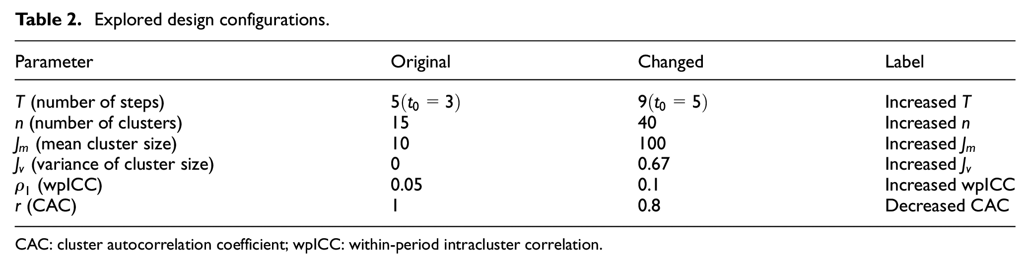
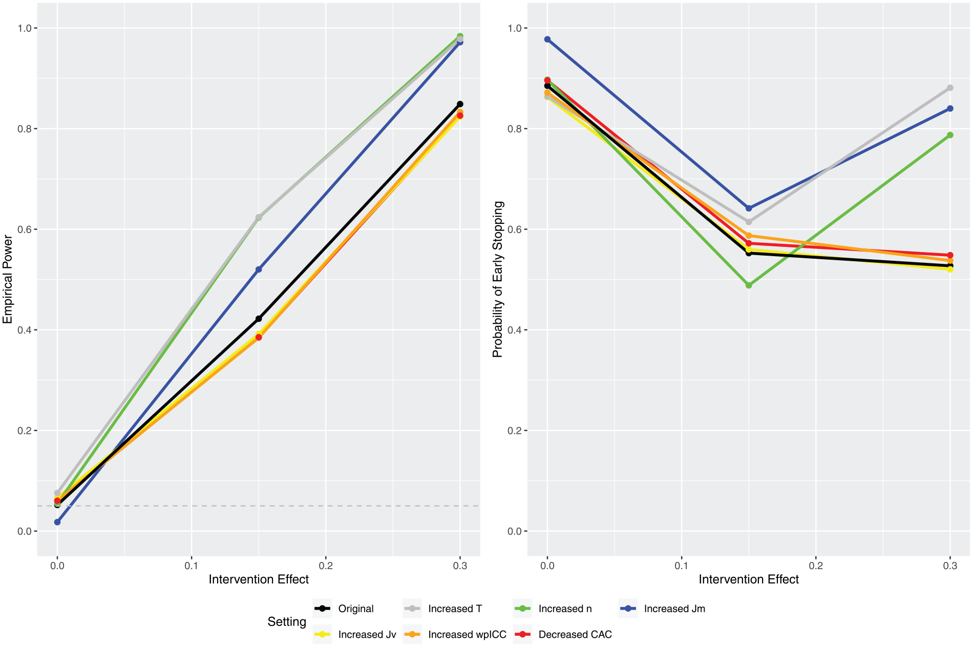
To evaluate the impact of various design factors, we start from an “Original” configuration, and one-by-one change each of the design parameters to assess its marginal effect on trial properties. In Table 2, the second column contains the parameter values under “Original.” Note that $J_v=0$ indicates a constant cluster size, and $r=1$ indicates an exchangeable correlation structure. The third column contains the changed value of each parameter, with the corresponding label listed in the last column. For example, under “Increased n,” the number of clusters is changed from 15 to 40, while all other parameters remain unchanged. For “Increased $J_v$ ,” we assume that cluster sizes $\left(J_{\mathit{it}}\right)$ follow a discrete uniform distribution between 8 and 12, denoted by DU[8,12]. It centers around mean $J_m=10$ with variance $J_v=0.67$ . Hence, comparing “Increased $J_v$ ” versus “Original” allows us to assess the impact of random variability in cluster size. For “Decreased CAC,” $r$ changes from 1 to 0.8, which leads to a block exchangeable correlation structure, with a bpICC ${\rho }_2=0.04$ . Under the block exchangeable correlation structure, $r$ is a model parameter with a Beta(5,2) prior, which has a mode of 0.8.

Table 2.

Explored design configurations.

Parameter	Original	Changed	Label
$T$ (number of steps)	$5(t_0=3)$	$9(t_0=5)$	Increased $T$
$n$ (number of clusters)	15	40	Increased $n$
$J_m$ (mean cluster size)	10	100	Increased $J_m$
$J_v$ (variance of cluster size)	0	0.67	Increased $J_v$
${\rho }_1$ (wpICC)	0.05	0.1	Increased wpICC
$r$ (CAC)	1	0.8	Decreased CAC

CAC: cluster autocorrelation coefficient; wpICC: within-period intracluster correlation.

In Figure 2, the left panel presents the empirical powers under different configurations where the true values of intervention effect are set at $\zeta =0,0.15$ , and 0.3. The right panel shows the corresponding probabilities of early stopping. The power at $\zeta =0$ is the type I error. The threshold values $({\theta }_U,{\pi }_U,{\pi }_L,{\theta }_L)$ are selected under “Original” to achieve power and type I error around 0.85 and 0.05, respectively, at $\zeta =0.3$ . To examine the change in operational characteristics without confounding by thresholds, the same threshold values are used across all configurations. As a result, the type I errors obtained under configurations other than “Original” do not necessarily fall at 0.05. If the results show much greater increase in power than in type I error, however, we can generally conclude a net gain in power. We observe significant increase in power under an increased number of steps $\left(T\right)$ , an increased number of clusters $\left(n\right)$ , and an increased cluster size $\left(J_m\right)$ . However, the additional variability in cluster size (increased $J_v$ ) leads to reduced power. Finally, increasing the correlation under an exchangeable correlation structure (“increased wpICC”) and changing the correlation structure from exchangeable $(\mathit{CAC}=1)$ to block exchangeable $(\mathit{CAC}=0.8)$ both lead to decreased power. These observations are consistent with the findings by Matthews and Forbes ³⁰ and Hooper et al., ²⁶ who reported that the relationship between wpICC or CAC and the variance of estimated treatment effect generally follows a ∩ shape, increasing from 0 and decreasing approaching 1. When wpICC increases from 0.05 to 0.1, it follows the initial ascending trend, which leads to an increased variance of estimated treatment effect and a decreased power. However, when CAC decreases from 1 to 0.8, it traces back the descending trend around 1, which also leads to an increased variance and a decreased power.

Figure 2.

The marginal impact of various design parameters.

In the right panel of Figure 2, the impact of design parameters on the probability of early stopping is less straightforward. Our experience has been that the thresholds’ impact on power (especially when considering net gain described above) is relatively smaller compared with their impact on the probability of early stopping because the interim thresholds ${\pi }_U$ and ${\pi }_L$ directly affect early stopping decisions. Hence, we caution against over-interpreting the right panel because the thresholds are selected to achieve certain characteristics under “Original,” which have no bearing on the other configurations. Nonetheless, we have a few useful observations. First note that the probability of early stopping usually follows a $U-\mathrm{shape}$ . To explain, define $g_F$ and $g_E$ to be the probability of early stopping due to futility and efficacy, respectively. When the true intervention effect is small, the probability of early stopping is large due to large $g_F$ ; as the intervention effect increases, $g_F$ decreases faster than $g_E$ increases, and the overall probability of early stopping continues to decrease; when the intervention effect is sufficiently large, $g_E$ begins to increase faster than $g_F$ decreases, and the overall probability of early stopping passes the bottom of the $U-\mathrm{shape}$ and begins to increase continuously. We observe that under larger cluster sizes (“Increased $J_m$ ”), more steps (“Increased $T$ ”), and more clusters (“Increased $n$ ”), the overall probabilities of early stopping all follow the typic $U-\mathrm{shape}$ because these configurations significantly increase power, resulting in the extreme intervention effect $(\zeta =0.3)$ being well above the bottom of the $U-\mathrm{shape}$ . However, we observe that under “Original,” the probability of early stopping remains on the left-hand side of the $U-\mathrm{shape}$ due to its relatively smaller power. Finally, we observe that variability in cluster size (“Increases $J_v$ ”), stronger correlation (“Increased wpICC”), and changing to a block exchangeable correlation structure (“Decreased CAC”), have relatively smaller effect on the probability of early stopping.

Finally, we investigate the impact of informative priors. We conduct simulation using the same design configuration as that of the “Original” in Figure 2, except that the prior of treatment effect $\zeta$ is changed to $N(0.15,1)$ and $N(0.3,1)$ . Recall that a non-informative prior is assumed for $\zeta$ under the “Original.” Given true intervention effect $\zeta =0.3$ , the prior $N(0.3,1)$ centers around the true effect with variance 1, while $N(0.15,1)$ represents a mis-specified prior. The (power, type I error) under the “Original,” $N(0.15,1)$ , and $N(0.3,1)$ are (0.849, 0.052), (0.851, 0.063), and (0.862, 0.07), respectively. We observe a trend of slight increase both in power and type I error. This is to be expected because compared with the non-informative prior, both $N(0.15,1)$ and $N(0.3,1)$ shift the posterior distribution of $\zeta$ toward the direction of true intervention effect, increasing the probability of rejecting the null hypothesis, hence increased power and type I error. Overall, the gain in power using an informative prior is pretty much canceled by increased type I error. In Bayesian Phase I or Phase II trials because the sample sizes are usually small, informative priors can have greater impact on trial properties. For Phase III or SW trials, where the sample sizes are usually large, the impact of informative priors is less obvious.

An application example

We illustrate the proposed Bayesian adaptive method using a pragmatic cross-sectional SW-CRT, which evaluates the effect of a combined intervention on preventing malnutrition and reducing weight loss in hospitalized patients with acute tertiary care. ³¹ The evidence-based intervention consists of three linked activities: the introduction and use of the Malnutrition Universal Screening Tool (MUST), the provision of food supplements to patients at risk of malnutrition, and a system that uses red feeding trays to flag patients requiring full feeding assistance. Two trained local facilitators (a nurse and dietitian for each group) will introduce the intervention. The control arm receives the standard care. There are $T=5$ steps and the randomization unit is ward, each with $J=20$ patients. The wards are randomized to $S=4$ sequences. The primary outcome is the rate of change in patient’s body mass index. We assume an exchangeable correlation structure with ${\rho }_1=0.03$ . The assumed target intervention effect is $\zeta =0.3$ . The adaptation starts from step $t_0=3$ . A recent implementation project on nutrition screening and documentation found substantial improvement in hospital wards and identified widespread interest in further improvement to nutritional status and care of vulnerable patients.^32,33 A number of internal, unpublished audits have identified that up to half of patients are at risk of nutritional decline in systems that do not prioritize patient nutrition. Hence, implementing the Bayesian group sequential strategy makes it possible for the SW-CRT to stop early, hastening the adoption of effective interventions in the patient population with high prevalence of risk. The goal is to determine the design configuration, including n (the number of wards) and decision thresholds $({\theta }_U,{\theta }_L,{\pi }_U,{\pi }_L)$ , that achieves desired trial properties.

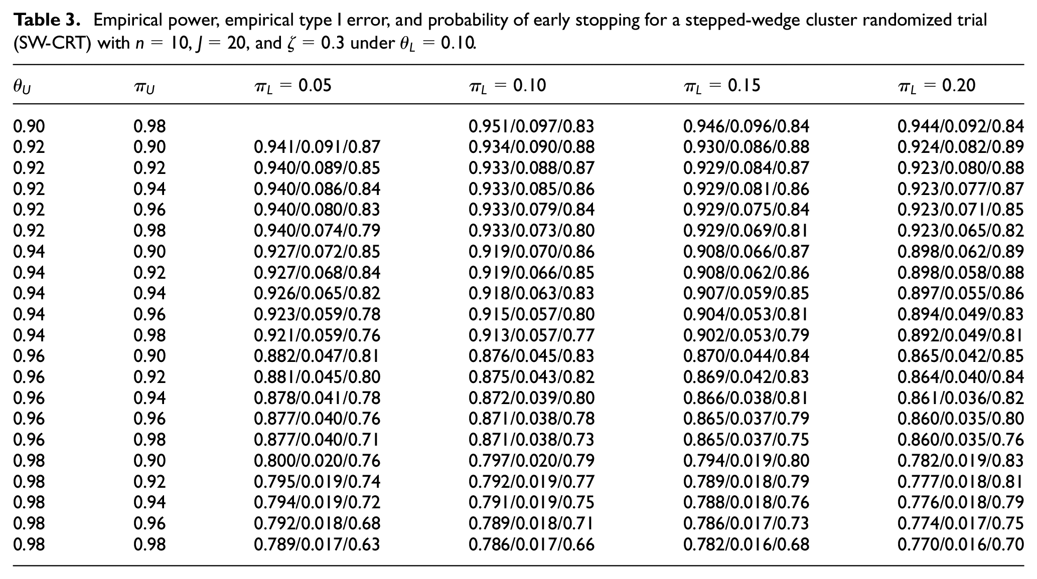
For each n, a range of thresholds values: $\{0.90,0.92,0.94,0.96,0.98\}$ for ${\theta }_U$ and ${\pi }_U$ ; and $\{0.05,0.10,0.15,0.20\}$ for ${\pi }_L$ are explored. Because simulation studies suggest that ${\theta }_L$ has minimal effect on trial properties, we fix it at ${\theta }_L=0.10$ . For illustration purpose, Table 3 presents results under $n=10$ wards, where each cell shows empirical power, type I error, and the probability of early stopping given a combination of threshold values. Cells with empirical type I errors greater than 0.1 are considered unacceptable and omitted. The table is divided into four areas. From top to bottom:

Table 3.

Empirical power, empirical type I error, and probability of early stopping for a stepped-wedge cluster randomized trial (SW-CRT) with $n=10$ , $J=20$ , and $\zeta =0.3$ under ${\theta }_L=0.10$ .

${\theta }_U$	${\pi }_U$	${\pi }_L=0.05$	${\pi }_L=0.10$	${\pi }_L=0.15$	${\pi }_L=0.20$
0.90	0.98		0.951/0.097/0.83	0.946/0.096/0.84	0.944/0.092/0.84
0.92	0.90	0.941/0.091/0.87	0.934/0.090/0.88	0.930/0.086/0.88	0.924/0.082/0.89
0.92	0.92	0.940/0.089/0.85	0.933/0.088/0.87	0.929/0.084/0.87	0.923/0.080/0.88
0.92	0.94	0.940/0.086/0.84	0.933/0.085/0.86	0.929/0.081/0.86	0.923/0.077/0.87
0.92	0.96	0.940/0.080/0.83	0.933/0.079/0.84	0.929/0.075/0.84	0.923/0.071/0.85
0.92	0.98	0.940/0.074/0.79	0.933/0.073/0.80	0.929/0.069/0.81	0.923/0.065/0.82
0.94	0.90	0.927/0.072/0.85	0.919/0.070/0.86	0.908/0.066/0.87	0.898/0.062/0.89
0.94	0.92	0.927/0.068/0.84	0.919/0.066/0.85	0.908/0.062/0.86	0.898/0.058/0.88
0.94	0.94	0.926/0.065/0.82	0.918/0.063/0.83	0.907/0.059/0.85	0.897/0.055/0.86
0.94	0.96	0.923/0.059/0.78	0.915/0.057/0.80	0.904/0.053/0.81	0.894/0.049/0.83
0.94	0.98	0.921/0.059/0.76	0.913/0.057/0.77	0.902/0.053/0.79	0.892/0.049/0.81
0.96	0.90	0.882/0.047/0.81	0.876/0.045/0.83	0.870/0.044/0.84	0.865/0.042/0.85
0.96	0.92	0.881/0.045/0.80	0.875/0.043/0.82	0.869/0.042/0.83	0.864/0.040/0.84
0.96	0.94	0.878/0.041/0.78	0.872/0.039/0.80	0.866/0.038/0.81	0.861/0.036/0.82
0.96	0.96	0.877/0.040/0.76	0.871/0.038/0.78	0.865/0.037/0.79	0.860/0.035/0.80
0.96	0.98	0.877/0.040/0.71	0.871/0.038/0.73	0.865/0.037/0.75	0.860/0.035/0.76
0.98	0.90	0.800/0.020/0.76	0.797/0.020/0.79	0.794/0.019/0.80	0.782/0.019/0.83
0.98	0.92	0.795/0.019/0.74	0.792/0.019/0.77	0.789/0.018/0.79	0.777/0.018/0.81
0.98	0.94	0.794/0.019/0.72	0.791/0.019/0.75	0.788/0.018/0.76	0.776/0.018/0.79
0.98	0.96	0.792/0.018/0.68	0.789/0.018/0.71	0.786/0.017/0.73	0.774/0.017/0.75
0.98	0.98	0.789/0.017/0.63	0.786/0.017/0.66	0.782/0.016/0.68	0.770/0.016/0.70

• Area 1: $0.90\le$  Empirical power and 0.05 ≤ Empirical type I error < 0.10;

• Area 2: $0.80\le$  Empirical power < 0.90 and 0.05 ≤ Empirical type I error < 0.10;

• Area 3: $0.80\le$  Empirical power < 0.90 and Empirical type I error < 0.05;

• Area 4: $0.70\le$  Empirical power < 0.80 and Empirical type I error < 0.05.

If researchers would like to achieve power $\ge 0.9$ and type I error $\le 0.1$ , then we can search within Area 1, and thresholds $({\theta }_U,{\theta }_L,{\pi }_U,{\pi }_L)=(0.92,0.10,0.90,0.20)$ might be chosen, based on the consideration that it maximizes the probability of early stopping (0.89). However, if the goal is to achieve power $\ge 0.8$ and type I error $\le 0.05$ , then $({\theta }_U,{\theta }_L,{\pi }_U,{\pi }_L)=(0.94,0.10,0.98,0.20)$ might be selected to achieve the maximum power (0.894). We cannot find thresholds that achieve power $\ge 0.9$ and type I error $\le 0.05$ . It means that adjustment of threshold values is insufficient, and a larger number of clusters $\left(n\right)$ is needed to achieve the higher level of power.

Conclusion

In this study we proposed to incorporate Bayesian adaptive strategies into SW-CRTs, where adaptive decisions are made based on the predictive probability of declaring the intervention effective at the end of study given interim observations. The proposed method offers flexibility to stop the trial early if overwhelming evidence of effectiveness or futility is observed at interim. Compared with frequentist design methods for SW-CRTs, the proposed Bayesian method requires additional specification of decision thresholds $({\theta }_U,{\theta }_L,{\pi }_U,{\pi }_L)$ . Design parameters are determined through numerical studies to achieve desired operating characteristics. We conducted extensive simulation studies to examine the performance of the Bayesian SW-CRTs over different design configurations. We presented the Bayesian adaptive method based on a cross-sectional SW-CRT. By modifying the likelihood function, this method can also be applied to closed-cohort SW-CRTs where the same cohort of subjects is followed through the whole study period.

Incorporating Bayesian adaptive strategies into SW-CRTs can offer notable gains in terms of saving time and resources, and in improved ethics. However, several practical considerations are needed. Bayesian adaptive strategies generally require additional resources to conduct extensive simulation studies in trial design, and timely data collection, processing, and analysis to support adaptive decisions at interim. Although the crossover scheme of SW-CRTs lends themselves well to the Bayesian adaptive strategies, it has a strict requirement on time frame. The intervention is assumed to show measurable effect within the duration of a step. The proposed adaptive design is feasible when there is enough time between steps to allow measuring outcomes and conducting interim analysis.^34–36 In this study, we assume a constant intervention effect, which effectively assumes no apparent learning-curve effect in the implementation of intervention.

A potential extension is to introduce a mechanism that adaptively adjusts assignment probabilities based on interim results. For example, if interim analysis suggests that the intervention is promising, this mechanism allows researchers to probabilistically hasten the transition of remaining clusters (under control) to intervention. Such an adaptive strategy has been shown to increase the number of patients receiving a more effective intervention and improve patient outcomes. ³⁷ Grayling et al. ³⁸ proposed a frequentist response adaptive approach that permits modification of the intervention allocation during an SW-CRT. Incorporating a Bayesian response adaptive strategy into SW-CRTs to adjust assignment probabilities will be the topic of our future research.

Supplemental Material

sj-7z-2-ctj-10.1177_17407745231221438 – Supplemental material for A Bayesian adaptive design approach for stepped-wedge cluster randomized trials

Supplemental material, sj-7z-2-ctj-10.1177_17407745231221438 for A Bayesian adaptive design approach for stepped-wedge cluster randomized trials by Jijia Wang, Jing Cao, Chul Ahn and Song Zhang in Clinical Trials

Supplemental Material

sj-pdf-1-ctj-10.1177_17407745231221438 – Supplemental material for A Bayesian adaptive design approach for stepped-wedge cluster randomized trials

Supplemental material, sj-pdf-1-ctj-10.1177_17407745231221438 for A Bayesian adaptive design approach for stepped-wedge cluster randomized trials by Jijia Wang, Jing Cao, Chul Ahn and Song Zhang in Clinical Trials