
Abstract
In this article, a systematic procedure is given for determining a robust motion control law for autonomous quadcopters, starting from an input–output linearizable model. In particular, the suggested technique can be considered as a robust feedback linearization (FL), where the nonlinear state-feedback terms, which contain the aerodynamic forces and moments and other unknown disturbances, are estimated online by means of extended state observers. Therefore, the control system is made robust against unmodelled dynamics and endogenous as well as exogenous disturbances. The desired closed-loop dynamics is obtained by means of pole assignment. To have a feasible control action, that is, the forces produced by the motors belong to an admissible set of forces, suitable reference signals are generated by means of differentiators supplied by the desired trajectory. The proposed control algorithm is tested by means of simulation experiments on a Raspberry-PI board by means of the hardware-in-the-loop method, showing the effectiveness of the proposed approach. Moreover, it is compared with the standard FL control method, where the above nonlinear terms are computed using nominal parameters and the aerodynamical disturbances are neglected. The comparison shows that the control algorithm based on the online estimation of the above nonlinear state-feedback terms gives better static and dynamic behaviour over the standard FL control method.
Keywords
Introduction
In the last years, the control of unmanned mobile vehicles has received great attention. This interest is motivated by many applications, where the autonomous control is required, such as the tracking of a trajectory for the accomplishment of a particular task. On this subject, a huge number of works propose valid control solutions, especially in the field of aerial vehicles. Most of these solutions have been summarized in several articles and books (see, for example, the lierature 1,2,3,4 and references therein).
In this work, the attention is focused on the control of autonomous quadcopter vehicles. With regard to this field, many problems have been addressed in the literature. The feedback linearization (FL) via dynamic feedback has been shown in the literature,
5
starting from the classical mathematical model of the vehicle with 12 state variables, which is not input–output linearizable. From this model, using the method of the input dynamic feedback and neglecting the exogenous disturbances, a model with 14 state variables is obtained, which results in input–output linearizable. The model linearized by means of FL appears decoupled in four SISO models having the three components of the position vector referred to as an inertial reference frame and the yaw angle as outputs, and an auxiliary input vector with four components. A state-feedback controller is then designed for each of the above four models using the pole assignment technique. Simulation results confirm the feasibility of the controller based on the linearized and decoupled model. In the literature,
6
the input–output linearized and decoupled model is completed by adding to the auxiliary input and the vector of the four exogenous equivalent disturbances projected on this input space. In this way, four linear decoupled and time-invariant models are obtained, each of them differs from the Brunovsky canonical form for the presence of an unknown equivalent disturbance added to a component of the auxiliary input vector. The four components of the equivalent disturbance vector are computed from the state variables estimated by means of a high-order sliding-mode state observer, and then, they are conveniently filtered by means of a filter not indicated in the article, and the filtered values are used to compensate for exogenous disturbances. Consequently, the determination of these components is open-loop type. The remaining attitude variables and the angular velocities in BODY frame, not estimated by the sliding observer, are computed using the estimated variables and the above mentioned linearizable model without exogenous disturbances. The last variables and those estimated are used for the implementation of the control law. In the literature,
7
PID-type classical control techniques and optimal linear quadratic control are employed using linear approximated models only for attitude control. An adaptive version of optimal controller is also discussed. In the literature,
8
Taamallah et al. deal with the online planning of a trajectory for a helicopter with an engine OFF flight condition and robust tracking of the planned trajectory. The planning approach is model-based and feasible and optimal trajectories can be generated. Regarding the controller design, the
This article deals with the motion control of autonomous quadcopters, which can track a desired trajectory ensuring a high dynamic performance and the robustness of the whole system. The robust motion control is designed so as to satisfy the following requirements: (a) decoupling of the linear motions along the three axes of the inertial frame and the yaw angle; (b) robustness against endogenous and exogenous disturbances; (c) assignment of the desired dynamics to each of the above decoupled motions and (d) the control actions, i.e., the forces to be produced by the motors, have to belong to the admissible set of forces, i.e., the set of forces that the motor propeller is able to generate. To satisfy the above requirements, a combination of FL and active disturbance rejection approaches is utilized. More precisely, starting from the 14-order nonlinear model illustrated in the literature,
6
defining a convenient nonlinear equivalent disturbance vector which contains both the endogenous disturbances and the exogenous ones, assuming known equivalent disturbance, a linear model is obtained consisting of four linear and decoupled models, each of them having the Brunovsky canonical form, forced only by means of a component of the auxiliary input. This goal has been achieved by applying the nonlinear control theory shown in the literature.
12,13
Different from the procedure used in the litreature,
6
each component of the nonlinear equivalent disturbance vector is online estimated by means of an extended state observer (ESO) and this guarantees robustness of the proposed control law. In this way, the requirements of (a) and (b) are satisfied. Note that the applied technique is also different from the
The validation of the control law is carried out by means of several simulations and the standard mathematical model of the quadrotor. To increase accuracy of the simulations, the controller has been discretized and it has been executed with a fixed sampling time in a Raspberry-PI board by means of the hardware-in-the-loop method. Moreover, the quantization level of the measured signals has been taken into consideration, as well as the fact that the data acquired by the IMU and the GPS, i.e., position and velocity of the quadrotor center of mass, are available with different rates is also considered. This is bargained for using the hybrid nonlinear observer illustrated in the literature. 14 Besides this, the robustness of the designed control law is another aspect, which increases the effectiveness of the controller and the feasibility of its experimental implementation. To the best of the authors’ knowledge, the control architecture proposed in this work, for quadcopter control, is not described in the literature.
List of symbols.

Preliminaries on the mathematical model of the quadcopter
The mathematical model of the quadcopter considered in this article is the state-space model obtained in the literature
1
and considered also in the literature.
5,6
The state variables are the coordinates of the center of gravity (x, y and z) of the vehicle referred to an inertial frame NED, the speeds (u, v and w) referred to the same frame, the Euler angles (roll
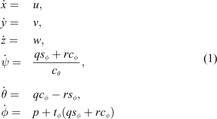
Cinematic model
Dynamical model
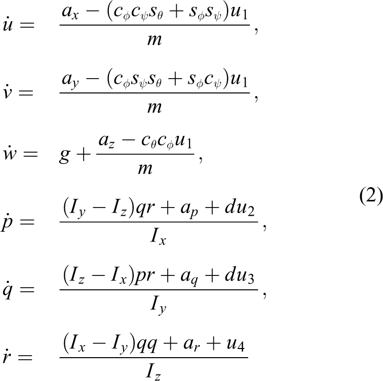
The symbols are defined in Table 1. Models (1) and (2) have four input variables, denoted by ui
,

The above equations allow to obtain the forces fi
starting from the inputs ui
. Since for assigned ui
,

Scheme of the quadcopter.
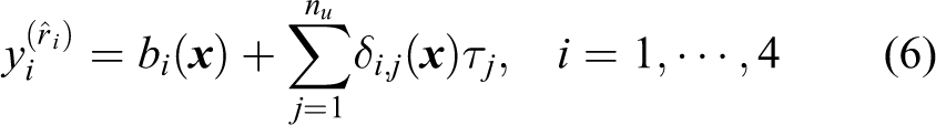
Finally, the output is given by

Assumption 1. To avoid singularity problems, the following constraint is assumed for models (1) and (2)

Note that this constraint is satisfied in a correct operation of a quadcopter vehicle, and unlikely, the quadcopter reaches the boundary of this domain, where singularity problems can occur (
In the literature,
5
it is shown that the models (1) and (2) have a vector relative degree equal to

The vector relative degree of models (1) and (5) is given by
where

These equations, in matrix form, can be written as follows

where


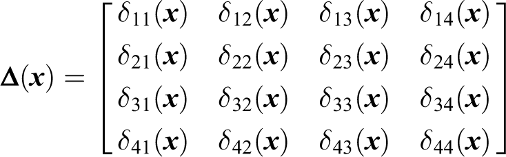
The terms
The determinant of matrix
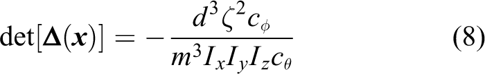
It follows that, under Assumption 1,
Design of the control algorithm
Now, the motion control law for model (7) has to be designed so as to satisfy the following requirements: decoupling of the motions along the three axes of the inertial frame and that of the orientation along the yaw angle; robustness against endogenous and exogenous disturbances; each of the above decoupled motions has to occur according to the given dynamics; the control actions, i.e., the forces to be produced by the motor propellers, belong to the set of forces that the propellers can generate.
As it will be seen later, items (a) and (b) are obtained if good knowledge is gained on the disturbance vector and on the control gain matrix. Item (c) will be satisfied using pole assignment techniques. Item (d) will be gained by choosing suitably the dynamics of the whole closed-loop control system.
Control architecture
The structure of equation (7) is such that if the control gain matrix,

where

It is worthwhile to observe that model (10) consists of four chains of integrators of orders
However, to apply the control law (9), a good knowledge of
Motivated from these considerations, it proposed a control law based on the disturbance vector estimation,

If the estimation of the disturbance vector is sufficiently accurate (i.e.
The control law previously described appears, practically, as a FL control in which the nonlinear term, representing endogenous and exogenous disturbances, is online estimated instead of analytically computed. This technique is called active disturbance rejection control (ADRC)
15
The nonlinear disturbance
Design of the extended state observers
In the present article, we will obtain the estimation of the disturbance vector by constructing four ESOs designed from model (7).
In particular, this model can be divided into four independent submodels as follows

With reference to model (12), let us define the following extended state vector

Then, it is possible to define the following extended state model

An ESO for model (14) has the following structure (16)
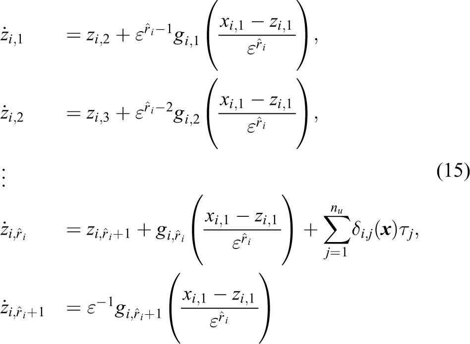
for
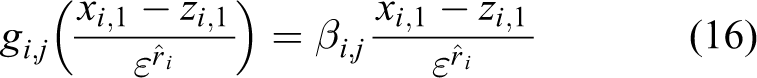
where
Defining, now, the following error variables

and by taking into account equations (15) and (16), the following error dynamics are obtained

Equation (18) can be expressed in matrix form as follows

where

In the literature,
16
it is shown that for a given
Design of the controller
With reference to the design of the controller, the starting point is the knowledge of a good estimate of the disturbance vector. Then, it is possible to apply the control law (11) to model (7), thus obtaining model (10).
This model can be divided into four submodels as follows

The state-space models associated with equation (20) are
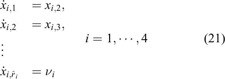
which is the Brunovsky canonical form. For this model, the control law is obtained so as to assign the desired dynamics to the corresponding closed-loop system. Note that this fact is important because it shows that it is possible to obtain four independent submodels, and these submodels can be controlled by four independent inputs
By denoting with
leads to

where

are Hurwitz, then
Differentiators design
This section deals with linear and nonlinear differentiators (LD and ND, respectively). These dynamical systems, starting from the desired motion in the output space
According to the literature, 17 the structure of an ND of order n is given by

where

and the coefficients

is Hurwitz. Model (25) allows to estimate the derivatives of yd
up to that of order
Equation (26) shows that

with

Model (28) is asymptotically stable, and its transfer function, from

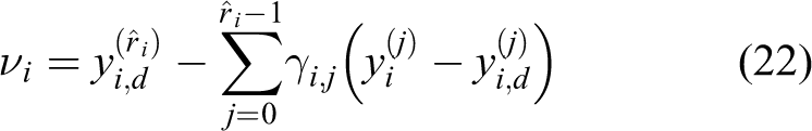
The tracking error

It follows that the LD tracks constantly desired signals with null steady-state error and ramp desired signals with a steady-state error equal to
Testing of the control law
To test the control laws designed in the previous sections, simulations have been carried out by means of hardware-in-the-loop method. In particular, the control law has been implemented in a Raspberry-PI with a sampling frequency of 100 Hz as well as the reference trajectories and the hybrid nonlinear observer described below to perform the data fusion between GPS, working at 10 Hz, and IMU, whose measurements occur at the same frequency of the controller. The quadcopter has been simulated in MATLAB-Simulink environments, implementing equations (1) to (3) and considering the following parameters 18
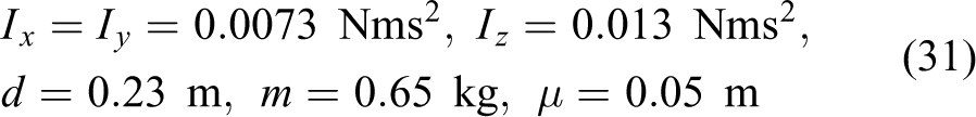
The aerodynamic forces are chosen as

x, y and z reference components of the quadrotor during the simulation experiment.

Reference yaw angle of the quadrotor during the simulation experiment.
The ESOs for the positioning that estimate the equivalent disturbances along the axes x, y and z have been designed so that the eigenvalues of the corresponding dynamical matrix

With reference to the ESO for the orientation

With reference to the controllers for positioning and orientation (yaw), they have been designed by means of the pole assignment technique so that the polynomial (24) is equal to
The differentiators are designed to constraint the forces generated by the four propellers to the interval

while, for orientation, an ND has been considered such that

Data fusion of IMU and GPS measurements
In this subsection, the problem of data fusion between measurements given by IMU (sampled at 100 Hz) and measurements given by GPS (sampled at 10 Hz) is discussed. Since the measurement systems used in this field have a low update rate with respect to the control algorithm, a suitable observer with sampled measurements has to be designed. Moreover, also, the fact that the time between two consecutive measurements is not constant, but it can vary randomly, has to be considered. For these reasons, the data fusion process between data given by the above-mentioned devices is governed by the hybrid nonlinear observer described in the literature, 14 based on the strap-down model of the IMU. In particular, the observer combines a nonlinear Luenberger-type observer (NLTO), which gives the state estimate, and a updating mechanism, which carries out a corrective action on the NLTO when new position and velocity vector measurements arrive from GPS. The NLTO is realized so that its update avoids discontinuities in the estimate. For further details, the reader is addressed to the literature. 14
Simulation results
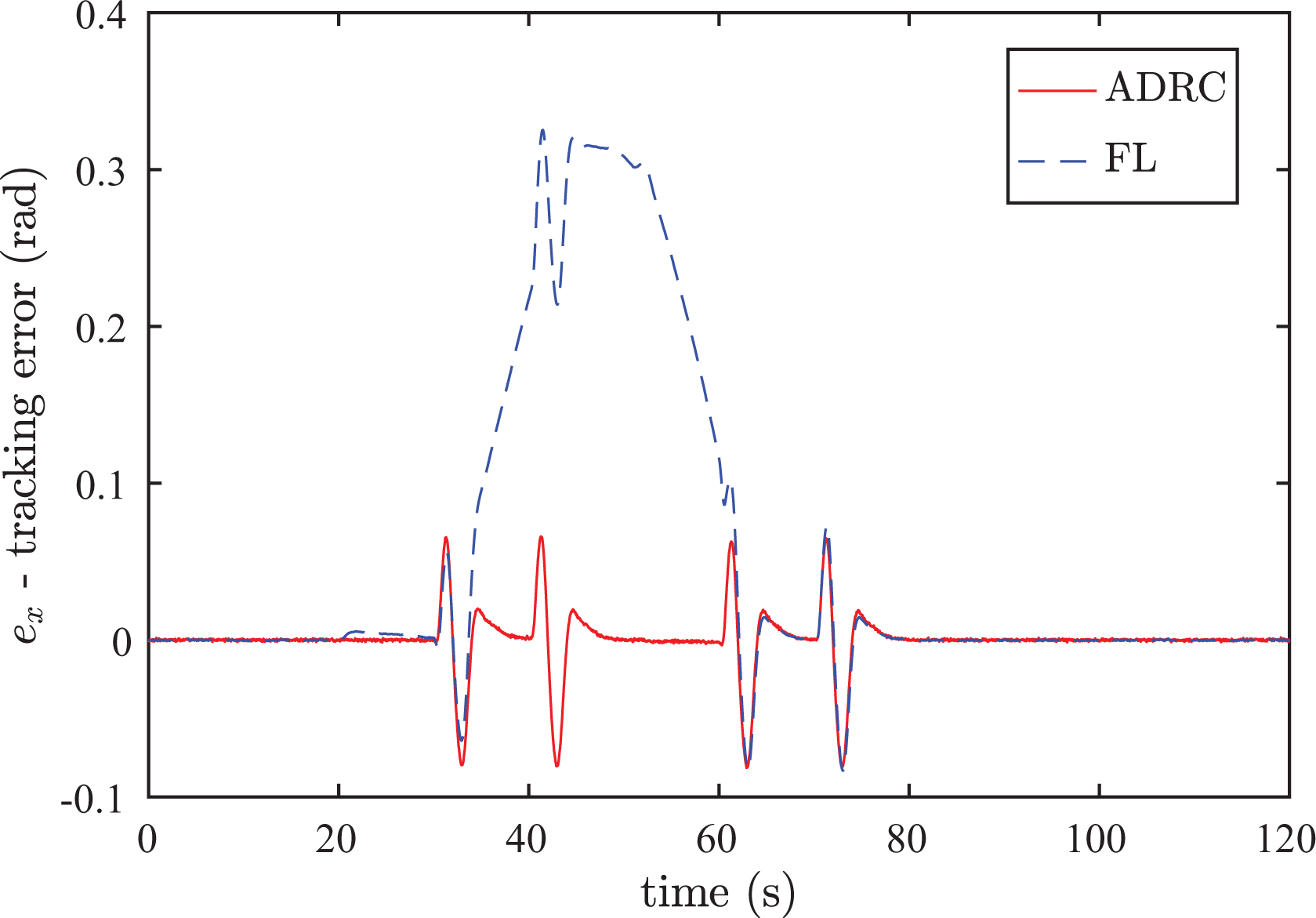
The control system is tested by means of simulations in MATLAB/Simulink environment. The mathematical model implemented for simulation is the standard one considered in the literature. The implementation of the controller is carried out taking into account the hybrid nonlinear observer briefly described above. The comparison is carried out for nominal parameters and in the presence of aerodynamic disturbances. The results are shown in Figures 4 to 11, and they are referred to two control laws, that is, the FL based on the analytical computation of the disturbance vector and the proposed control law based on the estimation of the disturbance vector, carried out by means of the ESOs. In particular, Figures 4 to 7 show the waveforms of the tracking errors of the coordinates of the center of gravity and the yaw angle with respect to the corresponding reference values. The forces generated by the four propellers corresponding to the considered experiment are shown in Figures 8 to 11. The results show the effectiveness of the proposed approach over the standard FL. In fact, with the proposed robust control law, the quadcopter tracks the trajectory with a high dynamic accuracy, whereas the standard FL control law produces tracking errors greater than those corresponding to the proposed robust control law. The simulation results confirm that the forces required to the propellers are effectively feasible. Finally, the simulation results show that the aerodynamic forces and moments are correctly estimated and compensated by the proposed control technique. Obviously, in the absence of aerodynamic forces and moments or other unknown endogenous disturbances, such as parametric uncertainties, the two control laws give the same results since the estimated disturbance vector is equal to the computed one.
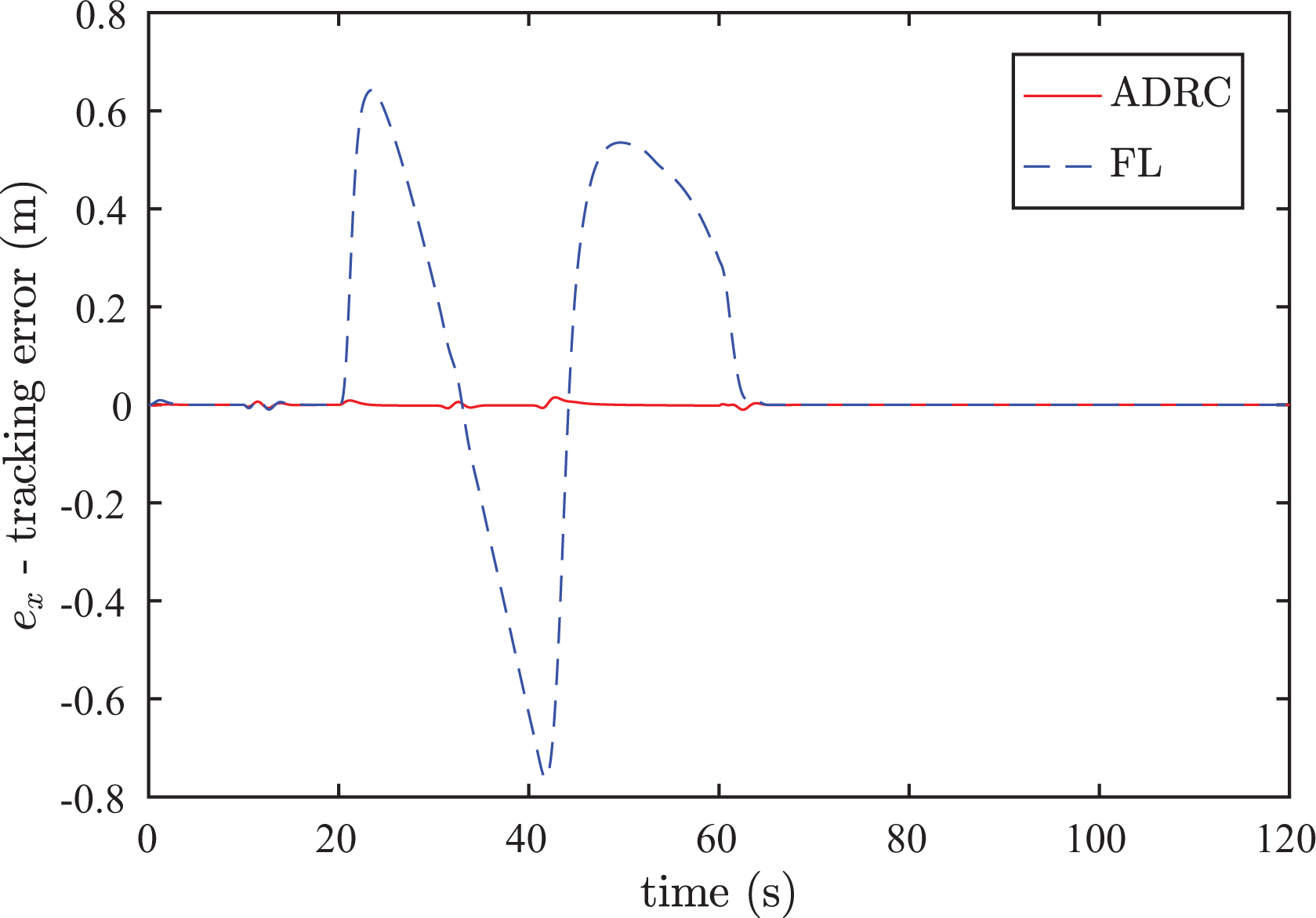
Tracking errors

Tracking errors

Tracking errors
Tracking errors

Force generated by the propeller 1 during the ADRC simulation experiment.

Force generated by the propeller 2 during the ADRC simulation experiment.

Force generated by the propeller 3 during the ADRC simulation experiment.

Force generated by the propeller 4 during the ADRC simulation experiment.
Conclusion
In this article, a systematic procedure is given for determining a robust motion control law for autonomous quadcopter vehicles. This procedure considers advanced control techniques, such as the input–output linearization and the ADRC. These techniques justify the use of the Brunovsky canonical form as the starting point for designing a controller for the motion control of the autonomous quadcopter. Then, it is possible to split the nonlinear augmented model into four decoupled models, three of which are of fourth order and one of second order. Starting from each of these models, it is possible to construct the relative ESO and to impose the dynamics to the model by means of pole assignment technique. As a final result, a robust control law is obtained, which outperforms the standard FL control.
While a quantitative expression of this performance improvement is not easy to be provided, the obtained simulation results highlight that a high decrease of the tracking errors during transients has been achieved. The reason for this is that the endogenous and exogenous disturbances have been considered as further state variables estimated by means of ESOs, permitting the nonlinearity of the plant and disturbances to be compensated. It follows that the proposed methodology could be considered as an “adaptive robust version” of the FL control technique since the state-feedback terms are estimated online. In this way, not only the problems due to the uncertainties on the parameters have been addressed but it is also possible to cope with unmodelled dynamics and exogenous disturbances (such as wind and aerodynamic disturbances). Simulation experiments, carried out on a Raspberry-PI board by means of the hardware-in-the-loop method, validate the approach followed in the article and show the better performance achieved with the proposed controller compared with the standard FL. The experimental validation of this methodology represents a future development to show the effectiveness of the proposed approach.
Supplemental material
Supplemental Material, sj-pdf-1-arx-10.1177_1729881421996974 - Trajectory robust control of autonomous quadcopters based on model decoupling and disturbance estimation
Supplemental Material, sj-pdf-1-arx-10.1177_1729881421996974 for Trajectory robust control of autonomous quadcopters based on model decoupling and disturbance estimation by Francesco Alonge, Filippo D’Ippolito, Adriano Fagiolini, Giovanni Garraffa and Antonino Sferlazza in International Journal of Advanced Robotic Systems
Footnotes
Declaration of conflicting interests
The author(s) declared no potential conflicts of interest with respect to the research, authorship, and/or publication of this article.
Funding
The author(s) received no financial support for the research, authorship, and/or publication of this article.
Supplemental material
Supplemental material for this article is available online.
Appendix 1
The elements of
with
The elements of
with
References
Supplementary Material
Please find the following supplemental material available below.
For Open Access articles published under a Creative Commons License, all supplemental material carries the same license as the article it is associated with.
For non-Open Access articles published, all supplemental material carries a non-exclusive license, and permission requests for re-use of supplemental material or any part of supplemental material shall be sent directly to the copyright owner as specified in the copyright notice associated with the article.