Sage Journals: Discover world-class research

Abstract

Unmanned aerial–aquatic vehicles are a new type of aircraft that can navigate in air and underwater. An unmanned aerial–aquatic rotorcraft (UAAR) is introduced to complete the task of navigating between air and underwater, and the trajectory optimization problem for this task is focused on in this study. The dynamics of a four-axle rotorcraft with eight rotors operating in air and underwater is described. On this basis, the trajectory optimization model is established, wherein the constraints on control variables and states in different media are included. The optimization index is denoted as the weighted sum of the terminal states. In view of the weakness of the teaching- and learning-based optimization (TLBO) algorithm, the formula for updating the individual grade in the teaching process is modified. Thus, this ensures that the algorithm avoids converging at the local optimum and improves the solution quality. Finally, an improved TLBO (ITLBO)-based trajectory optimization method for UAAR navigating between air and water is developed. The control variables are discretized with respect to height at a set of Chebyshev collocation points to reduce the terminal error of states, and the values of control variables at other heights are obtained via interpolation. In the simulation studies, the ITLBO-based method exhibits better performance in terms of optimizing the index when compared to the other two algorithms. Furthermore, the effects of the distribution and number of collocation points on the results are analyzed.

Keywords

Unmanned aerial–aquatic vehicle dynamics of rotorcraft different media trajectory optimization teaching- and learning-based optimization

Introduction

Unmanned aerial vehicles (UAVs) and autonomous underwater vehicles (AUVs) are increasingly attracting attention in recent years due to their wide range of applications in monitoring, inspection, and rescue.¹ UAVs can perform searching and shooting tasks in air, and AUVs can explore underwater topography and detect water quality.² The aerial and underwater vehicles are well adapted to their respective operating environments and can perform their assigned tasks satisfactorily.^3,4 However, in some scenarios, neither of the vehicles can perform tasks that require the capability of navigating in air and underwater. For example, during the inspection of the exterior of a submerged ship, a vehicle is required to navigate in air and underwater to locate the damage. An unmanned system composed of heterogeneous vehicles, such as UAV, unmanned surface vehicle, and AUV system, can perform such a task. However, the communication among the vehicles can become complicated.⁵ Besides, the structure of unmanned system composed of heterogeneous vehicles is more complicated, and the motion characteristics of heterogeneous vehicles are different. All the above factors will reduce the reliability of the whole system and decrease the efficiency of completing such tasks. Hence, an unmanned aerial–aquatic vehicle (UAAV) is appropriate for this type of assignment.

UAAVs can be classified into three categories based on the different functions, that is, aquatic UAAV, submarine-launched UAAV, and submersible UAAV.⁶ Systematic studies are mainly conducted on motion modeling and simulation of aquatic UAVs.⁷ Based on the classical potential flow theory and two-dimensional planar taxiing theory, the ski jump steering characteristics of aquatic UAVs were studied in reference,⁸ and the ski jump flight distance and thrust of UAV exhibit a significant effect on the ski jump trajectory. The motion model of an aquatic UAV was established, and simulations of takeoff cruise trajectory, stick-water taxiing trajectory, and contact-water skiing trajectory were performed.⁹ The analysis of the characteristics of various trajectories was also conducted.

When compared with aquatic UAVs and submarine-launched UAVs, submersible UAVs can autonomously navigate in air and underwater without relying on a platform. Hence, they can be applied in a wide range of applications.¹⁰ To date, submersible UAVs have been designed with three external shapes. The first shape consists of foldable wings, which are retracted during the water entry and underwater navigation to reduce drag.¹¹ The effects of the folding angle of the wing on the aerodynamic and hydrodynamic characteristics of UAAV were explored via wind and water tunnel experiments, and the motion model in air and underwater was established.¹² The second shape consists of a flapping wing, whose power is generated by the up–down oscillation of wings. The force and moment of the flapping-wing aircraft can be obtained via experiments.^13,14 Unlike the above two types of vehicles, navigation switchover between air and underwater is realized via multirotors.¹⁵

For a UAV, a unified control strategy is usually applied during the task, such as the varying cells strategy¹⁶ and the Markov decision process-based algorithm.¹⁷ To control the motion of UAAV, the common way is to design different strategies in the air and underwater, respectively. A multimode guidance strategy and a variable gain control system are put forward on the flying fish UAV in reference.¹⁸ The control system chooses the appropriate flight mode based on the rules of geometry and time to realize the navigation switchover. To avoid the complex switchover control strategy in the course of aerial–aquatic navigation, the process of aerial–aquatic switchover is regarded as an uncontrolled motion, during which the states of UAAV are determined entirely by its terminal state in the air, and then, the motion of UAAV is controlled after it has been entering water completely.¹⁹ The advantage of this strategy is that complex control system is not needed, and the instability caused by switchover between different control strategies is avoided. However, with the above control strategy, the desired trajectory of UAAV may not be generated as there are only several states which can be optimized. The various possibilities of trajectory are limited by only changing the initial states of entering water.

To this end, an unmanned aerial–aquatic rotorcraft (UAAR), which exhibits a simple structure and easy operation, is introduced to complete the task of navigating between air and underwater. The UAAR has fewer requirements on the takeoff and landing sites, and it is also capable of hovering at a fixed point, which is especially suitable for tasks requiring underwater photography and water quality monitoring. The trajectory of a UAAR can be controlled by changing the angular velocity of rotors. A UAAR is an eight-rotor vehicle. There is a paucity of studies that analyze the dynamic characteristic of such UAARs. Furthermore, when a UAAV navigates in air and underwater, the maximum angular velocity of a rotor changes with respect to different media. This should be considered when generating the trajectory of a UAAR. Swarm intelligence-based algorithms have been widely applied in solving various UAV trajectory optimization problems because they can obtain a satisfactory solution within a shorter computing time. Additionally, there are no special requirements on the model of the problem when compared to that in traditional algorithms, such as the indirect method and linear programming approach. Genetic algorithm, particle swarm optimization (PSO) algorithm, and ant colony optimization algorithm are the most popular swarm intelligence-based algorithms. With an increase in the number and types of problems, the drawbacks of classical algorithms are evident in different aspects, such as easily converging into a local optimum, slow convergence rate, and low solution quality. In recent years, new swarm intelligence-based algorithms are emerging considering the aforementioned drawbacks, and the teaching- and learning-based optimization (TLBO) algorithm demonstrated its superiority in many optimization problems. Specifically, the TLBO algorithm can be modified based on the characteristic of the established model to further improve its performance. The main contributions of this study are as follows:

A dynamic model of a UAAR is established by considering the characteristics of navigating from air to underwater. Different coordinates are used to describe the forces and moments imposed on a UAAR. Furthermore, equations that describe the motion of center of mass and rigid body are derived.

A mathematical model of trajectory optimization problem is developed. The constraint on the maximum angular velocity of rotor in different media is considered, and the UAAV is expected to hover after it dives in water. Furthermore, the terminal errors in position and velocity are included in the optimization index.

An improved TLBO (ITLBO) algorithm is proposed to optimize the angular velocity of each rotor. The best historical performance of an individual is considered when updating the individual grade in the teaching process. Chebyshev collocation points are set according to the height from the start point to the destination to optimize the angular velocities of rotors at those points.

Analysis on the motion characteristics of an unmanned aerial–aquatic rotorcraft

A dual-propeller UAAR is employed to conduct an underwater hovering mission.²⁰ The shape of the UAAR is shown in Figure 1.

Figure 1.

Sketch of the dual-propeller system.

As shown in Figure 1, two rotors are installed at the upper and lower ends of the axis, and they form two groups (group A and group B for convenience). Each group has four rotors. The two rotors on the same axis rotate in opposite directions to counteract the torque generated by the rotation of the other two rotors. During the process of the UAAR entering or leaving water, a steady aerial–aquatic navigation process is realized by adjusting the rotors’ speed. Furthermore, when entering water, the rotation speed of group A rotors is reduced to obtain a smooth transition of aerial–aquatic navigation. As group A rotors enter water and are increasingly away from the surface, the rotation speed of the rotors can be increased for normal navigation. Furthermore, as group B rotors enter water, they reduce the rotational speed. However, they increase the rotational speed when they are far from the surface. The rotational speeds of the two groups of rotors follow similar rules, as mentioned above, during the exit from water. It is extremely important to reduce the rotors’ speed near the water surface to avoid system instability due to sudden increase in drag during the complex process of aerial–aquatic motion.

Model for trajectory optimization for an underwater hovering task

After introducing the motion characteristics of a dual-propeller UAAR for aerial–aquatic navigation, it is necessary to establish the motion model of the UAAR. Furthermore, an index must be set to evaluate the completion of the task based on the constraints of an underwater hovering task.

Aerial–aquatic motion model of an unmanned aerial–aquatic rotorcraft

First, a coordinate system to describe the motion of the UAAR is established. Then, the simplification for aerial–aquatic motion is performed, as shown in Figure 2.

Figure 2.

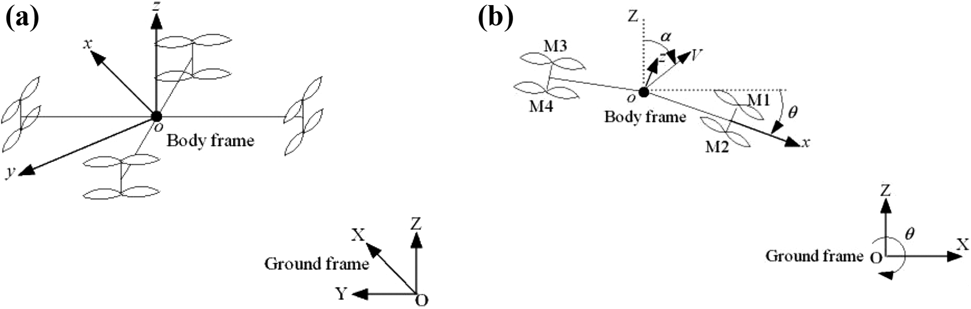
(a) Inertial frame and body frame describing the motion of the UAAR and (b) the simplification for navigating in different media. UAAR: unmanned aerial–aquatic rotorcraft.

In Figure 2(a), the Earth coordinate frame is fixed at any point on the horizontal plane and the body coordinate frame is fixed at the center of gravity of the UAAV. [X Y Z] and [x y z] denote the unit vectors of the positive directions of each axis of the Earth coordinate frame and body coordinate frame, respectively. The direction of ox axis is 45° with respect to the UAAR frame. In normal circumstances, the UAAR exhibits six degrees of freedom (DOF) for navigation. However, 3DOF is sufficient to complete the task of navigating from air to underwater. Furthermore, lateral motions, such as yaw and roll, should be avoided to ensure the stability of the UAAR during the transition between different media. It is difficult especially when the water is not calm. In this case, the moving water can be regarded as an external disturbance, which has an influence on the motion of UAAR, and a compensating controller is often designed to offset the force and moment caused by the moving water.²¹ As the navigation of UAAR between air and water is the main concern in this study, the motion of the UAAR in the xoz plane plays a leading role and is the focus, as shown in Figure 2(b). Specifically, M1, M2, M3, and M4 denote the four rotors, α denotes the angle of attack, and $θ$ denotes the pitch angle. The equations describing the motion of UAAR in xoz plane are shown in equations (1) to (3)

\ddot{X} = \frac{sin θ}{m} [2 K_{T} (ρ_{1} ω_{1}^{2} + ρ_{2} ω_{2}^{2} + ρ_{3} ω_{3}^{2} + ρ_{4} ω_{4}^{2})] + \frac{F_{d} sin α}{m}

\ddot{Z} = - g + \frac{cos θ}{m} [2 K_{T} (ρ_{1} ω_{1}^{2} + ρ_{2} ω_{2}^{2} + ρ_{3} ω_{3}^{2} + ρ_{4} ω_{4}^{2})] + \frac{F_{d} cos α}{m}

\ddot{θ} = 2 K_{T} d \frac{\sqrt{2}}{2} (- ρ_{1} ω_{1}^{2} - ρ_{2} ω_{2}^{2} + ρ_{3} ω_{3}^{2} + ρ_{4} ω_{4}^{2}) I_{y y}^{- 1}

In equations (1) to (3), m denotes the mass of UAAR and g denotes acceleration due to gravity, whose value is determined by the position of the UAAR ( $g_{air}$ and $g_{water}$ denote the acceleration of gravity in air and underwater, respectively). K_T denotes a value related to rotor pull coefficient (C_T ), which can be calculated as $K_{T} = A b^{2} C_{T}$ , where A denotes the area of the rotor and b denotes the radius of the rotor. Furthermore, $ρ_{i}$ and $ω_{i}$ (i = 1, 2, 3, 4) denote the density of the medium, where the rotor is located (denoted as $ρ_{air}$ and $ρ_{water}$ ), and angular velocity of the rotor, respectively. F_d denotes drag, which can be calculated as $F_{d} = C_{d} ρ A {(ω b)}^{2}$ , where C_d denotes the drag coefficient and $I_{y y}$ denotes the moment of inertia.

As shown in equations (1) to (3), it is evident that the state of UAAR can be obtained if the angular velocity of each rotor is provided. Although the 6DOF motion is not involved here, the angular velocity of each rotor still has an influence on the dynamics of UAAR.

Constraints on the underwater hovering task

The constraints on the underwater hovering task for the UAAR can be classified into the following two categories:

1. Constraints on control variables

The maximum angular velocity of the rotor is constrained by the limitation in the power of the motor and saturation and amplitude of actuators. The maximum angular velocity of a rotor of the UAAR is affected by air and water and changes with respect to the media. Additionally, when the rotor is close to the water surface, the angular velocity should be reduced, and it should be limited in a certain range to ensure the stability of aerial–aquatic motion. The aforementioned constraints are shown in Figure 3.

Figure 3.

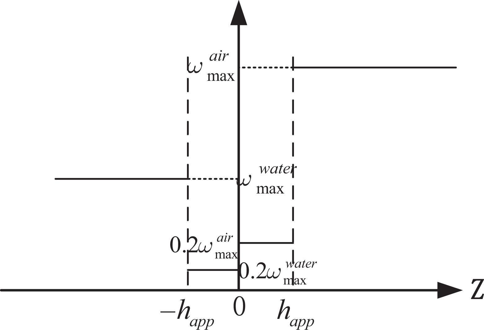
Constraints on angular velocity of rotor in different media.

In Figure 3, Z represents the height of the rotor from the water surface and $ω$ represents the angular velocity of the rotor. Specifically, $ω_{max}^{air}$ and $ω_{max}^{water}$ denote the maximum angular velocity of the rotor in air and underwater, respectively. Furthermore, $h_{app}$ denotes the critical value between the rotor and water surface. When the absolute distance between the rotor and water surface is less than this critical value, the maximum rotational speed can be allowed to decrease by 20% of the maximum in the corresponding medium to ensure the stability of motion.

2. State constraints in motion

During the process of diving into water, the pitch angle ( $θ$ ) of the UAAR should always be maintained at 0° to realize a smooth water entry, namely $θ (t) = 0^{\circ}$ . In this case, equations (1) to (3) are transformed as follows

\ddot{X} = 0

\ddot{Z} = - g + \frac{1}{m} [(2 K_{T} (ρ_{1} ω_{1}^{2} + ρ_{2} ω_{2}^{2} + ρ_{3} ω_{3}^{2} + ρ_{4} ω_{4}^{2})]

0 = - ρ_{1} ω_{1}^{2} - ρ_{2} ω_{2}^{2} + ρ_{3} ω_{3}^{2} + ρ_{4} ω_{4}^{2}

Equations (4) to (6) show that the UAAR only moves along the direction of Z axis in this task, and the rotors’ angular velocities satisfy the constraint in equation (6). Therefore, the state of the UAAR can be determined once $ω_{1}$ , $ω_{2}$ , and $ω_{3}$ are provided.

Optimization index for the underwater hovering task

The optimization index is used to evaluate the quality of the accomplishing assignments. In this task, the UAAR is required to reach the designated target point with a minimum terminal position error, and the ideal speed is set to 0 to complete the hovering task. The objectives can be expressed as follows

J = w_{1} \cdot | Z (t_{f}) - Z_{f} | + w_{2} \cdot | v (t_{f}) |

where J denotes the optimization index, w ₁ and w ₂ denote the weight coefficients of the terminal position error and velocity error, respectively. The two items in the optimization index correspond to the two requirements of reaching the target and hovering. These items can accurately describe the quality of finishing this task. Note that the item regarding the motion of UAAR in xoy plane is not included in equation (7) because in this task the motion along axis oz is the focus, and the corresponding motion equations are established. Besides, to ensure a vertical diving into water of UAAR, equations (4) to (6) must be satisfied, and the position of UARR in xoy plane stays the same during the diving process.

Principle and improvement of teaching- and learning-based optimization algorithm

After the mathematical model of this trajectory optimization problem is established, an optimization algorithm is required to search for an optimal trajectory. TLBO algorithm is a new swarm intelligence optimization algorithm that simulates the process of teachers’ teaching and students’ listening and learning to improve the academic performance of the whole class through the process of teaching and mutual learning of students.²² The advantage of TLBO algorithm is that the parameters are not set artificially. After establishing the mathematical model of the problem, the number of iterations is set to directly obtain the results. This ensures that the performance of the algorithm is not affected by the inappropriate parameter setting. However, TLBO algorithm exhibits the disadvantages of slow convergence and easily converging to a local optimum. Therefore, the quality of solution obtained via TLBO algorithm should be improved to promote the performance of the algorithm by considering the techniques used for the PSO algorithm as a reference. First, the basic principle and solving steps of TLBO algorithm are introduced, and then, the shortcomings of TLBO algorithm are improved.

Principles of teaching- and learning-based optimization algorithm

The class is taken as a unit, and the TLBO algorithm improves the learning performance of the whole class through teachers’ teaching and the mutual learning between students. In the algorithm, each individual (teacher or student) is regarded as a solution. The number of subjects, D, is treated as the dimension of the solution, and the class size, N, denotes the number of solutions, which are determined by the number of teachers and students. After introducing the aforementioned concepts, the steps of the TLBO algorithm are as follows.

1. Initialization

Set the initial score for each individual subject $S_{i} = (s_{i}^{1}, s_{i}^{2}, \dots, s_{i}^{D})$ , where (i = 1,2,…, N) in the class

s_{i}^{k} = s^{k_{L}} + rand \cdot (s^{k_{U}} - s^{k_{L}})

where k = 1, 2,…, D; $s^{k_{L}}$ and $s^{k_{U}}$ denote the lower limit and upper limit of the allowable score of subject k, respectively; and rand is a random number in the interval (0,1). By calculating the comprehensive performance of each individual (calculated using the indicator function of the problem), the individual with the best academic performance is designated as a teacher and recorded as $S_{teacher}$ .

2. Process of teacher’s teaching

Each student in the class learns according to the difference between the average academic performance of teachers and students. They compare the comprehensive academic performance of each student before and after learning. If the latter is better, then they update their own results. The learning process can be expressed in equation (9) as follows

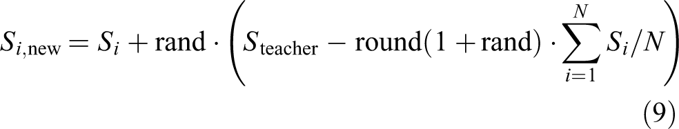
S_{i, new} = S_{i} + rand \cdot (S_{teacher} - round (1 + rand) \cdot \sum_{i = 1}^{N} S_{i} / N)

In equation (9), round is used to round a decimal to the nearest integer. After updating the performance with equation (9), the better solution between $S_{i, new}$ and S_i is set as the final result.

3. Mutual learning among students

Each student (S_i ) randomly chooses two different learning objects (S_i and S_k , i $\neq$ j $\neq$ k) in the class. Student S_i learns through the difference between S_i and S_k . At the end of the study, the comprehensive results of each student before and after learning are compared. If the latter is better, then their respective results are updated. The learning process can be expressed as follows

S_{i, new} = \{\begin{matrix} S_{i} + rand \cdot (S_{j} - S_{k}), S_{j} superior to S_{k} \\ S_{i} + rand \cdot (S_{k} - S_{j}), S_{k} superior to S_{j} \end{matrix}

After updating the performance with equation (10), the better solution between $S_{i, new}$ and S_i is set as the final result.

4. Update of the teacher, continue iterative processes, or end algorithms

The teacher is designated as the individual with the best comprehensive performance in the class at this time of iteration.

5. Judgement whether the terminal condition of algorithm is satisfied

If the terminal condition of the algorithm is not satisfied, then the iterative process from steps 2 to 4 will be continued. Otherwise, the algorithm is terminated, and the teacher’s learning results are output as the optimal solution.

The process of updating an individual’s performance in class in TLBO algorithm is similar to that of updating a particle’s position in PSO algorithm. Both algorithms use a global optimal solution to update individual information. Unlike PSO algorithm, TLBO algorithm updates individual information using average individual academic performance and communicating between students, which can maintain the diversity of individual classes. Hence, it is not easy to converge to a local optimum.

Improvements in teaching- and learning-based optimization algorithm

The discussion in “Aerial–aquatic motion model of an unmanned aerial–aquatic rotorcraft” section demonstrates that TLBO algorithm is less likely to converge to a local optimum than PSO. However, in TLBO algorithm, individual information is updated with an individual’s average score, which can lead to the incomplete description of students’ academic performance and in turn affect the quality of solutions.

Based on the idea of the PSO algorithm, where individual historical optimal solution is utilized to update the position of particles,²³ an individual historical optimal solution is adopted as opposed to an individual average score to update individual performance in the teaching process of teachers in TLBO algorithm. Thus, equation (9) can be transformed as follows

S_{i, new} = S_{i} + rand \cdot (S_{teacher} - round (1 + rand) \cdot S_{i, best})

where $S_{i, best}$ denotes the historical optimal performance of individual i. In this manner, the global optimal information, individual historical optimal information, and information exchanged between individuals are applied while an individual’s academic performance is updated. This ensures that TLBO algorithm does not easily converge to a local optimum in the process of solving and improving the quality of solution.

Trajectory optimization of unmanned aerial–aquatic rotorcraft for navigating between air and water based on improved teaching- and learning-based optimization algorithm

In “Principle and improvement of teaching- and learning-based optimization algorithm” section, the principles of TLBO algorithm and its improvement are described without combining any application of the algorithm. In this section, the trajectory optimization problem of UAAR for navigating between air and water will be solved based on ITLBO algorithm, and the detailed procedures will be elaborated. First, the line segments between the initial and final altitudes of UAAR are discretized into a certain number of Chebyshev collocation points. Only the control variables at Chebyshev points are optimized, and the values of control variables at other altitudes can be obtained via interpolation. Then, the trajectory optimization problem of UAAR can be transformed into the process of optimizing the control variables, which can be solved by ITLBO algorithm. The optimization variables and the constraints are formulated into ITLBO algorithm considering the real situation of navigating between air and water.

Generation of Chebyshev collocation points

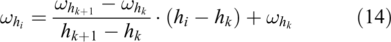
The collocation points are generated by the Chebyshev pseudospectral method.²⁴ Collocation points are distributed based on the value of altitude coordinates. The specific calculation is shown in equation (12)

Z_{k} = cos (\frac{(n - k) \cdot π}{n}) (k = 0, 1, 2, \dots, n)

The number of collocation points is n+1 (including two endpoints) and Z_k denotes the height of the k’th collocation points. Equation (12) shows that Chebyshev collocation points are dense at both ends and sparse in the middle, which are appropriate for addressing the constraints on terminal position and velocity in this problem. (More control variables at the end can be optimized to easily satisfy the terminal constraints.) It is important to note that the value of $Z_{k} \in [- 1, 1]$ in equation (12) should be converted to interval [Z_s , Z_f ] to satisfy the requirements of the problem. The conversion equation is shown in equation (13)

h_{k} = \frac{Z_{f} - Z_{s}}{2} \cdot Z_{k} + \frac{Z_{f} + Z_{s}}{2}

where h_k (k = 0, 1,…, n) denotes the collocation points in this problem. The trajectory of diving into water and hovering underwater can be obtained by optimizing the control variables at these points. The reason for selecting altitude as opposed to moving time as the allocation points is that the restrictions due to angular velocity of the rotor, medium density, and gravitational acceleration on the UAAR vary with altitude. If the allocation points are divided based on the moving time, then the aforementioned variables cannot be judged intuitively based on the altitude of the UAAR. Although the altitude of UAAR can be calculated by the equations of motion, it increases the computational complexity.

Operation on control variables

The angular velocities of four rotors are the control variables to determine the trajectory of UAAR in this problem. Hence, the angular velocity of the remaining rotors can be solved by equation (6) if the angular velocities of three rotors are determined. Let $ω_{1}$ , $ω_{2}$ , and $ω_{3}$ denote the control variables. The values of the control variables at the collocation points are determined in “Generation of Chebyshev collocation points” section, while the values of the control variables at the other heights are not known. In this study, the linear interpolation method is utilized to determine the values of control variables at the remaining heights between two adjacent collocation points, as shown in equation (14)

ω_{h_{i}} = \frac{ω_{h_{k + 1}} - ω_{h_{k}}}{h_{k + 1} - h_{k}} \cdot (h_{i} - h_{k}) + ω_{h_{k}}

where $h_{k} > h_{i} > h_{k + 1}$ and $ω_{h_{i}}$ can be calculated by equation (14) after $ω_{h_{k}}$ and $ω_{h_{k + 1}}$ are determined.

Solution procedures of underwater fixed-point hovering trajectory optimization

The following steps are taken to solve the trajectory optimization problem for a UAAR underwater fixed-point hovering:

Initialize the maximum number of iterations I, class size N, and the number of Chebyshev collocation points D (i.e. the number of disciplines learned by each individual in the TLBO algorithm). The rotation angular velocities of rotors M1, M2, and M3 at each collocation point are initialized under the constraints of maximum rotation angular velocities in different media, and the corresponding rotation angular velocity of rotor M4 is calculated according to equation (6). It is important to note that if the rotation angular velocity of rotor M4 does not satisfy the requirement of the maximum rotation angular velocity, then the rotation angular velocities of rotors M1, M2, and M3 should be reinitialized until M4 satisfies the constraint of maximum rotation angular velocity.

Calculate fitness values of N individuals with equation (7) separately. Select the individuals with the lowest fitness values as teachers and the others as students. Record the global optimal solution and historical optimal solution of each individual.

Enter the iteration process, update the individual information with equation (11), and compare the fitness values of each individual before and after learning. If the fitness values after learning are smaller, then update the fitness values with the smaller value.

Update individual information with equation (10) and compare the fitness values of each individual before and after learning. If the fitness function values after learning are smaller, then update the fitness values with the smaller value.

Update the global optimal solution and individual’s historical optimal solution and designate the individual with the current global optimal solution as a teacher. Judge whether the number of iterations reaches the specified maximum number. If the answer is yes, then stop the calculation and output the current global optimal solution as the result; otherwise, proceed to step 3 again.

The above steps can be represented by an algorithm flowchart, as shown in Figure 4.

Figure 4.

Flowchart of the trajectory optimization problem for a UAAR hovering underwater. UAAR: unmanned aerial–aquatic rotorcraft.

The blue box in Figure 4 shows the improvements in the TLBO algorithm. After obtaining the global optimal solution, the time histories of angular velocities of rotors are inputted to the established dynamic model to calculate the states of UAAR at each moment.

Simulation and analysis of results

To illustrate the feasibility of the proposed trajectory optimization method for underwater hovering of UAAR based on ITLBO algorithm, three sets of simulation experiments are conducted in this study. In the first group of experiments, PSO, TLBO, and ITLBO algorithms are used to solve the underwater hovering trajectory optimization problem, and the simulation results of different algorithms are compared. In the second and third group of experiments, the impact of the distribution and the number of collocation points on the experimental results are explored, respectively. The experimental parameters are listed in Table 1, and the parameters related to the motion model of the dual-propeller UAAR are listed in Table 2.²⁵ The parameters of PSO algorithm are taken from a previous study.²⁶

Table 1.

Parameters for the simulations.

Parameters	w ₁	w ₂	N	D	I	Z_s (m)	Z_f (m)
Values	0.5	0.5	100	34	50	1	−2

Table 2.

Parameters for the motion of UAAR.

Parameters	Values	Units
M	2	kg
K_T	1.34 × 10⁻⁵	m⁴/rad
$ρ_{air}$	1.225	kg/m³
$ρ_{water}$	999.97	kg/m³
$g_{air}$	9.81	m/s²
$g_{water}$	0.35	m/s²
$ω_{max}^{air}$	773.1	rad/s
$ω_{max}^{water}$	23.25	rad/s
$h_{app}$	0.1	m

UAAR: unmanned aerial–aquatic rotorcraft.

Comparison among different algorithms

Based on the parameters in Tables 1 and 2, PSO, TLBO, and ITLBO algorithms are adopted to solve the underwater hovering trajectory optimization problem. The fitness values are varied with respect to the number of iterations, as shown in Figure 5.

Figure 5.

Fitness values for three different algorithms.

In Figure 5, the fitness function value obtained via ITLBO algorithm is the smallest, and the convergent speed is the fastest. However, the result obtained via PSO algorithm is the worst among the three algorithms. To show the final fitness value more clearly, the corresponding terminal height and final speed of UAAR in three algorithms are given in Table 3.

Table 3.

Final fitness values, height, and velocity.

Algorithm	Fitness function final value	Z(t_f ) (m)	V(t_f ) (m/s)
PSO	0.7223	−0.5553	−6.0407 × 10⁻⁵
TLBO	0.0281	−1.9447	−0.0010
ITLBO	7.2284 × 10⁻⁴	−2.0006	−8.2747 × 10⁻⁴

PSO: particle swarm optimization; TLBO: teaching- and learning-based optimization; ITLBO: improved teaching- and learning-based optimization.

As provided in Table 3, PSO algorithm exhibits the best performance in hover with the lowest terminal speed. However, the terminal height differs significantly from the ideal height of −2 m. The final fitness value obtained by the ITLBO algorithm is lower than those of the other two algorithms by over two orders of magnitude, and the quality of trajectory is enhanced by 99.8% and 97.4% when compared to those of PSO and TLBO algorithms, respectively. Figures 6 to 8 show the time-varying plots of height, velocity, and angular velocity of the rotor of UAAR for the three algorithms.

Figure 6.

Height of UAAR with respect to three different algorithms. UAAR: unmanned aerial–aquatic rotorcraft.

Figure 7.

Velocity of UAAR with respect to three different algorithms. UAAR: unmanned aerial–aquatic rotorcraft.

Figure 8.

Angular velocity of rotors with respect to three different algorithms.

To verify whether the maximum number of iterations affects the simulation results, I = 100, 200, 300 is set. The simulation experiments are implemented with PSO and ITLBO algorithms. The time-varying plots of fitness values are obtained, as shown in Figure 9. The corresponding final fitness values, terminal height, and final velocity are listed in Table 4.

Figure 9.

Fitness values with respect to different maximum times of iteration.

Table 4.

Final fitness values, height, and velocity with respect to different maximum times of iteration.

Algorithm	Final fitness value	Z(t_f ) (m)	V(t_f ) (m/s)
PSO (I = 100)	0.5068	−0.981	−7.9518 × 10⁻⁴
PSO (I = 200)	0.3218	−1.3824	−0.0260
PSO (I = 300)	0.0078	−1.9843	−2.4634 × 10⁻⁵
ITLBO (I = 100)	6.5394 × 10⁻¹³	−2.0000	−2.9203 × 10⁻¹³

As shown in Figure 9 and Table 4, the final fitness values of PSO and ITLBO algorithms decrease as the maximum number of iterations increases. This indicates an improvement in the quality of solutions that are obtained. Specifically, with respect to ITLBO algorithm, when I = 100, the terminal height and terminal velocity are very close to the ideal value, which can completely satisfy the requirements of fixed-point hovering underwater.

As shown in the simulation results, the proposed trajectory optimization method based on ITLBO algorithm can completely satisfy the requirements of an accurate underwater fixed-point hovering task. Furthermore, the proposed method is superior to PSO and TLBO algorithms in terms of convergent speed and solution quality.

Influence of different distribution of collocation points on the simulation results

In “Comparison among different algorithms” section, Chebyshev collocation points are adopted in the simulation. To further explore the effect of different collocation point distribution on the simulation results, Lagrange–Gauss (L-G) collocation points and uniformly distributed collocation points are utilized in this section. The simulation results are compared with those obtained by Chebyshev collocation points. The parameters in Tables 1 and 2 are still used in the simulation, and ITLBO algorithm is adopted. The distribution of L-G collocation points can be obtained from the root of the following K’th Lagrange polynomial (equation (14))²⁷

P_{K} (\bar{τ}) = \frac{1}{2^{K} \cdot K!} \cdot \frac{d^{K}}{d {\bar{τ}}^{K}} \cdot [{({\bar{τ}}^{2} - 1)}^{K}], K = 0, 1, 2...

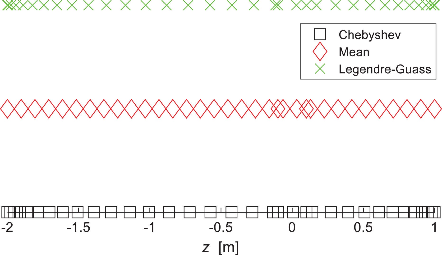
Equation (15) is solved at the collocation point $\bar{τ} \in [- 1, 1]$ , where equation (13) is required to convert the collocation points to the values between the beginning and end of the height of UAAR. The distribution rules of the three types of collocation points are shown in Figure 10.

Figure 10.

Distributions of Chebyshev mean and Legendre–Gauss collocation points.

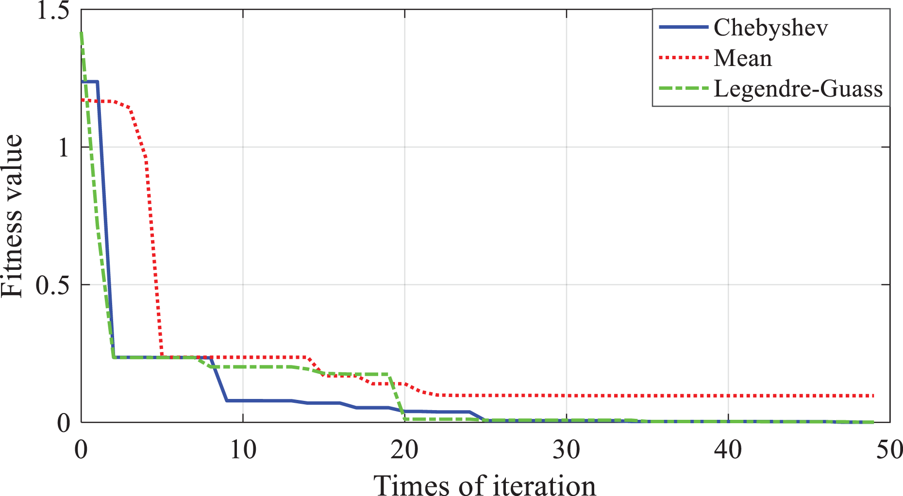
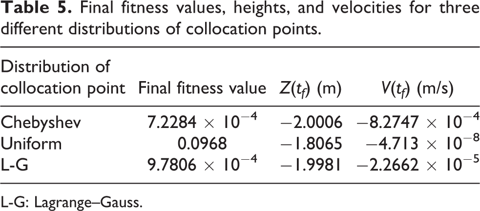
It is important to note that two corresponding points h _app and −h _app are also added to the collocation points. Hence, the points in Figure 10 are not completely symmetrical. The fitness values obtained by adopting the above collocation points distribution are shown in Figure 11, and the corresponding information in Figure 10 is given in Table 5.

Figure 11.

Fitness values for three different distributions of collocation points.

Table 5.

Final fitness values, heights, and velocities for three different distributions of collocation points.

Distribution of collocation point	Final fitness value	Z(t_f ) (m)	V(t_f ) (m/s)
Chebyshev	7.2284 × 10⁻⁴	−2.0006	−8.2747 × 10⁻⁴
Uniform	0.0968	−1.8065	−4.713 × 10⁻⁸
L-G	9.7806 × 10⁻⁴	−1.9981	−2.2662 × 10⁻⁵

L-G: Lagrange–Gauss.

As shown in Figure 11 and Table 5, the three distribution modes exhibit slight effect on the convergent rate of ITLBO algorithm, but the results of utilizing Chebyshev and L-G collocation points are better than that of uniformly distributed collocation points. In Figure 10, Chebyshev collocation points and L-G collocation points exhibit the characteristics of sparse middle and dense two ends, that is, they can control the terminal navigation state more accurately. However, the uniformly distributed collocation point does not exhibit this characteristic.

Influence of the number of different collocation points on the simulation results

The number of collocation points determines the number of variables that should be optimized in the optimization problem, and this also affects the simulation results. In this section, the parameters in Tables 1 and 2 are adopted to solve the same trajectory optimization problem with ITLBO algorithm under the distribution of Chebyshev collocation points. The number of collocation points is set as D = 14, 34, 54, as shown in Figure 12.

Figure 12.

Diagram of different collocation points (D = 14, 34, 54).

With respect to D = 14, 34, 54, the fitness values obtained by varying the number of iterations are shown in Figure 13, and the corresponding information in Figure 13 is given in Table 6.

Figure 13.

Fitness values with respect to the number of collocation points.

Table 6.

Final fitness values, heights, and velocities with respect to the number of collocation points.

Number of collocation point	Final fitness value	Z(t_f ) (m)	V(t_f ) (m/s)
D = 14	0.0270	−2.0181	0.0359
D = 34	7.2284 × 10⁻⁴	−2.0006	−8.2747 × 10⁻⁴
D = 54	0.0065	−2.0035	0.0094

As shown in Figure 13 and Table 6, the number of collocation points slightly affects the convergent speed of ITLBO algorithm. When the number of collocation points is low (D = 14), the computational load of the algorithm correspondingly reduces. Due to the insufficient number of controllable variables, the UAAR cannot obtain the desired terminal state. When the number of collocation points is high (D = 54), the aforementioned situation is improved. However, the computational load of the algorithm increases exponentially as the number of collocation points increases. Based on the premise of a certain class size (N) and a maximum number of iterations (I), the number of collocation points increases the number of possible combinations of solutions, which reduces the probability of obtaining the optimal solution. Therefore, D = 34 is the appropriate number of collocation points, which is consistent with the scale and characteristics of the problem. Hence, extremely few or too many collocation points lead to a solution that deviates from the optimal solution.

Conclusions

In this article, the trajectory optimization problem of a UAAR in an underwater hovering task is examined, and the task involves complete navigation of the UAAR from air to underwater. First, the motion characteristics of a dual-propeller UAAR in aerial–aquatic navigation are described, and the dynamic equations of UAAR are derived. The mathematical model of trajectory optimization is established by considering the constraints on the angular velocity of the rotor in different media and the states of UAAR in the underwater hovering task. The goal is to minimize the weighting sum of terminal error of position and velocity of the UAAR. To solve the established model, an ITLBO algorithm is proposed to overcome the shortcomings of TLBO algorithm in updating an individual’s learning performance in the teaching stage, and the individual historical optimal solution is introduced to improve the individual learning performance. Based on ITLBO algorithm, the trajectory optimization algorithm for the underwater hovering task is developed. In the algorithm, Chebyshev collocation points are used to determine the discrete heights that should be optimized. This is beneficial for realizing an accurate control of the terminal states. Furthermore, simulation results demonstrate that the proposed ITLBO-based trajectory optimization method for underwater hovering task of the UAAR is valid, and it is superior to PSO and TLBO algorithms in terms of optimizing the proposed index. Additionally, the distribution and quantity of collocation points affect the simulation results. In future studies, a real experimental platform referring to the literature²⁵ can be developed to test the validity of the proposed algorithm, and new tasks can be added to extend its function. It is difficult and many unexpected factors must be integrated together. Besides, the disturbance caused by the motion of water can be considered in real situations, and a robust compensating controller is expected to be designed to deal with the issue.

Footnotes

Acknowledgments

We express our heartfelt thanks to Chongqing Research Program of Basic Research and Frontier Technology, Fundamental Research Funds for the Central Universities, and China Scholarship Council.

Declaration of conflicting interests

The author(s) declared no potential conflicts of interest with respect to the research, authorship, and/or publication of this article.

Funding

The author(s) disclosed the following financial support for the research, authorship, and/or publication of this article: This research work was financially supported by the Chongqing Research Program of Basic Research and Frontier Technology with the grant number of cstc2020jcyj-msxmX0602, Fundamental Research Funds for the Central Universities with the project reference number of 2020CDJ-LHZZ-066, and China Scholarship Council with the project reference number of 201906055030.

ORCID iD

Yu Wu

References

Hui

Bian

Zhao

, et al. A monocular-based navigation approach for unmanned aerial vehicle safe and autonomous transmission-line inspection. Int J Adv Robot Syst 2019; 16(1). DOI: 10.1177/1729881419829941.

Paull

Saeedi

Seto

, et al. AUV navigation and localization: a review. IEEE J Ocean Eng 2013; 39(1): 131–149.

Al-Mousa

Sababha

Al-Madi

, et al. UTSim: a framework and simulator for UAV air traffic integration, control, and communication. Int J Adv Robot Syst 2019; 16(5): 1729881419870937.

Murphy

Steimle

Griffin

, et al. Cooperative use of unmanned sea surface and micro aerial vehicles at Hurricane Wilma. J Field Robot 2008; 25(3): 164–180.

Low

. Cooperative path planning for heterogeneous unmanned vehicles in a search-and-track mission aiming at an underwater target. IEEE Trans Veh Technol 2020; 69(6): 6782–6787.

Yang

Liang

Wen

, et al. Research status of water-air amphibious trans-media unmanned vehicle. Robot 2017; 40(1): 102–114.

Feng

Yang

. Research on vertical air–water trans-media control of hybrid unmanned aerial underwater vehicles based on adaptive sliding mode dynamical surface control. Int J Adv Robot Syst 2018; 15(2): 1729881418770531.

Wang

Zhang

Zhu

. Simulation and analysis on Ballistic trajectory of trans-media aircraft. Comput Simul 2011; 28(12): 1–4.

Yang

. Modeling and simulation of dynamic characteristics of slide jump steering trajectory for trans-media UAV. Torpedo Technol 2012; 20(6): 401–406.

10.

Yang

Wang

Liang

, et al. Survey on the novel hybrid aquatic–aerial amphibious aircraft: aquatic unmanned aerial vehicle (AquaUAV). Prog Aerosp Sci 2015; 74: 131–151.

11.

Siddall

Kovač

. Launching the AquaMAV: bioinspired design for aerial–aquatic robotic platforms. Bioinspir Biomim 2014; 9(3): 031001.

12.

Siddall

Ortega Ancel

Kovač

. Wind and water tunnel testing of a morphing aquatic micro air vehicle. Interf Focus 2017; 7(1): 20160085.

13.

Lock

Vaidyanathan

Burgess

, et al. Development of a biologically inspired multi-modal wing model for aerial-aquatic robotic vehicles through empirical and numerical modelling of the common guillemot, Uria aalge. Bioinspir Biomim 2010; 5(4): 046001.

14.

Liang

Yang

Wang

, et al. Design and experiment of a bionic gannet for plunge-diving. J Bionic Eng 2013; 10(3): 282–291.

15.

Drews

Neto

Campos

. Hybrid unmanned aerial underwater vehicle: modeling and simulation. In: 2014 IEEE/RSJ international conference on intelligent robots and systems, Chicago, IL, USA, 14–18 September 2014, pp. 4637–4642. USA: IEEE.

16.

Zhou

Peng

. UAV collision avoidance based on varying cells strategy. IEEE Trans Aerosp Electr Syst 2018; 55(4): 1743–1755.

17.

Zhou

Zhang

. Collision-free trajectory generation and tracking for UAVs using Markov decision process in a cluttered environment. J Intell Robot Syst 2019; 93(1): 17–32.

18.

Eubank

Atkins

Macy

. Autonomous guidance and control of the flying fish ocean surveillance platform. In: AIAA infotech@ aerospace conference and AIAA unmanned…unlimited conference, Seattle, Washington, 6–9 April 2009, p. 2021. USA: American Institute of Aeronautics and Astronautics.

19.

, et al. Dynamics modeling and trajectory optimization for unmanned aerial-aquatic vehicle diving into the water. Aerosp Sci Technol 2019; 89: 220–229.

20.

Ravell

DAM

Maia

Diez

. Modeling and control of unmanned aerial/underwater vehicles using hybrid control. Control Eng Pract 2018; 76: 112–122.

21.

Svacha

Mohta

Kumar

. Improving quadrotor trajectory tracking by compensating for aerodynamic effects. In: 2017 international conference on unmanned aircraft systems (ICUAS). Miami, FL, USA, 13–16 June 2017, pp. 860–866. USA: IEEE.

22.

Rao

Savsani

Vakharia

. Teaching–learning-based optimization: an optimization method for continuous non-linear large scale problems. Inform Sci 2012; 183(1): 1–15.

23.

Kennedy

Particle swarm optimization. Encyclopedia of machine learning, Boston: Springer, 2010, pp. 760–766.

24.

. A general trajectory optimization method for aircraft taxiing on flight deck of carrier. Proc Instit Mech Eng Part G: J Aerosp Eng 2019; 233(4): 1340–1353.

25.

Maia

Soni

Diez

. Demonstration of an aerial and submersible vehicle capable of flight and underwater navigation with seamless air-water transition. 2015; arXiv preprint arXiv:1507.01932.

26.

Shi

Eberhart

. Parameter selection in particle swarm optimization. In: International conference on evolutionary programming, San Diego, California, USA, March 25–27, 1998, pp. 591–600. Berlin, Heidelberg: Springer.

27.

. Chicken swarm–based method for ascent trajectory optimization of hypersonic vehicles. J Aerosp Eng 2017; 30(5): 04017043.

Trajectory optimization of an unmanned aerial–aquatic rotorcraft navigating between air and water

Abstract

Keywords

Introduction

Analysis on the motion characteristics of an unmanned aerial–aquatic rotorcraft

Model for trajectory optimization for an underwater hovering task

Aerial–aquatic motion model of an unmanned aerial–aquatic rotorcraft

Constraints on the underwater hovering task

Optimization index for the underwater hovering task

Principle and improvement of teaching- and learning-based optimization algorithm

Principles of teaching- and learning-based optimization algorithm

Improvements in teaching- and learning-based optimization algorithm

Trajectory optimization of unmanned aerial–aquatic rotorcraft for navigating between air and water based on improved teaching- and learning-based optimization algorithm

Generation of Chebyshev collocation points

Operation on control variables

Solution procedures of underwater fixed-point hovering trajectory optimization

Simulation and analysis of results

Comparison among different algorithms

Influence of different distribution of collocation points on the simulation results

Influence of the number of different collocation points on the simulation results

Conclusions

Footnotes

Acknowledgments

Declaration of conflicting interests

Funding

ORCID iD

References