Sage Journals: Discover world-class research

Abstract

Position–velocity–time control mode has been wildly used in industrial application. And velocity planning is one of the most important factors to determine the performance of position–velocity–time motion. To generate smooth trajectory while satisfying the kinematic constraints of the devices such as the maximum velocity, acceleration, and jerk, a novel velocity planning method is proposed. Firstly, a modified S-shaped acceleration/deceleration algorithm is designed to restrict the kinematic parameters. Meanwhile, a series of rules are specified to constrain the velocity profile to simplify the velocity planning process. On this basis, the velocity planning method is proposed based on the modified acceleration/deceleration algorithm. For reasonable position–velocity–time command, the given position–velocity–time conditions can be satisfied with smooth velocity profile, where the kinematic parameters can be limited in their allowable ranges. For unreasonable position–velocity–time commands, a series of planning strategies are designed to adjust the given conditions according to the user needs, which is suitable for the real application. The comparative experiments show that the proposed method can realize the velocity planning for position–velocity–time motion with smooth trajectory while restricting the kinematic parameters. The computational load is also tested to satisfy the real-time requirement. Therefore, the proposed velocity planning method has good performance and strong practicability.

Keywords

Position–velocity–time (PVT) control smooth trajectory velocity planning modified S-shaped ACC/DEC algorithm kinematic constraints

Introduction

Position–velocity–time (PVT) control mode, where the motion axes can get to the specified position with desired velocity and time, has been wildly used in motion control.^1,2 In that mode, the controller conducts the velocity planning according to a series of points with PVT information which are called PVT commands. Compared with the position–velocity (PV) and position–time (PT) control modes, PVT mode has a stronger constraint on motion process. However, in some application situations, the PVT commands are send by the host computer with a certain beat rather than obtained by velocity look ahead. Hence, the given conditions might not match to the kinematic constraints of the devices such as the maximum velocity, acceleration, and jerk, which affects the motion smoothness and might cause damage to the drive and transmission components. Therefore, it is critical to develop an appropriate velocity planning method to guarantee the motion smoothness while restricting the motion parameters.

The most common used velocity planning methods for PVT control are cubic and quintic polynomial interpolation algorithms.^2

–7 Each PVT command is used as the planning interval to construct the trajectory by cubic or quintic polynomial functions. And the conditions of PVT command at the end of command interval can always be satisfied. Meanwhile, polynomial interpolation algorithms is easy to conduct with small computational load.

However, the acceleration profiles obtained by the cubic polynomial method are discontinuous at the edges of each interval. Meanwhile, the Runge phenomenon⁸ is obvious with the fifth-order polynomial function in some situations, which causes serious oscillations. Moreover, the velocity, acceleration, and jerk profiles in each interval obtained by polynomial methods are uncontrollable and might exceed the kinematic constraints, which might cause damage to devices and affect motion accuracy.

To restrict the motion parameters, various acceleration/deceleration (ACC/DEC) algorithms can be used. Some jerk-limited ACC/DEC algorithms such as the S-shaped method^9
–11 and the dynamic jerk constraint method¹² have been employed to generate continuous acceleration profile. To simplify the expression and calculation process of polynomial methods, some trigonometric ACC/DEC algorithms are developed such as the Sine-curve methods.^13,14 However, the motion efficiency is limited because the maximum velocity, acceleration, or jerk cannot be maintained in these trigonometric methods.¹⁵ To further improve the motion smoothness, some jerk-continuous ACC/DEC algorithms^16

–19 are proposed. However, their expressions and the computation process of velocity planning are complicated.

Among these algorithms, the S-shaped ACC/DEC has continuous acceleration and limited jerk^20,21 which is necessary and sufficient for smooth trajectory. Meanwhile, the specified rules with seven sections have strong constraint ability on kinematic parameters.^22,23 In addition, the calculation process of velocity planning is simple and standard.²⁴ However, the typical S-shaped ACC/DEC algorithm and the corresponding velocity planning method cannot consider the motion time condition, which cannot be used to PVT application directly and needs to be modified.

To cope with these problems, a velocity planning method is proposed in this paper for PVT control. The main contributions can be described as follows:

A modified S-shaped ACC/DEC algorithm is designed based on the typical algorithm, which can consider the time condition and maintain the properties in terms of smoothness, simplicity, and ability to constrain the kinematic parameters.

On this basis, a series of rules are specified to restrict the form of velocity profile to simplify the velocity planning process.

The velocity planning method is proposed base on the modified ACC/DEC algorithm. By the proposed method, smooth trajectory can be generated to satisfy the given PVT conditions while the kinematic parameters are restricted within their given ranges, which is suitable for the real application.

The remainder of this article is organized as follows. In the second section, the typical S-shaped ACC/DEC algorithm and its modification are illustrated. The third section describes the velocity planning method for PVT control based on the modified S-shaped ACC/DEC algorithm. Experiment results are analyzed and compared with previous works in the fourth section. The conclusion and future works are given in the fifth section.

Typical S-shaped ACC/DEC profile and its modification for PVT control

The typical S-shaped ACC/DEC profile

As shown in Figure 1, the typical S-shaped ACC/DEC profile consists of seven sections which compose three phases namely ACC, constant velocity (CV), and DEC phase with fixed order. The corresponding velocity planning process is to calculate the minimum motion time $T_{min} = \sum_{i = 1}^{7} T_{i}$ according to the given conditions including the desired displacement S, start velocity v_s , end velocity v_e , and the kinematic constraint set $Φ_{k c} = {J_{max}, a_{max}, F}$ , where $J_{max}$ , $a_{max}$ , and F are the maximum jerk, acceleration, and velocity, respectively. Continuous acceleration profile can be generated with simple calculation process while the motion parameters can be limited in their given ranges. However, the motion time condition is not considered, which is not suitable for PVT control.

Figure 1.

The typical S-shaped ACC/DEC profile with seven sections.

The modified S-shaped ACC/DEC profile for PVT control

To satisfy the requirements of PVT control, the typical S-shaped ACC/DEC algorithm needs to be modified to consider the motion time condition while maintaining its properties in smoothness, simplicity, and ability to constrain the motion parameters within $Φ_{k c}$ . Hence, two modification principles are stipulated as follows:

The ACC, CV, and DEC phases can be combined in any order but each phase appears no more than once.

The jerk of each section in ACC and DEC phases no longer equals to fixed values and depends on velocity planning with the given conditions. But the symmetry of jerk profiles in ACC or DEC phase is still maintained.

Based on these principles, the typical S-shaped ACC/DEC profile can be converted to different forms with same motion condition set $Φ_{m c} = {T, v_{s}, v_{e}, Φ_{k c}}$ where T is the motion time and some of their velocity profiles are shown in Figure 2, where the area S is the corresponding displacement. The profiles shown in Figure 2(a) and (f) denote the maximum and minimum displacements $S_{max}$ and $S_{min}$ where the jerk of each section which is non-zero equals to $J_{max}$ or $- J_{max}$ . The profiles shown in Figure 2(c) to (d) illustrate some other situations and their displacements all belong to $[S_{min}, S_{max}]$ . It can be seen that different displacements can be generated through different ACC/DEC forms with same $Φ_{m c}$ , which indicates that the modified S-shaped ACC/DEC algorithm can realize the PVT control to a certain extent.

Figure 2.

Some of possible velocity profiles and their displacements with same conditions.

However, there are too many kinds of profile forms in $[S_{min}, S_{max}]$ . And the corresponding solution of velocity planning is not unique, which complicates the calculation process. Therefore, some further rules are needed to constrain the form of ACC/DEC profile and simplify the velocity planning. As shown in Figure 3, between P1 and P5 profiles which are corresponding to Figure 2(a) and (f), respectively, another three special profiles are constructed with the following rules:

P2 profile is composed of ACC and CV phases and $T_{acc}^{P 1} = T_{acc}^{P 2}$ where $T_{acc}^{P 1}$ and $T_{acc}^{P 2}$ are the ACC time of P1 and P2.

P3 profile only have ACC phase and the corresponding time is equal to T.

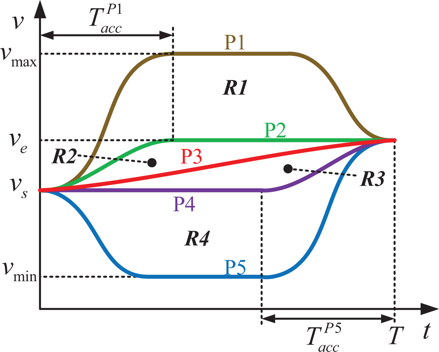
P4 profile consists of the CV and ACC phases and $T_{acc}^{P 4} = T_{acc}^{P 5}$ where $T_{acc}^{P 4}$ and $T_{acc}^{P 5}$ are the ACC time of P4 and P5.

Figure 3.

Five special profiles and four regions.

With these five profiles, $[S_{min}, S_{max}]$ is divided into four regions. In each region, the rules of phase components, orders, and time are stipulated in Table 1. Based on these rules, the velocity profiles in each region, such as the example profiles PR1–PR4 shown in Figure 4, have fixed forms, which guarantees that the solution of velocity planning is unique and reduces the computational load significantly. The corresponding velocity planning method will be described in the third section.

Table 1.

Rules of phase components, orders, and time of each phase in each region.

Region	Order of each phase	Rules of time	Features	Example profile
R1	ACC-CV-DEC	$T_{acc} = T_{acc}^{P1}$ $T_{cv} = T_{cv}^{P1}$ $T_{dec} = T_{dec}^{P1}$	S increases with $v_{max}^{act}$	PR1
R2	ACC-CV	—	S increases with $T_{c v}$	PR2
R3	CV-ACC	—	S increases with $T_{acc}$	PR3
R4	DEC-CV-ACC	$T_{dec} = T_{dec}^{P 5}$ $T_{cv} = T_{cv}^{P 5}$ $T_{acc} = T_{acc}^{P 5}$	S increases with $v_{min}^{act}$	PR4

Figure 4.

Example profile in each region.

Velocity planning method for PVT control based on the modified S-shaped ACC/DEC algorithm

Based on the modified S-shaped ACC/DEC algorithm, the velocity planning method is proposed to realize the PVT control. For the situations where the given conditions cannot be satisfied under the kinematic constraints, the corresponding processing procedures are also given. Based on Figure 4, the flowchart of velocity planning is depicted in Figure 5 and described in detail with eight steps as follows where assuming $0 \leq v_{s} \leq v_{e} \leq F$ :

Figure 5.

Velocity planning method based on the modified S-shaped ACC/DEC algorithm.

(1) Step 1: judging the rationality of the given conditions preliminarily.

The given time T might be insufficient to accelerate v_s to v_e . Hence, the maximum reachable end velocity $v_{e}^{max}$ under v_s , T, and $Φ_{k c}$ should be calculated as follows

\begin{array}{l} if T \leq \frac{2 a_{max}}{J_{max}} \\ then v_{e}^{max} = min (v_{s} + \frac{J_{max} T^{2}}{4}, F) \\ else v_{e}^{max} = min (v_{s} + a_{max} T - \frac{a_{max}^{2}}{J_{max}}, F) \end{array}

After that, the following judgment should be performed:

if $v_{e} \leq v_{e}^{max}$ , it means that v_e can be reached. Then, go to step 2.

if $v_{e} > v_{e}^{max}$ , it means T is too short and v_e is unreachable. Then, go to step 5.

(2) Step 2: calculating the maximum velocity $v_{max}$ in P1 profile and the minimum $v_{min}$ in P5 profile shown in Figure 4 as well as the corresponding displacement $S_{max}$ and $S_{min}$ .

The calculation procedures of $v_{max}$ and $v_{min}$ are shown in Appendix 1. Meanwhile, each phase time can be calculated. Then, $S_{max}$ and $S_{min}$ can be obtained as follows

S_{max} = \frac{v_{s} + v_{max}}{2} T_{acc}^{P 1} + v_{max} T_{c v}^{P 1} + \frac{v_{e} + v_{max}}{2} T_{dec}^{P 1}

S_{min} = \frac{v_{s} + v_{min}}{2} T_{dec}^{P 5} + v_{min} T_{cv}^{P 5} + \frac{v_{e} + v_{min}}{2} T_{acc}^{P 5}

Then, judge the relation between the given S and $[S_{min}, S_{max}]$ :

if $S \in [S_{min}, S_{max}]$ , it means the velocity can be planned under $Φ_{mc}$ and S. Then, go to Step 3.

if $S > S_{max}$ , it means S is too long for the given $Φ_{mc}$ . There are two sub-cases which can be chosen according to the user needs. If the condition of end velocity has higher priority than displacement, then got to step 6. Else, go to step 7.

if $S < S_{min}$ , it means S is too short. Similarly, two sub-cases exist. If the condition of end velocity is more important than displacement, then got to step 6. Else, go to step 8.

(3) Step 3: calculating the displacements S ₂, S ₃, and S ₄ of P2, P3, and P4 profiles shown in Figure 4.

Based on the specified rules given in subsection “The modified S -shaped ACC/DEC profile for PVT control,” S ₂, S ₃, and S ₄ can be calculated as follows

S_{2} = \frac{v_{s} + v_{e}}{2} T_{acc}^{P 1} + v_{e} (T - T_{acc}^{P 1})

S_{3} = \frac{v_{s} + v_{e}}{2} T

S_{4} = \frac{v_{s} + v_{e}}{2} T_{acc}^{P 5} + v_{s} (T - T_{acc}^{P 5})

Then, go to step 4.

(4) Step 4: velocity planning in different regions.

If $S \in [S_{min}, S_{4})$ , go to sub-step 4.1;

if $S \in [S_{4}, S_{3})$ , go to sub-step 4.2;

if $S \in [S_{3}, S_{2})$ , go to sub-step 4.3;

if $S \in [S_{2}, S_{max}]$ , go to sub-step 4.4.

Sub-step 4.1: velocity planning in region R4

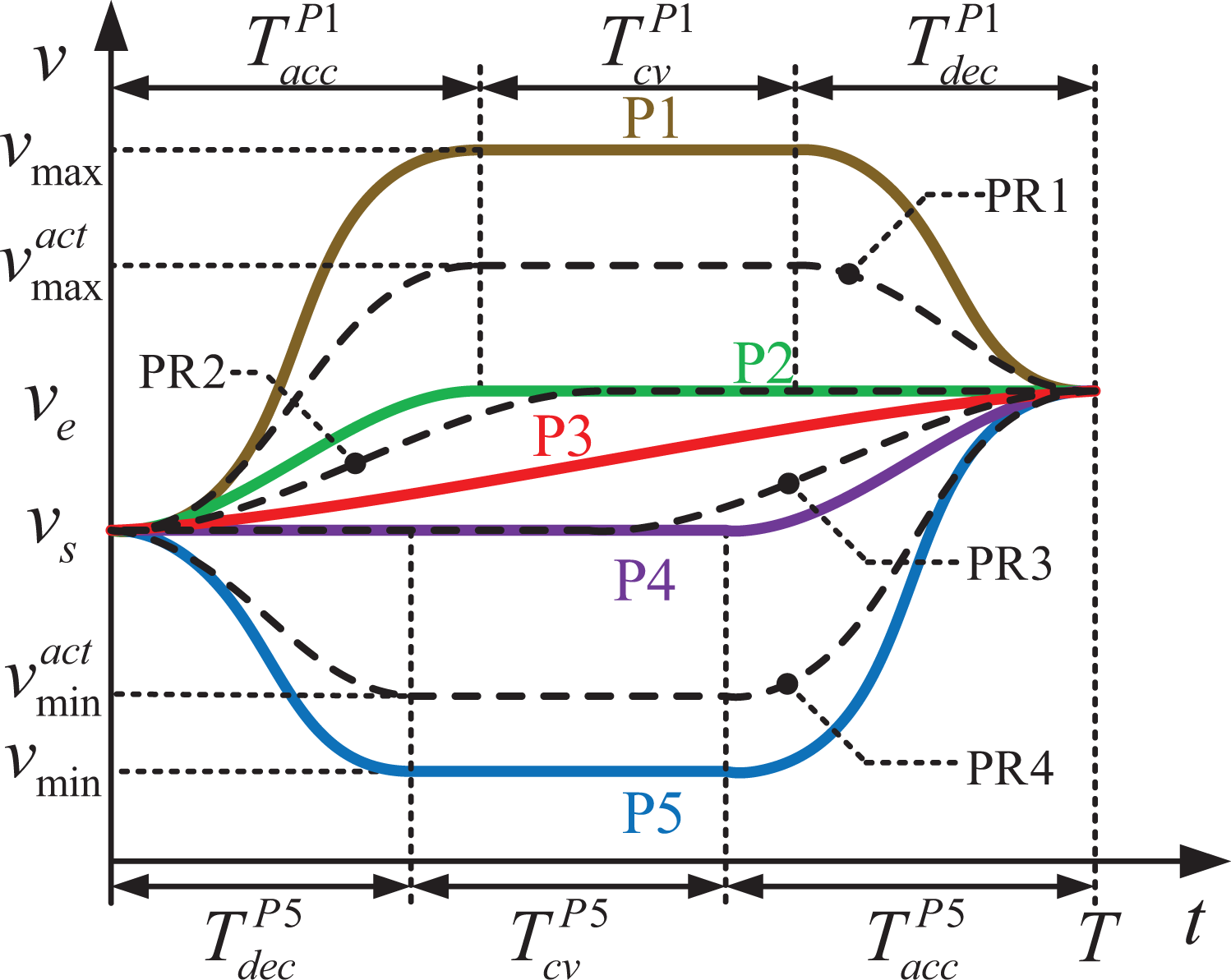
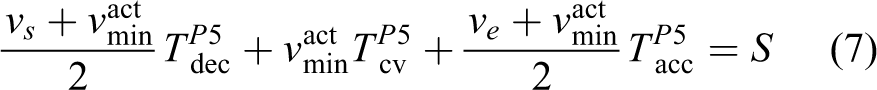
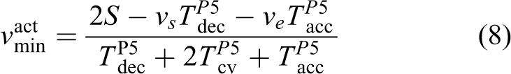
As the PR4 profile in Figure 6, the DEC, CV, and ACC phases all exist and the corresponding time is $T_{dec}^{P 5}$ , $T_{cv}^{P 5}$ , and $T_{acc}^{P 5}$ , respectively. The actual minimum velocity $v_{min}^{act}$ is selected as the variable and the following displacement equation can be constructed

\frac{v_{s} + v_{min}^{act}}{2} T_{dec}^{P 5} + v_{min}^{act} T_{cv}^{P 5} + \frac{v_{e} + v_{min}^{act}}{2} T_{acc}^{P 5} = S

Figure 6.

Actual jerk and duration of each section in region R4.

$v_{min}^{act}$ can be solved as

v_{min}^{act} = \frac{2 S - v_{s} T_{dec}^{P 5} - v_{e} T_{acc}^{P 5}}{T_{dec}^{P5} + 2 T_{cv}^{P 5} + T_{acc}^{P 5}}

As shown in Figure 6, the actual jerk and duration of each section in DEC phase can be calculated based on $v_{min}^{act}$ as follows

\begin{array}{l} if \frac{4 (v_{s} - v_{min}^{act})}{{(T_{d e c}^{P 5})}^{2}} < min (J_{max}, \frac{2 a_{max}}{T_{dec}^{P 5}}) \\ then T_{dec 1} = T_{dec 3} = \frac{T_{dec}^{P 5}}{2} \\ T_{dec 2} = 0 \\ else T_{dec 2} = \frac{2 (v_{s} - v_{min}^{act})}{a ਀ max} - T_{dec}^{P 5} \\ T_{dec 1} = T_{dec 3} = \frac{T_{dec}^{P5} - T_{dec 2}}{2} \\ J_{dec 3} = - J_{dec 1} = \frac{a_{max}}{T_{dec 1}} \end{array}

The jerk and duration of each section in ACC phase can also be calculated by equation (9) similarly. Therefore, the velocity planning is finished.

Sub-step 4.2: Velocity planning in region R3

As the PR3 profile in Figure 4, only the CV and ACC phases exist. The time of CV phase $T_{c v}$ is selected as variable. And the displacement equation can be constructed as

v_{s} T_{c v} + \frac{v_{s} + v_{e}}{2} (T - T_{c v}) = S

Then, $T_{cv}$ , the time of ACC phase $T_{acc}$ and its corresponding displacement $S_{acc}$ can be solved as follows

T_{cv} = \frac{2 S - (v_{s} + v_{e}) T}{v_{s} - v_{e}}

T_{acc} = T - T_{cv}

S_{acc} = \frac{v_{s} + v_{e}}{2} T_{acc}

Finally, similar to Sub-step 4.1, the jerk and duration of each section in ACC phase can be calculated based on equation (9).

Sub-step 4.3: Velocity planning in region R2

As the PR2 profile in Figure 4, only the ACC and CV phases exist and the time of CV phase $T_{cv}$ is selected as the variable to construct the following displacement equation

\frac{v_{s} + v_{e}}{2} (T - T_{cv}) + v_{e} T_{cv} = S

$T_{cv}$ can be solved as

T_{cv} = \frac{2 S - (v_{s} + v_{e}) T}{v_{e} - v_{s}}

Then, the time of ACC phase and other critical parameters can be calculated by equations (12) and (9).

Sub-step 4.4: Velocity planning in region R1

As the PR1 profile in Figure 4, the ACC, CV, and DEC phase are all existing and the corresponding time equals to $T_{acc}^{P 1}$ , $T_{acc}^{P 1}$ , and $T_{dec}^{P 1}$ , respectively. The actual maximum velocity $v_{max}^{act}$ can be the variable. Hence, the displacement equation can be constructed as

\frac{v_{s} + v_{max}^{act}}{2} T_{acc}^{P 1} + v_{max}^{act} T_{cv}^{P 1} + \frac{v_{e} + v_{max}^{act}}{2} T_{dec}^{P 1} = S

Then, $v_{max}^{act}$ can be solve as follows

v_{max}^{act} = \frac{2 S - v_{s} T_{acc}^{P 1} - v_{e} T_{dec}^{P 1}}{T_{acc}^{P 1} + 2 T_{cv}^{P 1} + T_{dec}^{P 1}}

Similar to Sub-step 4.1, the time and jerk of each section in ACC and DEC phase can be calculated based on equation (9).

(5) Step 5: Adjusting v_e to satisfy the time condition

In this situation, the given time T is too short that v_s cannot be accelerated to v_e . And the conditions of PVT control cannot be both satisfied. Therefore, to match the command beat, the conditions of end velocity and displacement should be abandoned. The end velocity v_e should be replaced by $v_{e}^{max}$ calculated in step 1. And the corresponding displacement S should be updated as

S = \frac{v_{s} + v_{e}^{max}}{2} T

Then, the jerk and time of each section can be obtained with the same procedures in step 4.

(6) Step 6: Abandoning the displacement condition

When coming to this step, it means the displacement condition cannot be satisfied with $Φ_{mc}$ . Meanwhile, v_e should be guaranteed. Therefore, the displacement condition should be abandoned. If $S < S_{min}$ ,Sshould be updated to $S_{min}$ . On the contrary, S should be replaced by $S_{max}$ when $S > S_{max}$ . Then, the jerk and time of each section in ACC and DEC phase can be calculated similar to sub-step 4.1 or 4.4.

(7) Step 7: Increasing the end velocity

Based on the maximum reachable end velocity $v_{e}^{max}$ obtained in step 1, the corresponding ACC time $T_{acc}^{v_{e}^{max}}$ and displacement $S_{਀}^{v_{e}^{max}}$ , which is the maximum reachable displacement under v_s , T, and $Φ_{kc}$ and consists of ACC and CV phases, can be calculated as follows

\begin{array}{l} if \frac{a_{max}^{2}}{J_{max}} + v_{s} \leq v_{e}^{max} \\ then T_{acc}^{v_{e}^{max}} = 2 \sqrt{\frac{v_{e}^{max} - v_{s}}{J_{max}}} \\ else T_{acc}^{v_{e}^{max}} = \frac{v_{e}^{max} - v_{s}}{a_{max}} + \frac{a_{max}}{J_{max}} \end{array}

S_{਀}^{v_{e}^{max}} = \frac{v_{s} + v_{e}^{max}}{2} T_{acc}^{max} + v_{e}^{max} (T - T_{acc}^{max})

Then,

if $S_{਀}^{v_{e}^{max}} \leq S$ , it means that the displacement conditions cannot be satisfied by increasing the end velocity. Hence, S and v_e should be replaced by $v_{e}^{max}$ and $S_{਀}^{v_{e}^{max}}$ .

else, $v_{e}^{max}$ should be reduced to $v_{e}^{max} ਀^{'}$ . $v_{e}^{max} ਀^{'}$ can be calculated as follows where the time of ACC phase is maintained as $T_{acc}^{v_{e}^{max}}$ and the rest is CV phase

v_{e}^{max} ਀^{'} = \frac{2 S - v_{s} T_{acc}^{v_{e}^{max}}}{2 T - T_{acc}^{v_{e}^{max}}}

Then, the time and jerk of each section in ACC phase can be calculated similar to sub-step 4.3.

8. Step 8: Reducing the end velocity

With the conditions of v_s , T, and $Φ_{kc}$ , the minimum reachable end velocity $v_{e}^{min}$ can be calculated as follows

\begin{array}{l} if T \leq \frac{2 a_{max}}{J_{max}} \\ then v_{e}^{min} = max (v_{s} - \frac{J_{max} T^{2}}{4}, 0) \\ else v_{e}^{min} = max (v_{s} - a_{max} T + \frac{a_{max}^{2}}{J_{max}}, 0) \end{array}

Based on $v_{e}^{min}$ , the corresponding DEC time $T_{dec}^{v_{e}^{min}}$ and displacement $S_{਀}^{v_{e}^{min}}$ , which is the minimum reachable displacement and consists of DEC phase, can be obtained as follows

\begin{array}{l} if \frac{a_{max}^{2}}{J_{max}} + v_{e}^{min} \leq v_{s} \\ then T_{dec}^{v_{e}^{min}} = 2 \sqrt{\frac{v_{s} - v_{e}^{min}}{J_{max}}} \\ else T_{dec}^{v_{e}^{min}} = \frac{v_{s} - v_{e}^{min}}{a_{max}} + \frac{a_{max}}{J_{max}} \end{array}

S_{਀}^{v_{e}^{min}} = \frac{v_{s} + v_{e}^{min}}{2} T_{dec}^{v_{e}^{min}} + v_{e}^{min} (T - T_{dec}^{v_{e}^{min}})

If $S \leq S_{਀}^{v_{e}^{min}}$ , it means that the displacement condition cannot be satisfied by reducing the end velocity. Therefore, S and v_e should be replaced by $S_{਀}^{v_{e}^{min}}$ and $v_{e}^{min}$ .

If $S > S_{਀}^{v_{e}^{min}}$ , $v_{e}^{min}$ should be increased to $v_{e}^{min} ਀^{'}$ . Similar to step 7, $v_{e}^{min} ਀^{'}$ can be calculated as follows where the time of DEC phase is maintained as $T_{dec}^{v_{e}^{min}}$ and the rest is CV phase

v_{e}^{min} ਀^{'} = \frac{2 S - v_{s} T_{dec}^{v_{e}^{min}}}{2 T - T_{dec}^{v_{e}^{min}}}

Then, the time and jerk of each section in DEC phase can be calculated and the velocity planning is finished.

For steps 5–8, the PVT conditions cannot be both satisfied. When coming to the next command period, the target displacement $S^{next}$ should be recalculated according to the implementation of current period while the corresponding start velocity $v_{s}^{next}$ is the end velocity of current period. And during the following motion, the tracking of end velocity and displacement can be conducted gradually, which is suitable for the real application. In particular, when there is no subsequent PVT command and the target end velocity or displacement is not reached, the velocity will be planned by the typical S-shaped ACC/DEC algorithm without considering the time condition.

Implementation and experimental results

In this section, the experiments are performed to evaluate the good performance of the proposed velocity planning method. Analysis and comparisons are also performed with some other representative methods such as the cubic and quintic polynomial interpolation algorithms.

Experimental setup

The experiments are conducted on a two-axis motion platform with Panasonic MBDH series servo derives and MHMD series motors. The layout of the experimental system is shown in Figure 7. The host computer generates PVT commands and sends them to the self-developed PC-based motion controller¹⁰ through Ethernet where the command period is 50 ms. The PVT commands come from a tracking system guided by machine vision. The tracking target including PVT conditions is given by machine vision and the mechanical system completes tracking. The configurations of the motion controller are shown in Table 2. Meanwhile, the axis control data can be sent to the corresponding servo derives by EtherCAT and the interpolation period is set to 1 ms. In addition, kinematic constraint parameters are shown in Table 3. The two axes’ PVT commands are shown in Figure 8(a) to (d).

Figure 7.

Layout of the experimental system.

Table 2.

Configurations of the motion controller.

Operating system	Windows 7 with KRTS
CPU	Intel(R) Core(TM) i5-4460, 3.2GHz
Memory	4.00 GB

Table 3.

Kinematic constraint parameters.

Parameters	X axis	Y axis
Maximum velocity F	400 mm/s	400 mm/s
Maximum acceleration $a_{max}$	1000 mm/s²	1000 mm/s²
Maximum jerk $J_{max}$	10000 mm/s³	10000 mm/s³

Figure 8.

PVT commands of the two axes.

Experiment results and comparisons

The target of velocity planning for PVT control is to satisfy the position, velocity, and time conditions under the kinematic constraints. Therefore, we judge the performance of velocity planning methods through comparing whether the motion parameters can be restricted in their allowable regions while complete the PVT motion.

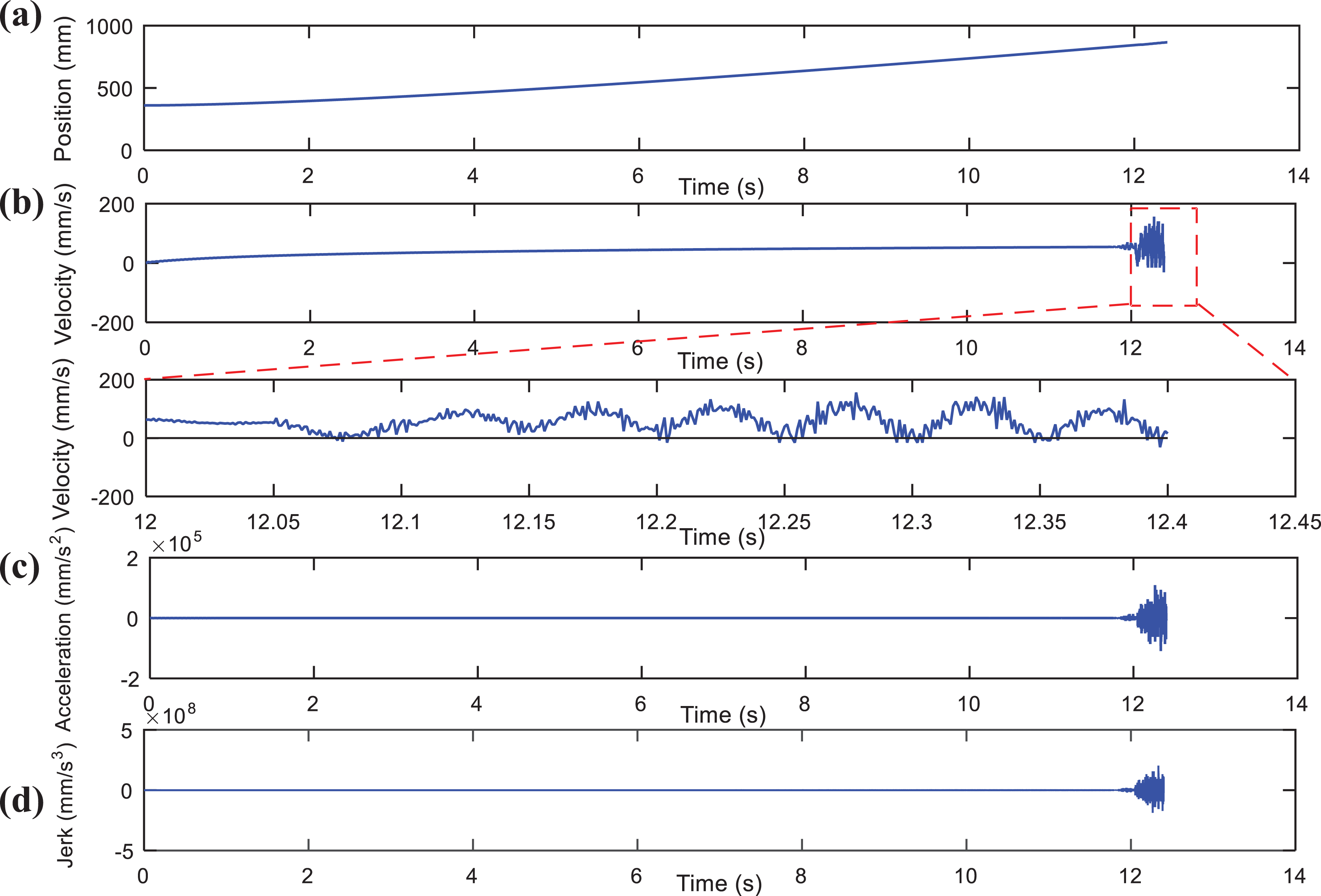
According to the PVT command sequences, the experiment results of the proposed velocity planning method are shown in Figures 9 and 10. As can be seen, smooth velocity and continuous acceleration profiles can be generated while all the motion parameters are restricted in their given ranges. For the commands which cannot be satisfied under the kinematic constraints, the given conditions are adjusted to match the constraints where the end velocity is set to a higher priority. In the last part, the given end velocity and position are not reached but there is no subsequent PVT command. Hence, the two axes are moved to the target position and end velocity directly based on the typical S-shaped ACC/DEC algorithm without considering the time condition.

Figure 9.

Experiment results of X axis by the proposed velocity planning method. (a) Position; (b) velocity; (c) acceleration; (d) jerk.

Figure 10.

Experiment results of Y axis by the proposed velocity planning method. (a) Position; (b) velocity; (c) acceleration; (d) jerk.

The experiment results obtained by the cubic and quintic polynomial interpolation methods are shown in Figures 11 and 12 and Figures 13 and 14, respectively. As shown in Figure 11(c) and 12(c), the acceleration profile obtained by the cubic polynomial method is discontinuous, which causes serious vibration and shock. Meanwhile, as can be seen form Figure 13(b) and 14(b), the velocity profile obtained by the quintic polynomial method has serious oscillations. Even in some interpolation periods, the velocity appears negative. In addition, the velocity, acceleration, and jerk obtained by the cubic and quintic polynomial methods are uncontrollable and exceed the kinematic constraints, which affects the motion smoothness and might cause damage to the drive and transmission components.

Figure 11.

Experiment results of X axis by the cubic polynomial method. (a) Position; (b) velocity; (c) acceleration; (d) jerk.

Figure 12.

Experiment results of Y axis by the cubic polynomial method. (a) Position; (b) velocity; (c) acceleration; (d) jerk.

Figure 13.

Experiment results of X axis by the quintic polynomial method. (a) Position; (b) velocity; (c) acceleration; (d) jerk.

Figure 14.

Experiment results of Y axis by the quintic polynomial method. (a) Position; (b) velocity; (c) acceleration; (d) jerk.

The real-time performance of the proposed velocity planning method is also tested during the experiments. The average and maximum computational time in each interpolation period are 1.562 μs and 10.523 μs, respectively, and much smaller than 1 ms. Therefore, the proposed method can always satisfy the real-time requirement with 1 ms interpolation period.

Conclusion and future works

In this article, a novel velocity planning method based on a modified S-shaped ACC/DEC algorithm is proposed for PVT control. For reasonable PVT commands, the given PVT conditions can be satisfied by this method with smooth velocity profile while the kinematic parameters can be limited in their allowable ranges. For unreasonable PVT commands, a series planning strategies are designed to adjust the given conditions according to the user needs, which is suitable for the real application. The comparative experiments have been conducted and validate the good performance and applicability of the proposed method.

For some devices, such as the serial industrial robots, their kinematic constraints are not fixed and vary with their position and posture. The proposed velocity planning method is only suitable for fixed constraints. Future work will focus on considering the variation characteristics of kinematic constraints during velocity planning to make full use of the motion performance of device. Therefore, the kinematic and dynamic models of devices need to be established to get accurate kinematic constraints.

Footnotes

Appendix 1: Calculation of v max and v min

Assuming $0 \leq v_{s} \leq v_{e} \leq F$ , the calculation of $v_{max}$ can be conducted with no more than three steps and its flowchart is shown in Figure 1A where $v_{max}^{(i)}$ is the assumed maximum velocity in Step Ai.

Based on the assuming of $v_{max}^{(1)}$ , the corresponding ACC time $T_{acc}^{(1)}$ can be calculated as follows

$\begin{array}{l} if v_{max}^{(1)} - v_{s} \leq \frac{a_{max}^{2}}{J_{max}} \\ then T_{acc}^{(1)} = 2 \sqrt{\frac{F - v_{s}}{J_{max}}} \\ else T_{acc}^{(1)} = \frac{F - v_{s}}{a_{max}} + \frac{a_{max}}{J_{max}} \end{array}$ (A1)

The DEC time $T_{dec}^{(1)}$ can also be calculated based on equation (A1). Then, the following judgments can be performed

if $T_{acc}^{(1)} + T_{dec}^{(1)} \leq T$ , then $v_{max} = F$

else, it means that $v_{max}$ should be smaller than F. Then, go to Step A2. Figure 1A.

The flowchart of the calculation of $v_{max}$ .

(2) Step A2: assuming $v_{max}^{(2)} = v_{e} + \frac{a_{max}^{2}}{J_{max}}$

Similar to Step A1, the ACC and DEC time $T_{acc}^{(2)}$ and $T_{dec}^{(2)}$ corresponding to $v_{max}^{(2)}$ can be calculated. The judgments are as follows:

if $v_{max}^{(2)} > F$ or $T_{acc}^{(2)} + T_{dec}^{(2)} > T$ , it means that $v_{max}$ should also be smaller than $v_{max}^{(2)}$ . Then, go to Step A3;

else if $T_{acc}^{(2)} + T_{dec}^{(2)} = T$ , then $v_{max} = v_{max}^{(2)}$

else, it can be inferred that $v_{max} \in (v_{max}^{(2)}, F)$ . Then, the dichotomy method can be employed to determine $v_{max}$ in $(v_{max}^{(2)}, F)$ .

(3) Step A3: assuming $v_{max}^{(3)} = v_{s} + \frac{a_{max}^{2}}{J_{max}}$

Based on equation (A1), the ACC and DEC time $T_{acc}^{(3)}$ and $T_{dec}^{(3)}$ corresponding to $v_{max}^{(3)}$ can be obtained. The similar judgments are as follows

If $v_{max}^{(3)} > F$ or $T_{acc}^{(3)} + T_{dec}^{(3)} > T$ , it means that $v_{max} \in [v_{e}, min (v_{max}^{3}, F))$ . Similar to Step A2, the dichotomy method can be used to calculate $v_{max}$ in $[v_{e}, min (v_{max}^{3}, F))$ ;

else if $T_{acc}^{(3)} + T_{dec}^{(3)} = T$ , then $v_{max} = v_{max}^{(3)}$

else, it can be concluded that $v_{max} \in (v_{max}^{(3)}, v_{max}^{(2)})$ . The dichotomy method can also be employed to calculate $v_{max}$ in $(v_{max}^{(3)}, v_{max}^{(2)})$ .

The calculation procedures of $v_{min}$ is similar to $v_{max}$ and its flowchart is shown inFigure 1B where $v_{min}^{(i)}$ is the assumed minimum velocity in Step Bi, $T_{acc}^{(i)} ਀^{'}$ and $T_{dec}^{(i)} ਀^{'}$ are the corresponding ACC and DEC time, respectively. Figure 1B.

The flowchart of the calculation of $v_{min}$ .

Acknowledgment

The authors would like to thank the supports from Natural Science Foundation of Shandong Province, Major Scientific and Technological Innovation Project of Shandong Province, and Major Projects of New and Old Kinetic Energy Conversion in Shandong Province.

Declaration of conflicting interests

The author(s) declared no potential conflicts of interest with respect to the research, authorship, and/or publication of this article.

Funding

The author(s) disclosed receipt of the following financial support for the research, authorship, and/or publication of this article: This study was supported by Natural Science Foundation of Shandong Province (Grant No. ZR2019QEE042), Major Scientific and Technological Innovation Project of Shandong Province (Grant Nos. 2019JZZY020121 and 2019JZZY010455), and Major Projects of New and Old Kinetic Energy Conversion in Shandong Province.

ORCID iDs

Shuai Ji

Chengrui Zhang

References

Cui

Mao

, et al. Spiral trajectory planning approach for underground cavity measurements based on laser scanning. Measurement. 2017; 110: 166–175.

Yue

Chen

, et al. Spline-interpolation based PVT algorithm and application in a bionic cockroach robot. 2010 11th international conference on control automation robotics & vision, Singapore, 7–10 December, 2010; 1742–1747.

Zhong

Luo

Chang

, et al. A real-time interpolator for parametric curves. Int J Machi Tools Manuf 2018; 125: 133–145.

Shi

Lin

. Joint motion planning of industrial robot based on modified cubic hermite interpolation with velocity constraint. Appl Sci-Basel 2021: 11(19): 1–21.

Liu

Yuan

. high accurate interpolation of NURBS tool path for CNC machine tools. Chin J Mech Eng 2016; 29: 1–10.

Kuo

Lin

. Dual-optimization trajectory planning based on parametric curves for a robot manipulator. Int J Adv Robot Syst 2020; 17(3): 1–14.

Ding

. Minimum-jerk trajectory planning pertaining to a translational 3-degree-of-freedom parallel manipulator through piecewise quintic polynomials interpolation. Adv Mech Eng 2020; 12(3): 1–18.

Ertl

. Computer graphics—Principles and practice. Berlin: Springer Vienna, 1996; 411–421.

Sang

Yao

, et al. An improved feedrate scheduling method for NURBS interpolation in five-axis machining. Precis Eng 2020; 64: 70–90.

10.

Zhang

, et al. An optimized feedrate scheduling method for CNC machining with round-off error compensation. Int J Adv Manuf Technol 2018; 97: 2369–2381.

11.

Wang

Zhang

Dong

, et al. NURBS Interpolator with adaptive smooth feedrate scheduling and minimal feedrate fluctuation. Int J Precis Eng Manuf 2019; 21(2), 273–290.

12.

Wang

Lin

Chang

, et al. Velocity planning for astronaut virtual training robot with high-order dynamic constraints. Robotica. 2020; 38(12): 2121–2137.

13.

Sun

Wang

Liu

, et al. Enhanced feedrate scheduling algorithm for CNC system with acceleration look-ahead and sin(2) acceleration profile. Int J Adv Manuf Technol 2021; 1–15.

14.

Huang

Zhu

. Feedrate scheduling for interpolation of parametric tool path using the sine series representation of jerk profile. Proceed Institut Mech Eng-Part B: J Eng Manuf 2016; 231(13): 2359–2371.

15.

Yuan

, et al. Feedrate Scheduling of NURBS interpolation based on a novel Jerk-continuous ACC/DEC algorithm. IEEE Access 2018; 6: 66403–66417.

16.

Chen

Dong

Ding

. An efficient method for collision-free and jerk-constrained trajectory generation with sparse desired way-points for a flying robot. Sci China Technol Sci 2021; 64(8): 1719–1731.

17.

Weng

Kuo

CFJ

. Jerk decision for free-form surface effects in multi-axis synchronization manufacturing. Int J Adv Manuf Technol 2019; 105(1-4): 799–812.

18.

Fang

Liu

, et al. Smooth and time-optimal S-curve trajectory planning for automated robots and machines. Mech Mach Theory 2019; 137: 127–153.

19.

Zhang

, et al. An optimal curvature-smooth transition algorithm with axis jerk limitations along linear segments. Int J Adv Manuf Technol 2018; 95: 875–888.

20.

Liu

Fang

, et al. A feedrate optimization method for CNC machining based on chord error revaluation and contour error reduction. Int J Adv Manuf Technol 2020; 111(11-12): 3437–3452.

21.

Zhang

Chen

, et al. A novel time-rounding-up-based feedrate scheduling method based on S-shaped ACC/DEC algorithm. Int J Adv Manuf Technol 2019; 104(5-8):2073–2088.

22.

Chen

Yang

ECY

. Near time-optimal S-curve velocity planning for multiple line segments under axis constraints. IEEE Trans Ind Electr 2018; 65(12): 9582–9592.

23.

Yang

Zhang

H-T

Ding

. Contouring error control of the tool center point function for five-axis machine tools based on model predictive control. Int J Adv Manuf Technol 2017; 88: 2909–2919.

24.

Wang

Luo

. A planning method for multi-axis point-to-point synchronization based on time constraints. IEEE ACCESS. 2020; 8: 85575–85604.

Velocity planning method for position–velocity–time control based on a modified S-shaped acceleration/deceleration algorithm

Abstract

Keywords

Introduction

Typical S-shaped ACC/DEC profile and its modification for PVT control

The typical S-shaped ACC/DEC profile

The modified S-shaped ACC/DEC profile for PVT control

Velocity planning method for PVT control based on the modified S-shaped ACC/DEC algorithm

Implementation and experimental results

Experimental setup

Experiment results and comparisons

Conclusion and future works

Footnotes

Appendix 1: Calculation of v max and v min

Acknowledgment

Declaration of conflicting interests

Funding

ORCID iDs

References